Turbulent lithosphere deformation in the Tibetan Plateau
Xing Jian, Wei Zhang, Qiang Deng, Yongxiang Huang

TL;DR
This paper reveals turbulence-like statistical features in the deformation of the Tibetan Plateau, showing dual cascade behaviors and universal scaling properties, which challenge existing geodynamic models and suggest a geostrophic turbulence interpretation.
Contribution
It uncovers turbulence-like statistics and dual cascade behaviors in Tibetan Plateau deformation, providing new insights and challenges for geodynamic modeling.
Findings
Evidence of turbulence-like statistics in plateau deformation
Dual-power-law behavior indicating two cascade regimes
Similarity of structure-function exponents with atmospheric turbulence
Abstract
In this work, we show that the Tibetan Plateau deformation demonstrates a turbulence-like statistics, e.g., spatial invariance cross continuous scales. A dual-power-law behavior is evident to show the existence of two possible conversation laws for the enstrophy-like cascade on the range and kinetic-energy-like cascade on the range . The measured second-order structure-function scaling exponents are similar with the counterpart of the Fourier scaling exponents observed in the atmosphere, where in the latter case the earth rotation is relevant. The turbulent statistics observed here for nearly zero Reynolds number flow is favor to be interpreted by the geostrophic turbulence theory. Moreover, the intermittency correction is recognized with an intensity to be close to the one of the hydrodynamic…
Click any figure to enlarge with its caption.
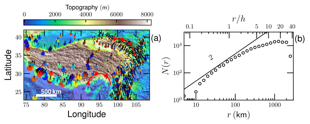 Figure 1
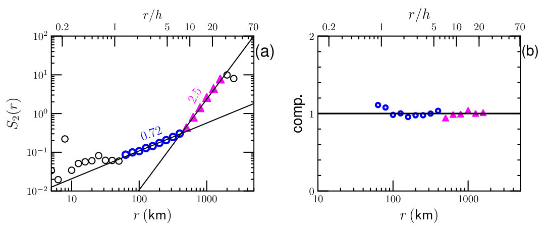 Figure 2
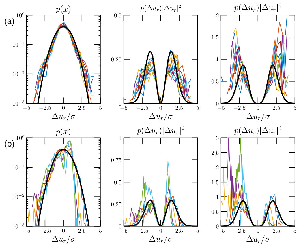 Figure 3
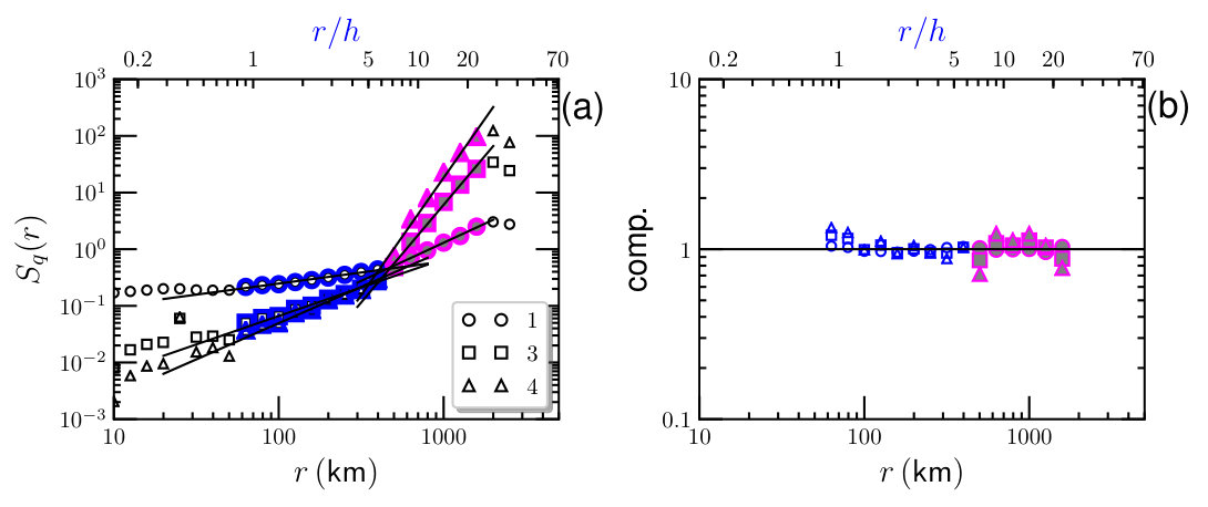 Figure 4
 Figure 5
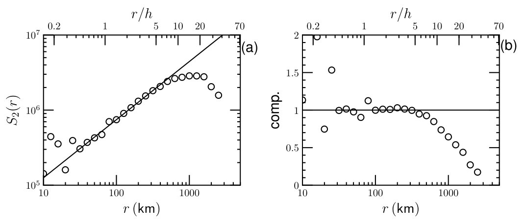 Figure 6
Peer Reviews
No public reviews on file for this paper yet. If you reviewed it on a platform where reviews are public (OpenReview, ICLR, NeurIPS, ICML), you can paste yours below so the community can read it here.
Videos
No videos yet. Explain this paper in a talk, walkthrough, or lecture? Add one.
Turbulent lithosphere deformation in the Tibetan Plateau
Xing Jian ( )
State Key Laboratory of Marine Environmental Science, College of Ocean and Earth Sciences, Xiamen University, Xiamen 361102, China
Wei Zhang ( Ρ)
State Key Laboratory of Marine Environmental Science, College of Ocean and Earth Sciences, Xiamen University, Xiamen 361102, China
Qiang Deng ( ǿ)
State Key Laboratory of Marine Environmental Science, College of Ocean and Earth Sciences, Xiamen University, Xiamen 361102, China
Yongxiang Huang ( )
State Key Laboratory of Marine Environmental Science, College of Ocean and Earth Sciences, Xiamen University, Xiamen 361102, China
Abstract
In this work, we show that the Tibetan Plateau deformation demonstrates a turbulence-like statistics, e.g., spatial invariance cross continuous scales. A dual-power-law behavior is evident to show the existence of two possible conversation laws for the enstrophy-like cascade on the range \mathrm{k}\mathrm{m} and kinetic-energy-like cascade on the range $50\lesssim r\lesssim 500\,$\mathrm{k}\mathrm{m}. The measured second-order structure-function scaling exponents are similar with the counterpart of the Fourier scaling exponents observed in the atmosphere, where in the latter case the earth rotation is relevant. The turbulent statistics observed here for nearly zero Reynolds number flow is favor to be interpreted by the geostrophic turbulence theory. Moreover, the intermittency correction is recognized with an intensity to be close to the one of the hydrodynamic turbulence of high Reynolds number turbulent flows, implying a universal scaling feature of very different turbulent flows. Our results not only shed new light on the debate regarding the mechanism of the Tibetan Plateau deformation, but also lead to new challenge for the geodynamic modelling using Newton or non-Newtonian model that the observed turbulence-like features have to be taken into account.
pacs:
47.27.eb,94.05.Lk, 47.27.Gs
I Introduction
The Tibetan plateau, usually referred to as the “Roof of the World” expresses a double-thickened crust and stands at an average elevation of 5 over a region of approximately 3 million , see Fig. 1 (a). Given the India-Eurasia collision and uplift of the plateau as the most significant geological events on the earth during Cenozoic time, Tibetan plateau has been widely regarded as an ideal field laboratory for understanding the geodynamic processes of continental collision, deformation and the interactions between uplift and global climate change Harrison et al. (1992); Raymo and Ruddiman (1992); Molnar et al. (1993); An et al. (2001). However, how the Tibetan plateau deformed and grew remains highly controversial. Proposed hypotheses mainly include, 1) rigid plates or blocks northward propagating subduction and extrusion Tapponnier et al. (1982, 2001), 2) convective removal of mantle lithosphere and rapid, continuous and entire deformation Molnar et al. (1993), and 3) lower crustal flow rather than substantial upper crustal thickening contributes the plateau deformation and uplift Royden et al. (1997); Clark and Royden (2000). These models are very creative and highly provocative, represent distinct driving mechanisms and kinematic descriptions of surface deformation, and thus have attracted considerable attention for decades. To test these hypotheses, a great number of geological and geophysical data and various methods have been used, primarily including paleoaltimetry, thermochronology, basin analysis and magnetostratigraphy, global positioning system (GPS) data and subsurface geophysical data analyses Zhang et al. (2004); Rowley and Currie (2006); Clark et al. (2010); Bai et al. (2010); Lease et al. (2012); Hoke et al. (2014); Jian et al. (2018). Although none of these models uniquely account for all of the geological and geophysical data and observations, more and more studies are aware of the presence of continuous medium and the important role of the rheology in the surface deformation of the Tibetan Plateau Clark and Royden (2000); Zhang et al. (2004); Royden et al. (2008). However, to the best of our knowledge, the spatial scale invariance of such flowing deformation has never been taken into account.
Turbulence or turbulence-like phenomena are ubiquitous in the nature, which is often characterized by scale invariance in both spatial and temporal domains. It ranges from the evolution of the universe (Gibson, 1996), movement of atmosphere and ocean (Nastrom et al., 1984; Thorpe, 2005), the painting by Leonardo da Vinci (Frisch, 1995) or van Gogh (Aragón et al., 2008), collective motion of bacteria (Wensink et al., 2012; Qiu et al., 2016), the Bose-Einstein condensate (Navon et al., 2016), financial activity (Ghashghaie et al., 1996; Schmitt et al., 1999; Lux, 2001; Li and Huang, 2014; Mandelbrot and Hudson, 2007), etc. Note that turbulence is usually recognized by its main features that a broad range of spatial and temporal scales or many degrees of freedom are excited in the dynamical system Groisman and Steinberg (2000); Alexakis and Biferale (2018). The turbulence theory is thus such theory to describe the energy injection and dissipation patterns or the balance among other physical quantities. This pattern could be quite different for different dynamical systems. For instance, in the classical three-dimensional hydrodynamical turbulence, the energy is injected into the system at large-scale and is transferred to small-scale, and so on, until to the viscosity scale where the kinetic energy is converting to heat Frisch (1995). This is a forward energy cascade with the famous Kolmogorov -law for the spatial Fourier power spectrum of high Reynolds number turbulent flows, e.g., . While in the two-dimensional turbulence, the energy (resp. enstrophy, square of vorticity) is inputted into the system through a middle scale. It is then transferred upward (resp. downward) due to energy (resp. enstrophy) conservation with a -law for large-scale part (resp. scaling law for small-scale part) Kraichnan (1967). Another famous example is the theory of geostrophic turbulence, in which the horizontal pressure gradient is balanced by the Coriolis force Charney (1971). A potential enstrophy cascade with a scaling exponent (resp. large-scale part) and energy cascade with a scaling exponent (small-scale part) are then presented Vallgren et al. (2011).
In this work, in the spirit of the turbulence theory, we show that the Tibetan Plateau deformation also demonstrates a turbulence-like statistics, e.g., spatial invariance cross continuous scales. A dual-power-law behavior is evident to show the existence of two possible conversation laws for the (potential) enstrophy-like cascade on the range \mathrm{k}\mathrm{m} and kinetic energy-like cascade on the range $50\lesssim r\lesssim 500\,$\mathrm{k}\mathrm{m}. The measured second-order structure-function (SF) scaling exponents are similar with the ones observed in the atmosphere Nastrom et al. (1984), where in the latter case the earth rotation is relevant. The turbulent statistics observed here is favor to be interpreted by the geostrophic turbulence theory, where a large-scale forcing due to the India-Euraisa collision might be balanced by the Coriolis force. Furthermore, the intermittency correction is identified with a strength close to the one of three-dimensional hydrodynamical turbulence of high Reynolds number turbulent flows. Our results not only shed new light on the debate regarding the mechanism of the Tibetan Plateau deformation, but also lead to new challenge for the geodynamic modeling that the observed turbulent features have to be taken into account.
II Data and Methodology
The GPS velocity data set is provided in Ref. Zhang et al. (2004). Figure 1 shows the deformation velocity unit vector collected from 553 monitoring locations Zhang et al. (2004), where the topology provided by ETOPO1 111https://www.ngdc.noaa.gov/mgg/global is illustrated in a color map. The symbols indicates the velocity magnitude in the range \mathrm{c}\mathrm{m}\mathrm{/}\mathrm{y}\mathrm{e}\mathrm{a}\mathrm{r}. Their mean magnitude and standard deviation respectively are $1.27\,$\mathrm{c}\mathrm{m}\mathrm{/}\mathrm{y}\mathrm{e}\mathrm{a}\mathrm{r} and \mathrm{c}\mathrm{m}\mathrm{/}\mathrm{y}\mathrm{e}\mathrm{a}\mathrm{r}. Figure [1](#S2.F1) (b) shows the distribution of the neighbor distance of two pair of monitoring locations. Note that a power-law behavior with a scaling exponent $2$ indicates a homogeneous distribution of these monitoring stations, which is illustrated by a solid line for reference in Fig. [1](#S2.F1) (b). Roughly speaking, the monitoring stations are homogeneous distributed on the scale range $20\lesssim r\lesssim 200\,$\mathrm{k}\mathrm{m} (resp., , where \mathrm{k}\mathrm{m}$$ is the average depth of the Tibetan lithosphere).
The velocity pattern demonstrates an anticyclone (clockwise) structure, showing eddy-like motions. To characterize the motions more quantitatively, we introduce here a second-order moment of the structure-function (SF), which is written as,
[TABLE]
where is the great circle distance, is the velocity vector. For a scaling process, one expects the following relation,
[TABLE]
Figure 2 (a) shows the measured second-order SF . A dual-power-law behavior is evident respectively on the range \mathrm{k}\mathrm{m} (resp., $0.7\lesssim r/h\lesssim 7$) and $500\lesssim r\lesssim 2,000\,$\mathrm{k}\mathrm{m} (resp. ). The experimental scaling exponent are found to be and , where the error indicates a fitting confidence level. According to the Wiener-Khinchin theorem, the Fourier power spectrum of the deformation velocity also follows a power-law behavior (Frisch, 1995; Huang et al., 2010),
[TABLE]
Thus the scaling exponent of the Fourier power spectrum indicated by second-order SF are and , which could be verified in the future when more data are available from either observation or numerical simulation.
III Results and Discussions
III.1 Scaling of deformation
The value of the scaling exponent provided by the second-order SF is close to , which implies a kinetic energy cascade that has been predicted by several theories. For example, the Kolmogorov 1941 theory for three-dimensional homogeneous and isotropic turbulence for the fully developed hydrodynamic turbulence Frisch (1995); the Kraichnan 1967 theory for the two-dimensional turbulence Kraichnan (1967); Charney 1971 theory for the geostrophic turbulence (Charney, 1971). The another scaling value may imply a (potential) enstrophy conservation in the framework of two-dimensional turbulence Kraichnan (1967) or geostrophic turbulence Charney (1971). As aforementioned, the mechanism behind the power-law is the pattern between injection and dissipation. Therefore, to exclude any possible explanations, the external force that driving the lithosphere deformation has to be recognized. A possible driving force is from the collision between the Indian and Eurasian plates with a large-scale instability above \mathrm{k}\mathrm{m}. Another possibility of the external force is at scale around $500\,$\mathrm{k}\mathrm{m}, where the kinetic energy is injected into the system via the thermal plumes of the mental convection Zhong and Zhang (2005). Due to the complexity of the current problem, such balance pattern is more complex than the ideal 2D turbulence theory or geostrophic turbulence theory. With the limited data, we cannot rule out any one of them. A scale-to-scale energy/enstrophy flux should be checked with attention to identify the cascade direction when the data is available Alexakis and Biferale (2018); Zhou et al. (2015).
It is interesting to note that a similar dual-power-law behavior has been reported for the atmospheric movement in the Fourier space with the same separation scale around \mathrm{k}\mathrm{m} around the same latitude Nastrom *et al.* ([1984](#bib.bib18)); Gao *et al.* ([2016](#bib.bib39)), where the separation scale $500\,$\mathrm{k}\mathrm{m} is determined by geostrophic balance that described by the Rossby number, see definition below. According to Vallgren et al. (2011), if the large-scale forcing due to the India-Eurasia collision is applicable, then the geostropic turbulence is favorable. Note that the power-law behavior observed here is consistent with the discovery of the continuous deformation by Zhang et al. (2004) for the spatial scale above \mathrm{k}\mathrm{m}$$.
The basic characteristic of turbulent system is intermittency, manifested as intense and sporadic fluctuations on different scale of motions. It is one of the most fascinating feature of the hydrodynamic turbulence Frisch (1995), which has been reported also for other complex dynamic systems Schmitt and Huang (2016). To track such intermittency correction, a high-order SFs is introduced, i.e.,
[TABLE]
where is the scaling exponents for high-order SFs. is linear with if there is no intermittency correction and vice versa. The deviation from linear relation is usually believed to be an effect of the nonlinear interactions between different scales (Frisch, 1995), manifesting as a large variation of the considered data (Schmitt and Huang, 2016). Note that the can be also defined via a dependent probability density function (pdf) of velocity difference ,
[TABLE]
where is the th-order integral kernel. To check whether the statistics is convergent or not, we plot the measured pdf and the corresponding integral kernel in Fig. 3 for (a) \mathrm{k}\mathrm{m} and (b) $500\lesssim r\lesssim 2000\,$\mathrm{k}\mathrm{m}. It suggests a safe estimation of the high-order SFs on the range with this limit data set.
High-order SFs are then calculated with . However, only the case for is discussed below. Figure 4 (a) shows the SFs for (), () and (), where the solid line is a least square fitting. The dual-power-law is evident on the same scale ranges. Figure 4 (b) shows the corresponding compensated curves to highlight the observed power-law behavior. Figure 5 (a) shows the measured scaling exponents for small-scale part () and large-scale one (). For comparison, for the energy cascade and for the (potential) enstrophy cascade are also shown. First of all, the experimental curves are convex, confirming the existence of intermittency correction. Secondly, the scaling exponent for the scale on the range \mathrm{k}\mathrm{m} is close to the value $\zeta(q)=q/3$, indicating an energy cascade with intermittency correction. Thirdly, the scaling exponent $\zeta^{\mathrm{L}}(q)$ for the scale on the range $500\lesssim r\lesssim 2,000\,$\mathrm{k}\mathrm{m} close to the value , indicating a (potential) enstrophy cascade with intermittency correction. To characterize the intensity of intermittency, the extended-self-similarity (Benzi et al., 1993) is resorted via plotting versus , see Fig. 5 (b). The experimental curves and collapse with each other when . While the former one is slightly above the latter one when . For comparison, the scaling value of the hydrodynamical turbulence (thick solid line) (Schmitt, 2006) and passive scalar turbulence (thin solid line) (Schmitt, 2005) are also illustrated. Graphically, the measured scaling exponents are close to the one of hydrodynamical turbulence of high Reynolds number turbulent flows, implying a possible universal feature of very different turbulent systems (Wang and Huang, 2017).
III.2 Scaling of topography
To cross verify the above observation, the topography of the Tibetan Plateau provided by ETOPO1 is analyzed below (Gagnon et al., 2003). The evolution of the elevation can be approximately written as,
[TABLE]
where is the initial elevation, and the typical vertical velocity can be treated as average vertical velocity since it is a very slowly variation with time. The elevation difference is thus an approximation of the velocity difference,
[TABLE]
where is assumed when is smaller than a certain value, e.g. \mathrm{k}\mathrm{m}. High-order SFs, e.g., $S_{q}(r)=\langle|\Delta_{r}h|^{q}\rangle$ are estimated. A single power-law behavior is observed on the scale range $50\lesssim r\lesssim 500\,$\mathrm{k}\mathrm{m} (resp. ) in Fig. 6 (a). The measured second-order SF scaling exponent is to be , which agrees well with the one of the horizontal deform velocity obtained on the same scale range. Figure 6 (b) shows the corresponding compensated curve to emphasize the observed scaling behavior. The measured high-order scaling exponent with is also shown in Fig. 5 as . Graphically, it agrees well with the one of the horizontal velocity, confirming the existence of the turbulence-like dynamics.
III.3 Several key parameters
Finally, several possible relevant parameters are discussed as following. A scale dependent Reynolds number can be defined as,
[TABLE]
where is the density, the velocity, the spatial scale and is the dynamic viscosity. It characterizes the ratio between the inertia and viscosity forces. Typical values in Tibet are \mathrm{g}\mathrm{/}\mathrm{c}\mathrm{m}^{3} (Li *et al.*, [2017](#bib.bib46)), $u\simeq 1.27\,$\mathrm{c}\mathrm{m}\mathrm{/}\mathrm{y}\mathrm{e}\mathrm{a}\mathrm{r} (Zhang et al., 2004), \mathrm{P}\mathrm{a}\cdot\mathrm{s} (Shi and Cao, [2008](#bib.bib47)), respectively. Considering the spatial scale $r$ from $50\,$\mathrm{k}\mathrm{m} to \mathrm{k}\mathrm{m}$$, one has a Reynold number on the range , suggesting that the viscosity force is more relevant than the inertial one in the current problem. Note that turbulence is usual associated with the high-Reynolds number flows, where the inertia of fluid is relevant and the viscosity force can be neglected (Frisch, 1995). Turbulence without inertia (Larson, 2000) have been reported for the bacterial turbulence (Wensink et al., 2012; Qiu et al., 2016; Wang and Huang, 2017), elastic turbulence (Groisman and Steinberg, 2000, 2001), etc., with nearly zero Reynolds number. As aforementioned, the balance pattern could be quite different from the classical hydrodynamic turbulence. However, they might share the universal turbulent features, such as the same strength of the intermittency (Wang and Huang, 2017).
Due to the earth rotation, the Coriolis force could be important. A scale-dependent Rossby number is introduced to characterize this effect, which is written as,
[TABLE]
where is the so-called Coriolis frequency, and \mathrm{r}\mathrm{a}\mathrm{d}\mathrm{/}\mathrm{s} the angular frequency of planetary rotation and $\phi\simeq 30\,$\mathrm{d}\mathrm{e}\mathrm{g}\mathrm{r}\mathrm{e}\mathrm{e} the latitude. It measures the ratio between the inertial force and Coriolis force. Taking the same typical velocity and length scales as for the Reynolds number, one has typical value of on the range , implying that the Coriolis force is more relevant than the inertial one.
Finally, a scale-dependent Deborah number is defined as,
[TABLE]
where refers to the stress relaxation time for a given spatial scale , and is the time scale of observation. It characterizes the ratio of the relaxation time characterizing the time it takes for a material to adjust to applied stresses or deformations, and the characteristic time scale of an experiment probing the response of the material. At lower Deborah numbers, the material behaves in a more fluid-like manner, with an associated Newtonian viscous flow. At higher Deborah numbers, the material behavior enters the non-Newtonian regime, increasingly dominated by elasticity and demonstrating solid-like behavior. Typical examples are flows of ice-river, asphaltum, etc., that for a long time observation and thus a small Deborah number, they behave in the fluid-like manner Reiner (1964). For the current case, the Deborah number is estimated on the range , suggesting that the lithosphere deformation can be treated as fluid flow.
IV Conclusion
In summary, in this work, the lithosphere deformation of the Tibetan Plateau is analyzed in the spirit of the multiscale statistics from turbulence community. The dual-power-law behavior is evident respectively on the range \mathrm{k}\mathrm{m} (resp. $0.7\lesssim r/h\lesssim 7$) and $500\lesssim r\lesssim 2,000\,$\mathrm{k}\mathrm{m} (resp. ). The scaling feature of the former scaling range indicates an energy cascade, while the one of the latter scaling range implies a (potential) enstrophy cascade, which might be interpreted in the framework of geostrophic turbulence since one possible external force can be identified from the India-Eurasia collision with a spatial scale above \mathrm{k}\mathrm{m}$$. The similar multiscale feature with the one from atmosphere suggests that they might share the similar dynamic, e.g., the balance between large-scale force and Coriolis force. However, to exclude any other possibility, a scale-to-scale energy/enstrophy flux has to be estimated either in Fourier space or physical domain to determine the cascade direction (Alexakis and Biferale, 2018; Zhou et al., 2015), see example in Ref. (Wang and Huang, 2017). Moreover, the intermittency is revealed via the high-order SFs. With the help of extended-self-similarity, the intensity of intermittency is found to be the same as the one of hydrodynamic turbulence of high Reynolds turbulent flows, showing a universal feature of very different turbulent flows, even for nearly zero Reynolds number flows (Groisman and Steinberg, 2000, 2001; Qiu et al., 2016; Wang and Huang, 2017). Our results not only shed new light on the understanding of the lithosphere deformation of Tibetan Plateau, but also lead to new challenge for the geophysical modelling using Newtonian or non-Newtonian fluid model that the observed turbulent features have to be taken into account.
Acknowledgements.
This work is sponsored by the National Natural Science Foundation of China (under Grant No. 11732010 and 41806052), and partially by the Fundamental Research Funds for the Central Universities (Grant No. 20720180120, 20720180123 and 20720170073) and MEL (State Key Laboratory of Marine Environmental Science) Internal Research Fund (Grant No. MELRI1802). We thank professor J. Q. Zhong and F. G. Schmitt for useful discussion. The source code and GPS data is available at: 222https://github.com/lanlankai. We thank the two anonymous reviewers for their careful reading and insightful comments and suggestions.
The reference list from the paper itself. Each links out to its DOI / PubMed record.
- 1Harrison et al. (1992) T. M. Harrison, P. Copeland, W. S. F Kidd, and A. Yin, “Raising Tibet,” Science 255 , 1663 (1992).
- 2Raymo and Ruddiman (1992) M. E Raymo and W. F. Ruddiman, “Tectonic forcing of late cenozoic climate,” Nature 359 , 117–122 (1992).
- 3Molnar et al. (1993) P. Molnar, P. England, and J. Martinod, “Mantle dynamics, uplift of the tibetan plateau, and the indian monsoon,” Rev. Geophys. 31 , 357–396 (1993).
- 4An et al. (2001) Z.S. An, J. E. Kutzbach, W. L. Prell, and S. C. Porter, “Evolution of Asian monsoons and phased uplift of the Himalaya–Tibetan plateau since Late Miocene times,” Nature 411 , 62–66 (2001).
- 5Tapponnier et al. (1982) P. Tapponnier, G. Peltzer, A. Y. Le Dain, R. Armijo, and P. Cobbold, “Propagating extrusion tectonics in Asia: New insights from simple experiments with plasticine,” Geology 10 , 611–616 (1982).
- 6Tapponnier et al. (2001) P. Tapponnier, Z. Q. Xu, F. Roger, B. Meyer, N. Arnaud, G. Wittlinger, and J. S. Yang, “Oblique stepwise rise and growth of the Tibet Plateau,” Science 294 , 1671–1677 (2001).
- 7Royden et al. (1997) L. H. Royden, B. C. Burchfiel, R. W. King, E. Wang, Z. L. Chen, F. Shen, and Y. P. Liu, “Surface deformation and lower crustal flow in eastern Tibet,” Science 276 , 788–790 (1997).
- 8Clark and Royden (2000) M. K. Clark and L. H. Royden, “Topographic ooze: Building the eastern margin of Tibet by lower crustal flow,” Geology 28 , 703–706 (2000).