AKLT models on decorated square lattices are gapped
Nicholas Pomata, Tzu-Chieh Wei

TL;DR
This paper proves that AKLT models on decorated square lattices are gapped for certain decorations, extends numerical methods to establish gaps on various lattices, and shows these states are not Ne9el ordered.
Contribution
The paper analytically proves the spectral gap for decorated square and hybrid lattices and introduces advanced numerical techniques to determine gaps on additional lattices.
Findings
AKLT models on decorated square lattices are gapped for na0a0 4
Numerical methods establish gaps for na0a0 2 on triangular and cubic lattices
Decorated cubic lattice AKLT states are not Ne9el ordered
Abstract
The nonzero spectral gap of the original two-dimensional Affleck-Kennedy-Lieb-Tasaki (AKLT) models has remained unproven for more than three decades. Recently, Abdul-Rahman et al. [arXiv:1901.09297] provided an elegant approach and proved analytically the existence of a nonzero spectral gap for the AKLT models on the decorated honeycomb lattice (for the number of spin-1 decorated sites on each original edge no less than 3). We perform calculations for the decorated square lattice and show that the corresponding AKLT models are gapped if . Combining both results, we also show that a family of decorated hybrid AKLT models, whose underlying lattice is of mixed vertex degrees 3 and 4, are also gapped for . We develop a numerical approach that extends beyond what was accessible previously. Our numerical results further improve the nonzero gap to , including the…
Click any figure to enlarge with its caption.
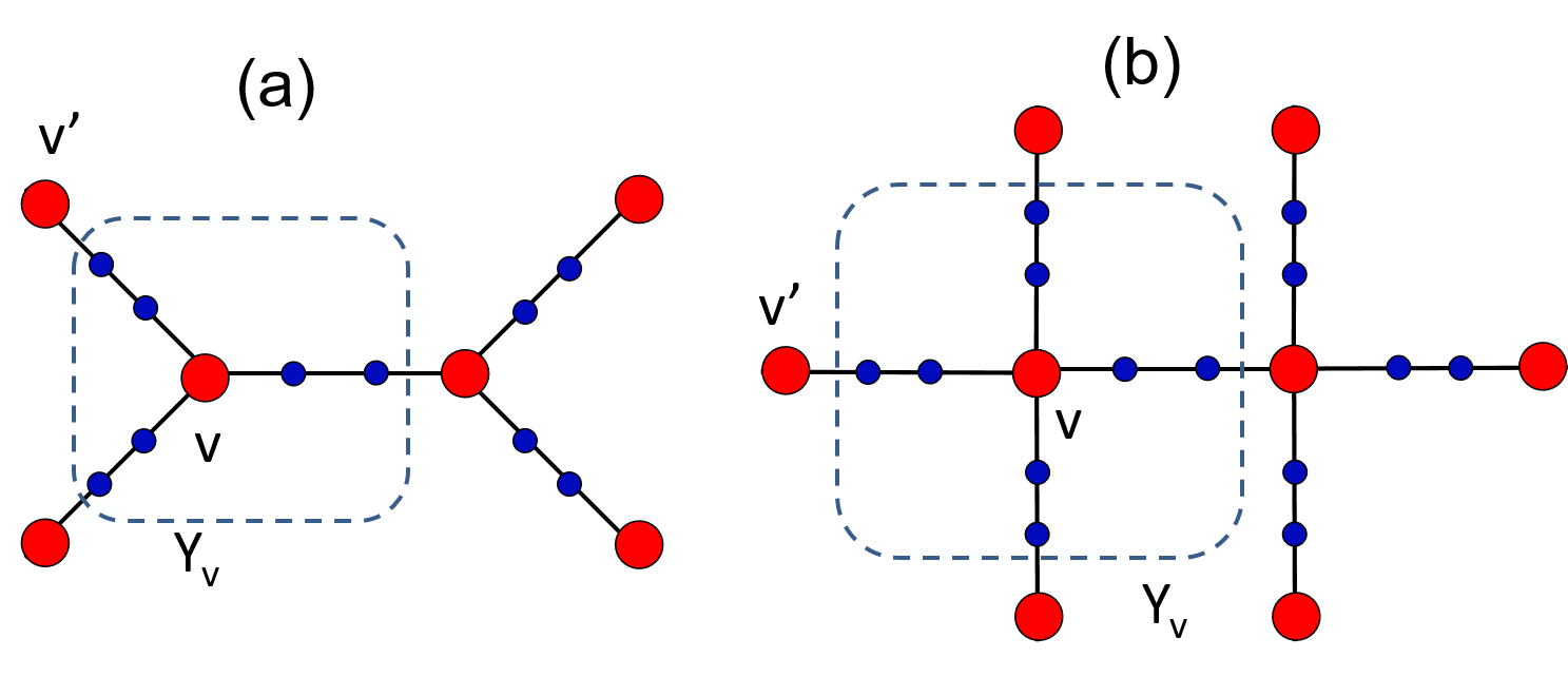 Figure 1
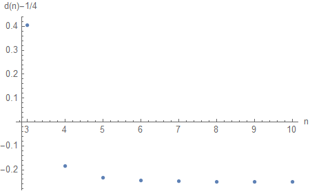 Figure 2
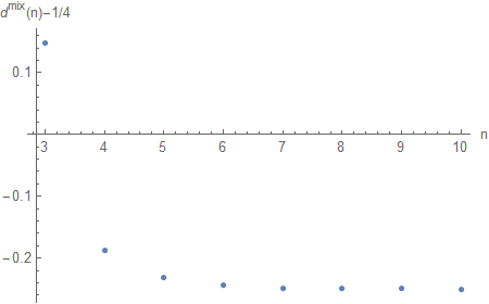 Figure 3
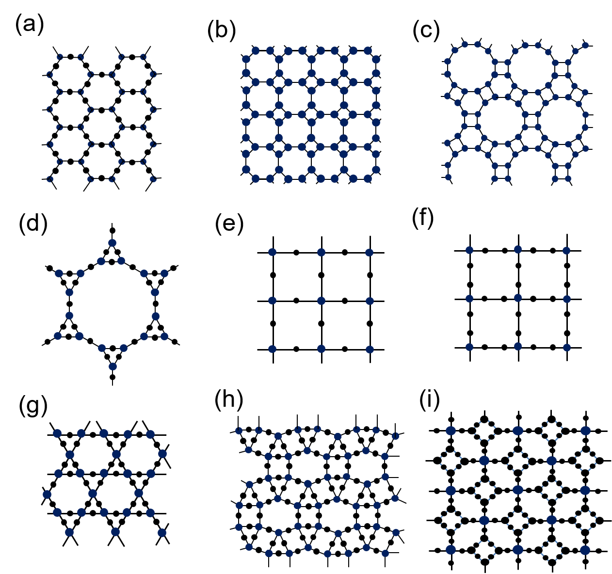 Figure 4
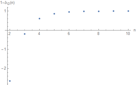 Figure 5
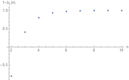 Figure 6
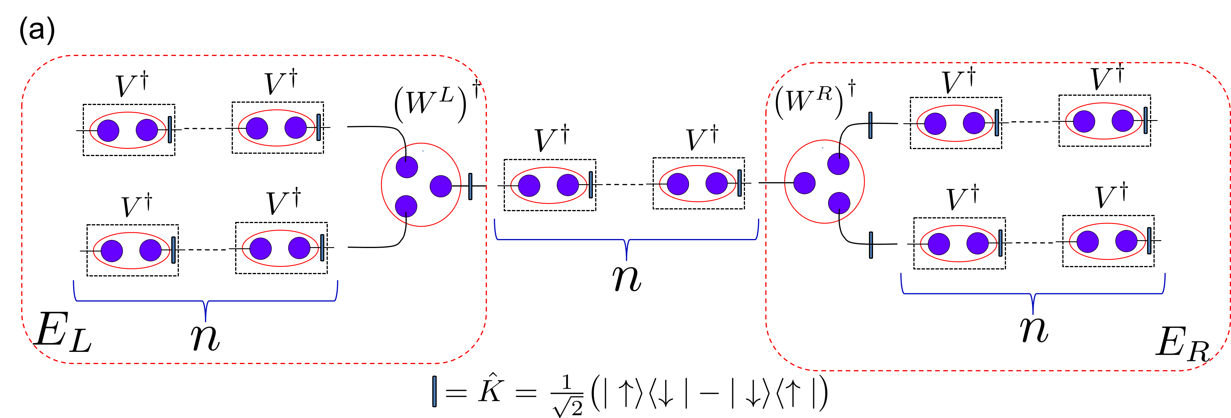 Figure 7
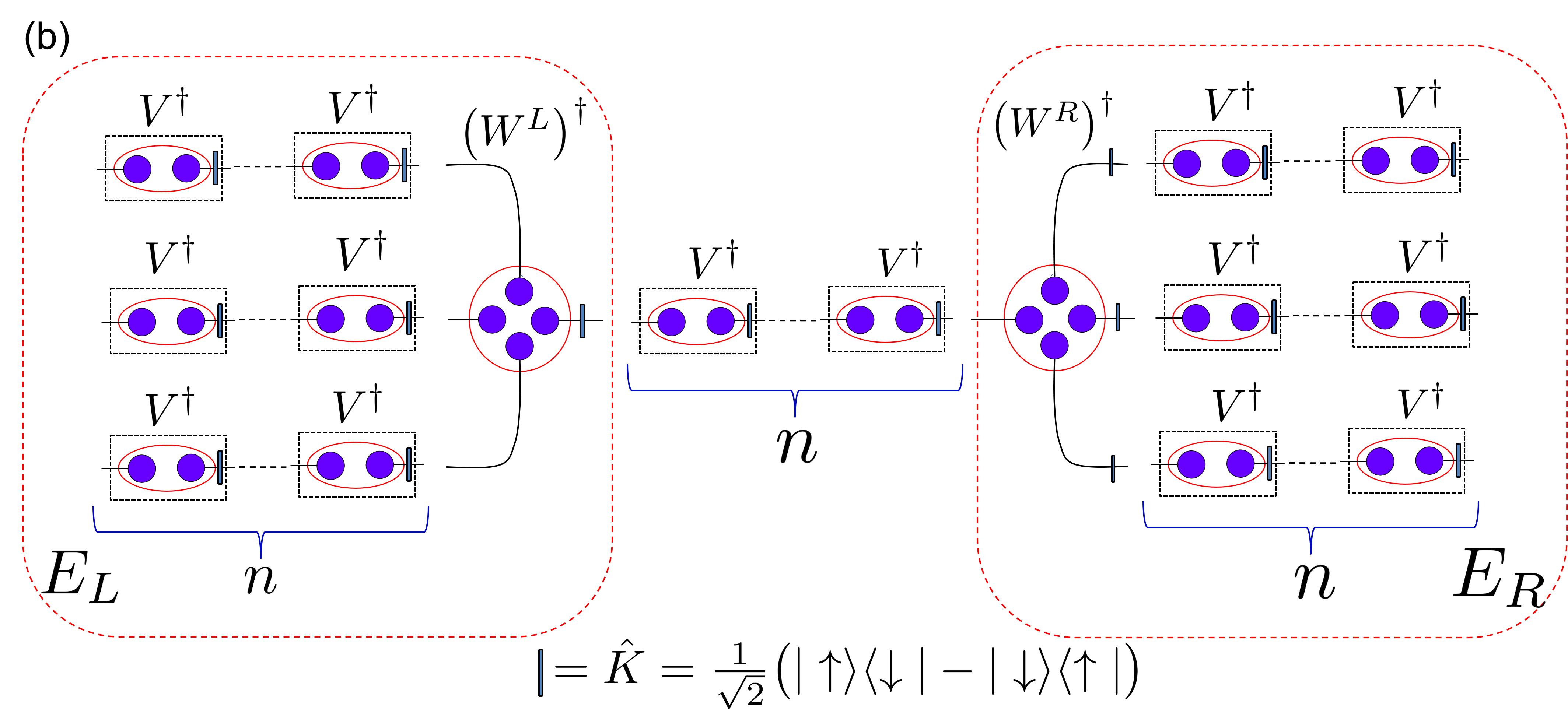 Figure 8
|
|
|
deg. 6 | |||||||
|---|---|---|---|---|---|---|---|---|---|---|
| 1 | 0.4778328889 | 0.5234369088 | 0.5001917602 | 0.6027622993 | ||||||
| 2 | 0.1183378500 | 0.1218467396 | 0.1200794787 | 0.1285855428 | ||||||
| 3 | 0.0384373228 | 0.0389033280 | 0.0386700977 | |||||||
| 4 | 0.0124460198 | 0.0124961718 | 0.0124710706 | |||||||
| 5 | 0.0041321990 |
|
|
|
|
|||||||||
|---|---|---|---|---|---|---|---|---|---|---|---|---|
| 1 | 0.283484861 | 0.170646233 | ||||||||||
| 2 | 0.239907874 | 0.154737328 | 0.197934811 | 0.101463966 | ||||||||
| 3 | 0.207152231 | 0.183265099 |
Peer Reviews
No public reviews on file for this paper yet. If you reviewed it on a platform where reviews are public (OpenReview, ICLR, NeurIPS, ICML), you can paste yours below so the community can read it here.
Videos
No videos yet. Explain this paper in a talk, walkthrough, or lecture? Add one.
AKLT models on decorated square lattices are gapped
Nicholas Pomata
C. N. Yang Institute for Theoretical Physics and Department of Physics and Astronomy, State University of New York at Stony Brook, Stony Brook, NY 11794-3840, USA
Tzu-Chieh Wei
C. N. Yang Institute for Theoretical Physics and Department of Physics and Astronomy, State University of New York at Stony Brook, Stony Brook, NY 11794-3840, USA
Institute for Advanced Compuational Science, State University of New York at Stony Brook, Stony Brook, NY 11794-5250, USA
Abstract
The nonzero spectral gap of the original two-dimensional Affleck-Kennedy-Lieb-Tasaki (AKLT) models has remained unproven for more than three decades. Recently, Abdul-Rahman et al. [arXiv:1901.09297] provided an elegant approach and proved analytically the existence of a nonzero spectral gap for the AKLT models on the decorated honeycomb lattice (for the number of spin-1 decorated sites on each original edge no less than 3). We perform calculations for the decorated square lattice and show that the corresponding AKLT models are gapped if . Combining both results, we also show that a family of decorated hybrid AKLT models, whose underlying lattice is of mixed vertex degrees 3 and 4, are also gapped for . We develop a numerical approach that extends beyond what was accessible previously. Our numerical results further improve the nonzero gap to , including the establishment of the gap for in the decorated triangular and cubic lattices. The latter case is interesting, as this shows the AKLT states on the decorated cubic lattices are not Néel ordered, in contrast to the state on the undecorated cubic lattice.
I Introduction
Affleck, Kennedy, Lieb, and Tasaki (AKLT) constructed a one-dimensional spin-1 chain whose Hamiltonian is rotation-invariant in the spin degree of freedom AKLT1 , but has a spectral gap above the unique ground state, in contrast to the spin-1/2 antiferromagnetic Heisenberg model. This provided strong support for Haldane’s conjecture Haldane83 ; Haldane83b regarding the relation between the spectral gap and spin magnitudes in quantum magnetism. They also generalized the construction to two dimensions AKLT2 , and showed, in particular, that the spin-spin correlation function of the ground-state wavefunction decays exponentially in the honeycomb and the square lattice models. The uniqueness of the ground state in these models was further analyzed by Kennedy, Lieb and Tasaski KLT . There have been a few useful techniques for showing uniqueness of the ground state and gap Fannes1992 ; KLT ; Knabe , which work well in one dimension, but the proof of the nonzero spectral gap has not been established for either of the two 2D AKLT models, even more than three decades after their construction.
Haldane’s conjecture on the spectral property of isotropic chains of integer spins complements the result of Lieb, Schultz and Mattis (LSM) on the properties of chains of half-odd spins, which states that there exists an excited state with energy degenerate with the ground state in the thermodynamic limit LSM . That is the system is either gapless or has degenerate ground states. This LSM theorem was generalized to higher dimensions Oshikawa ; Hastings with each unit cell having half-integer total spin, and the ground state, in addition to the possibility of being gapless or degenerate, can also be a gapped spin liquid that does not break the symmetry. Recently, due to the tremendous progress on topological phases, the LSM theorem has been re-examined in new perspectives, such as symmetry-protected topological (SPT) phases, crystalline symmetry, anomaly, and boundary PoWatanabe17 ; JianBiXu ; Lu ; Cheng ; Shiozaki ; OgataTasaki ; ChoHsiehRyu ; YaoOshikawa . For example, it was conjectured that all LSM-like theorems can be understood from lattice homotopy PoWatanabe17 , and this was very recently generalized to develop a topological theory of LSM theorems in quantum spin systems ElseThorngren .
Unexpectedly, 2D AKLT states have recently emerged as resource for univeral quantum computation (QC) in the framework of the measurement-based quantum computation (MBQC) RB2001 ; BBDR2009 ; RW2012 ; Wei2018 . The spin-3/2 AKLT state on the honeycomb lattice was first shown to provide the appropriate entanglement structure for universal QC Wei2011 ; Miyake2011 , a result subsequently generalized to other trivalent lattices Wei2013 . Before the demonstration of the computational universality of the spin-2 AKLT state on the square lattice Wei2015 , a few decorated lattice structures (with mixed vertex degrees) and the corresponding AKLT states were first considered in Ref. Wei2014 . A partial picture of quantum computation universality in the family of AKLT states is as follows. Any AKLT state residing on a two- or three-dimensional frustration-free regular lattice (no loop with an odd number of sites) with any combination of spin-2, spin-3/2, spin-1, and spin-1/2 that is consistent with the lattice. Higher-spin systems are mainly not included due to technicalities Wei2015 .
Regarding the gap, tensor network methods were employed and the value of the gap in the thermodynamic limit was estimated Garcia-Saez2013 ; Vanderstraeten2015 . A recent breakthrough in the analytic proof was given by Abdul-Rahman et al. Abdul-Rahman2019 , who considered a family of decorated honeycomb lattices and proved that the corresonding AKLT models are gapped for the number of decorated sites being greater than 2; see e.g. Fig. 1a. The associated AKLT states, according to the results of Ref. Wei2014 , are also universal for MBQC, and hence are also of interest, as the non-zero gap implies that preparation of these states via cooling is useful. Additional progress in analytics has also been made by Lemm, Sandvik and Yang on hexagonal chains Lemm2019 , where the quasi-1D AKLT models are also gapped.
We note that the results of Ref. Abdul-Rahman2019 , as argued below, apply directly to other trivalent lattices with decoration, such as the square-octagon , the cross , and the star (Fig. 1b,c&d.) Although the AKLT Hamiltonians are frustration-free, some features in generalized measurement display some frustration, e.g. on the star lattice Wei2013 . The decoration renders the frustrated star lattice non-frustrated and removes the frustration features in the measurement. AKLT states on all these decorated lattices are also universal for MBQC Wei2013 ; Wei2014 .
Here we prove analytically that AKLT models on 2D decorated square lattices possess nonzero spectral gap for , where is the number of spin-1 decorated sites added to each original edge (see e.g. Fig. 1e&f). This result also implies, in addition to the decorated kagome and lattices (Fig. 1g&h), decorated 3D diamond lattices host AKLT models with nonzero spectral gap. AKLT states on the 3D diamond lattice and the associated decorated ones are also universal Wei2014 ; Wei2015 , and the significance is that these 3D resource states are likely to provide fault-tolerance similar to the 3D cluster state RHG . Moreover, proving the spectral gap and knowing its value will be crucial in state preparation and validation protocols.
Using the results from both the decorated honeycomb and square lattice, we also show that AKLT models on decorated lattices whose underlying lattice is of mixed vertex degrees 3 and 4 are also gapped for . We also provide a numerical approach that allows us to study the parameters which bound the gap for , previously thought inaccessible. Our numerical results further improve the nonzero gap to , including the establishment of the gap for in the decorated triangular and cubic lattices, i.e. those whose underlying lattices have vertex degree 6. We also provide much improved lower bounds on the spectral gap for some of the AKLT models. The structure of the remaining paper is as follows. In Sec. II we first review methods used in Ref. Abdul-Rahman2019 . Then in Sec. III we perform the same detailed calculations for the AKLT models on the decorated square lattices. In Sec. IV we make some comments on the other decorated lattices. In Sec. V, we describe our numerical methods which improve all the above gappedness scenarios to . Finally in Sec. VI we make some concluding remarks.
II Review of prior methods and results
Here we briefly review the key points that enable the proof of the spectral gap for AKLT models on the decorated honeycomb lattice in Ref. Abdul-Rahman2019 ; see Fig. 1 for one such illustration with , as well as other lattices. We will try to use the same symbols as in Ref. Abdul-Rahman2019 as much as possible, but may have some slight differences. Consider an original lattice (e.g. honeycomb or square lattice) and its decorated version in which each edge of has been decorated with spin-1 sites. Let denote the edge set of the decorated lattice. The AKLT model Hamiltonian defined on is
[TABLE]
where is a projection onto the total spin subspace of the two spins linked by the edge , and denotes the sum of the coordination numbers (i.e. vertex degrees and ) of the two spins and linked by edge .
Instead of directly using the AKLT Hamiltonian, Ref. Abdul-Rahman2019 first considers a slightly modified one:
[TABLE]
where is the AKLT Hamiltonian on the set of vertices of the decorated lattice , is the coordination number ( for the honeycomb) and denotes the edges connecting vertices in ; see Fig. 2 for illustration. It has a few terms in missing, i.e., those terms on the edges containing the last spin-1 site on edge and the next site . So we have an inequality
[TABLE]
However, instead of , Ref. Abdul-Rahman2019 also considers a slight modification
[TABLE]
where is the orthogonal projection onto the range of . The kernel of is the ground space of , i.e., . Then it is shown that
[TABLE]
where is the smallest nonzero eigenvalue of (or equivalently the spectral gap of the small system ) and is the usual operator norm of (or equivalently the largest eigenvalue of , since is non-negative).
The strategy is to prove is gapped. By squaring , we find that
[TABLE]
where for those and not on the same edge is non-negative and is dropped, resulting in the last inequality. If one can find the minimum positive number such that , then
[TABLE]
where (the subscript is added to ) and is the coordination number of the underlying lattice (e.g. for the honeycomb and for the square lattice). If , then one proves that has a spectral gap above the ground state(s).
Therefore, most of effort goes into finding or an upper bound. A relation that was used to this end in Ref. Abdul-Rahman2019 is Lemma 6.3 from Ref. Fannes1992 for a pair of projectors and :
[TABLE]
where denotes the projection onto the joint subspace . When we apply this relation to (9), becomes an upper bound on , i.e., . In particular, in Prop. 1 below, we determine that . In Sec. V below we will additionally develop techniques to compute exactly.
Using the above Lemma and employing tensor-network approaches, the authors of Ref. Abdul-Rahman2019 show elegantly that
[TABLE]
where
[TABLE]
In the above expressions, is the quantum channel, or equivalently the transfer matrix, obtained from the tensors associated with the ‘left’ set of vertices and (via tensors ) is associated with the ‘right’ set of vertices . See also Figs. 2 and 3 for illustration. More precisely, the channels are defined as follows,
[TABLE]
Note that by examining the derivations in Ref. Abdul-Rahman2019 , the operator norms associated with and holds both for the norm with respect to -norm of and and for that w.r.t. the Hilbert-Schmidt norm of matrices. However, since the latter norm is larger for the former, the former norm presents a better bound.
Moreover, two specific matrices are introduced: and ( here equaling ), and and are their respective minimum eigenvalues. For the proof, we highly recommend Ref. Abdul-Rahman2019 to the readers.
III Analysis of spectral gap
The spin-2 entity residing on each square lattice site is composed of four virtual qubits projected onto their symmetric subspace, and the mapping between the physical spin-2 degrees of freedom and the those in the symmetric subspace is as follows,
[TABLE]
where ’s are eigenstates of spin-2 operators with eigenvalue ’s. If we consider one square lattice site on the left, then there are corresponding tensors for , which are
[TABLE]
Because the AKLT state is formed from projecting virtual singlet pairs via symmetric projectors, we obtain the local tensors describing the spin-2 site on the left as , where , and they are given as follows,
[TABLE]
See also Fig. 3b for illustration of the local lattice structure and the corresponding tensors. From these, one can easily check that
[TABLE]
and one can define a quantum channel
[TABLE]
(We note that one could re-scale ’s so as to make the right hand side of Eq. (17) be , but we won’t do that here.) One also finds that
[TABLE]
where is the projector to the 3-qubit symmetric subspace. At this point it is useful to introduce the two W states used in quantum information so as to simplify the notation,
[TABLE]
The associated dual quantum channel is defined as , which maps any three-qubit density matrix to a one-qubit density matrix, and can be written as (assuming is Hermitian for simplicity)
[TABLE]
where the four coefficients c{\color[rgb]{.5,0,.5}{}_{i}} are
[TABLE]
Similar to the decorated honeycomb case, is invariant in permuting , and in the special form , and this can be used to simplify some calculations. Let us use the lower-case to denote the spin-1/2 operators and recall that . One can then by direct calculation show that
[TABLE]
To proceed further, it is useful to introduce
[TABLE]
and by direct calculation one can re-write Eq. (19) as
[TABLE]
which will allow us later to deduce from the actions of in Eqs. (27) by fixing the overall scale.
It is convenient to express the channel and its dual in the form of a matrix, sometimes called the superoperator form or the Liouville formalism. Thus, any matrices, such as , that the channels act on will be written in terms of vectors, such as . Moreover the inner product between two such ‘vectors’ becomes . Note that in this definition . Then exploiting the permutation invariance of , one can employ the trick used in Ref. Abdul-Rahman2019 , by using the action of the dual channel in Eqs. (27) and fixing the overall scale via Eq. (29), to deduce the action of and write it in the ‘superoperator’ form as
[TABLE]
where we have suppressed the symbols. It is also possible to calculate directly from its definition in Eq. (18), but the trick above helps to express in terms of the sum of the product forms for the superoperators.
From the results of Ref. Abdul-Rahman2019 , the channel along decorated spin-1 sites,
[TABLE]
is calculated to be
[TABLE]
and thus the combined channel from the left is (see Fig. 3)
[TABLE]
where was introduced in Eq. (28) and here we introduce its vectorized form , as well as and .
Next, we consider the operator , and obtain it in the matrix form (instead of )
[TABLE]
One can diagonalize and obtain its spectrum (noting has eigenvalues )
[TABLE]
Therefore, the smallest eigenvalue of is
[TABLE]
The transfer operator is completely positive choi , since it is constructed from Kraus operators via Eqs. (18), (31) and (33), or alternatively it can be checked by directly diagonalizing the corresponding Choi matrix choi . Hence, it is also 2-positive, and from a Cauchy-Schwarz inequality for 2-postive maps Paulsen , we have that
[TABLE]
From this we can calculate the associated and obtain
[TABLE]
where a(n)=\big{|}\big{|}E^{n}-|\openone\rangle\rangle\langle\langle\rho_{1}|\big{|}\big{|} was previously obtained in Ref. Abdul-Rahman2019 to be ; but one can also calculate directly from Eq. (32).
Next, we examine the channel coming from the right square-lattice site. The onsite tensors are defined as , and one finds that
[TABLE]
From these, we see that is dual to the channel , i.e., . Therefore, using the superoperator formalism, is dual to , i.e. ; this shows that . Moreover, the operator , and therefore we have that the relation between the minimum eigenvalues of and is . We therefore obtain
[TABLE]
The injectivity of the mappings and for the corresponding matrices , , to the respective quantum states,
[TABLE]
depends on whether and , respectively; see Ref. Abdul-Rahman2019 . In the above equations, and denote tensors from the left and right sides, respectively, and are basis states for the left and right sides, respectively, and denotes the tensor for one spin-1 site that decorates the edge ( is the total number of such sites); see Fig. 3. We have checked that , and are injective for ; see Figs. 4 and 5. From Ref. Abdul-Rahman2019 , , and it was shown that the important quantity is upper bounded by
[TABLE]
Here, if then the corresponding AKLT model has a finite gap, whereas if it is undecided. Thus, we have
[TABLE]
We can thus prove that the AKLT models on the decorated square lattice are gapped with , as shown in Fig. 6. But the analytics cannot say anything about .
Since is only an upper bound on , we also performed numerical calculations directly for for both the decorated honeycomb and square lattice (as well as one with mixed degrees), and confirmed that for both and the AKLT models are also gapped. The numerical results are shown in Table 1. We describe our methods in Sec. V.
IV Comments on other lattice
IV.1 Other trivalent lattices
Since the proof in the decorated honeycomb case Abdul-Rahman2019 only relies on the local structure of the two vertices on the underlying lattice and the corresponding tensors (see Fig. 3 for illustration), a moment of thought will convince one that it also holds exactly for other trivalent lattices with decoration on their edges; see Fig. 1 for illustration of other lattices. (However, this does not necessarily mean that the actual values of the gap will be identical.) Therefore for all trivalent lattices, which can be of any dimensions, such as 3D, the AKLT models on the corresponding decorated lattices will also be gapped if (using the results on the decorated honeycomb in Ref. Abdul-Rahman2019 ), where again is the number of spin-1 sites added to decorate an edge. In fact, for each undecorated edge, the number of decorated sites can be different, and the corresponding AKLT model will still be gapped as long as . Numerically these bounds are improved to ; see below.
IV.2 Other lattices of vertex degree 4
By the same token, since we have proven that the AKLT models on the decorated square lattices are gapped if , this will also hold for any other decorated lattices, whose undecorated vertex degree is 4; see Fig. 1g&h for illustration of such lattices. Numerically these bounds are also improved to . AKLT states on the 3D diamond lattice (also four-valent) and the associated decorations are also universal Wei2014 ; Wei2015 , and the significance is that these 3D resource states are likely to provide fault tolerance similar to the 3D cluster state RHG . Therefore, the decorated diamond lattices host AKLT models that are gapped for , and the corresponding ground states are also universal and likely provides topological protection for MBQC.
IV.3 Other lattices of fixed vertex degree
We conjecture that for any lattices of fixed vertex degree, the AKLT models on the corresponding decorated lattices will be gapped, as long as is large enough. The intuition comes from that for large , it is essentially many long spin-1 AKLT chains incident on some vertices, which act as local perturbations. For sufficiently large, the perturbation is of measure zero as . Of course, this is only an intuition, rather than an actual proof.
IV.4 Lattices of mixed vertex degrees
A natural extension to examine is those AKLT models residing on decorated lattices whose undecorated ones are of mixed vertex degrees. It is likely that they will be gapped as long as is sufficiently large.
Let us consider the lattice (i) in Fig. 1, whose underlying lattice has mixed vertex degrees of 3 and 4. Take the left original site to be of degree 3 and the right original site of degree 4. We have to evaluate , , , and , and they can be obtained partly from the honeycomb case and partly from the square lattice case,
[TABLE]
Thus, we obtain the corresponding function for the mixed-degree lattice,
[TABLE]
We see that the AKLT models are gapped for for the decorated lattices, as checked in Fig. 7. Numerically these are improved to ; see Table 1.
V Basis for Numerical Methods
Here we explain our numerical approach for producing the values of in Table 1, which was derived based on Lemma 6.3 of Ref. Fannes1992 . The analytical results in the previous sections provide only upper bounds on , as inequalities such as operators norms and Schwarz inequalities were used in deriving, e.g., Eq. (11). As we have seen, the analytics can only establish a nonzero gap for , but our numerical evaluation of was able to push the gappedness to .
We begin by noting part (1) of the Lemma, which determines that
[TABLE]
where projects onto the intersection of images and, likewise, projects onto the sum , or . From here on we will use and rather than their complements, which will prove useful because and are high-dimensional projectors and their complements are low-dimensional.
Here we also review the findings that lead the source to part (2) of the Lemma. In doing so, we will diverge from the source by not quotienting out and (i.e. setting and ), as we ultimately will be working partly within those spaces. We consider the eigenvalue equation
[TABLE]
Clearly, as and are Hermitian operators whose eigenvalues belong to , the range of possible values of is . Moreover, we note that corresponds exactly to the subspace , whereas corresponds exactly to the subspace . The remaining eigenspaces must lie within the mutual orthogonal complement of these spaces,
[TABLE]
noting that the explicit exclusion of from and means that the above sum is a direct sum.
Therefore, for , we can uniquely write for and . In particular we can rewrite Eq. (58) as
[TABLE]
and arrive at
[TABLE]
which we can rewrite as
[TABLE]
We see immediately that . Moreover, since we have constructed , we immediately have . Thus, we can for example take and apply to both the right and left,
[TABLE]
That is, , and consequently, and .
From this we can directly compute
[TABLE]
Such direct calculation also gives us and . In particular, consideration of individual eigenspaces gives us
[TABLE]
We will then follow the original proof of part (1) of the Lemma in demonstrating
Proposition 1
The inequality
[TABLE]
is optimized by . In particular, is the least nontrivial eigenvalue of .
The operator norm is equivalent to the supremal real value of for unit ; in particular optimizing and implies that and . In finding , we note that vanishes on both and ; i.e. is orthogonal to these spaces and in particular . Likewise, the Hermitian transpose vanishes on and , so that we should find ; in particular, . Noting , thus we can write and . It follows that
[TABLE]
Moreover for any eigenvector of with eigenvalue , decomposed as above into , . In particular, this implies that , as and have the same norm when :
[TABLE]
for ; that is .
Therefore, determining is equivalent to determining the least nontrivial eigenvalue of . We now demonstrate that we can simplify and, by extension, reduce the complexity of this calculation.
Consider a projector , with the properties (i.e. ) and . (In particular, we will be interested in a projector defined on the sites .)
Proposition 2
For an eigenvector of with eigenvalue , , .
As above, we write with and , so that and ; in particular . Manifestly as ; meanwhile, since we can write
[TABLE]
We use to project onto a lower-dimensional subspace ; that is we take , for and . We set and . That and are projectors follows directly from the fact that and commute with . Moreover,
Proposition 3
**
We do this by examining the spectrum of , as in Prop. 1. Since commutes with and , we find that
[TABLE]
that is, for any eigenvector of , is an eigenvector of with the same eigenvalue. Put otherwise, the spectrum of is a subset of that of . Then, by Prop. 2, only the degeneracies of eigenvalues 0, 1, and 2 are affected; in particular the least nontrivial eigenvalue is preserved.
We additionally note that, for a fourth projector commuting with and and satisfying , satisfies the same hypotheses for and . Decomposing , , we can therefore move to a still smaller space and perform our analysis on and . The method we use to efficiently exploit these conclusions is as follows footnote :
Determine as follows:
- (a)
Construct the tensor corresponding to the portion of the AKLT state defined on , containing both physical and virtual indices (in the honeycomb-lattice case, physical and 3 virtual; in the square-lattice case, physical and 4 virtual indices). 2. (b)
Collect the physical and virtual indices, in order to turn the representation into a matrix . 3. (c)
Using the singular-value decomposition (written such that is full-rank), it follows that . 2. 2.
Taking , we can repeat this process to define isometries on , on , and on . 3. 3.
Write and (as it may be prohibitively memory-intensive to represent even and in full). 4. 4.
Then and can be used to extract by diagonalizing .
We applied the above procedure to four different types of lattices, and we found that the AKLT models are gapped for for the decorated lattices, as shown in Table 1. This includes those whose underlying lattices are of degree 6, such as the triangular lattice and even the cubic lattice. The AKLT model on the cubic lattice is interesting, as the ground state, i.e. the AKLT state, is Néel ordered Parameswaran . By decorating the cubic lattice with a few spin-1 sites on every edge, the Néel order is removed, as gapless Goldstone modes must be present in the antiferromagnetic case. The results in Ref. Wei2014 about quantum computational universality for the AKLT family only apply to lattices of vertex degrees equal to or less than 4. But for these 3D decorated AKLT states, we suspect that they are also universal for MBQC.
V.1 Lower bounds on the gap
The lower bound on the gap of the AKLTmodel on the decorated honeycomb can be estimated via Eq. (5) and is given by
[TABLE]
shown in Ref. Abdul-Rahman2019 . The analytic bound of was used, and together with this yielded a lower bound of gap: for the decorated honeycomb lattice. Of course, this can be improved by using the numerical value for from Table 1, and we obtain , which is four times more than orginally found.
An additional improvement can be made by using a slightly different inequality from Eq. (5):
[TABLE]
where is defined to be the smallest nonzero eigenvalue of , which is similar to in Eq. (2), but is instead defined as
[TABLE]
where denotes the set of edges incident on the site on the original, undecorated lattice. The inequalites of Eq. (70) arise naturally due to the fact that
[TABLE]
Thus the new lower bound on the gap is
[TABLE]
where is the appropriate coordination number from the underlying lattice (one should take the largest one if the lattice is of mixed degree). We show in Table 2 a few lower bounds on the gap. For the decorated honeycomb example considered above, the lower bound on the gap is improved to .
At this point, we would like to entertain the idea of extrapolating the lower bound from & linearly to and . Doing this, we would obtain (extrapolated) and (extrapolated). The latter value is interesting, as it is consistent with the numerical gap value of the model on the honeycomb lattice , obtained in Ref. Garcia-Saez2013 using tensor-network methods. Of course, there is no basis for why such an extrapolation should be valid.
VI Concluding remarks
We have followed the elegant approach by Abdul-Rahman et al. Abdul-Rahman2019 and proved analytically that the decorated square lattices with host AKLT models with finite spectral gap, similar to the results of the decorated honeycomb case. Our numerical approach extends beyond what was accessible previously and allows to show that the AKLT models on both decorated lattices are gapped even for and . The results of a nonzero spectral gap also hold for any other decorated lattices of which the underlying lattices are of fixed vertex degree 3 or 4. But we have also commented on other lattices. In particular, using the results from both the decorated honeycomb and square lattice, we also show analytically that AKLT models on decorated lattices where the underlying lattice has mixed vertex degrees 3 and 4, are also gapped for . This is improved numerically to . Regarding the spectral gap for the AKLT models on the undecorated honeycomb or square lattice, we also share the same view as the authors of Ref. Abdul-Rahman2019 , i.e. to establish their spectral gap will require a different and maybe novel approach. However, some insight may be obtained if one can make progress analytically on the cases of and in particular whether case is gapped or not, for which we strongly suspect that it is gapped.
Our numerical results also show the nonzero gap for in the decorated triangular and cubic lattices. Observing the decaying trend of on in the previous analysis, we believe that the nonzero gap should exist for all . One can carry out the analytic procedure for the degree-6 case. The calculations are expected to be more tedious but likely straightforward. Such a result is interesting for the cubic lattice, as this shows the AKLT states on the decorated cubic lattices are not Néel ordered, in contrast to the state on the undecorated cubic lattice. Naively, decoration using spin-1 sites introduces more quantum fluctuations than those from spin-3 sites and destroys the Néel order. In contrast, the ground state of the spin-1/2 Heisenberg model on the cubic lattice is antiferromagnetically ordered, despite the seemingly larger quantum fluctuations from such low-spin magntude entities. The phenomena of the suppresion of order, as well as the other kind of suppression—of frustration, as mentioned in the Introduction, may be of interest for futher exploration.
AKLT models that have spin rotational symmetry but a deformation that breaks the full SO(3) symmetry were considered, such as the deformed AKLT models in Refs. Niggemann1997 ; Niggemann2000 . Can we employ a similar approach to prove the spectral gap for the deformed models on the decorated lattices? It is also possible that ideas from tensor network can be useful, such as those in Refs. Schuch2011 ; Darmawan2016 . Some deformed AKLT states were also previously shown to provide a universal resource for MBQC within some finite range of deformation Darmawan2012 ; Huang2016 . These deformed models also have interesting phase diagrams Niggemann1997 ; Niggemann2000 ; Hieida1999 ; Huang2016 ; Pomata2018 . It is worth mentioning that some related 2D Hamiltonians interpolating the AKLT and the cluster-state models were also shown to have finite spectral gap Darmawan2016 , but the spectral gap in the exact AKLT limit is still not proved.
Acknowledgements.
This work was supported by the National Science Foundation under grants No. PHY 1620252 and No. PHY 1915165. T.-C.W. thanks Bruno Nachtergaele for useful communication regarding the issue of the norms.
The reference list from the paper itself. Each links out to its DOI / PubMed record.
- 1(1) I. Affleck, T. Kennedy, E. H. Lieb, and H. Tasaki, Rigorous results on valence-bond ground states in antiferromagnets, Phys. Rev. Lett. 59 , 799 (1987).
- 2(2) F. D. M. Haldane, Continuum dynamics of the 1-d Heisenberg antiferromagnet: identification with the O(3) nonlinear sigma model, Phys. Lett. 93 , 464 (1983).
- 3(3) F. D. M. Haldane, Nonlinear field theory of large-spin Heisenberg antiferromagnets: semiclassically quantized solutions of the one-dimensional easy-axis Neel state, Phys. Rev. Lett. 50 , 1153 (1983).
- 4(4) I. Affleck, T. Kennedy, E. H. Lieb, and H. Tasaki, Valence Bond Ground States in Isotropic Quantum Antiferromagnets, Comm. Math. Phys. 115 , 477 (1988).
- 5(5) T. Kennedy, E. H. Lieb, and H. Tasaki, A two-dimensional isotropic quantum antiferromagnet with unique disordered ground state, J. Stat. Phys. 53 , 383 (1988).
- 6(6) M. Fannes, B. Nachtergaele, R.F. Werner, Finitely Correlated States on Quantum Spin Chains, Commun. Math. Phys. 144 , 443 (1992).
- 7(7) S. Knabe, Energy gaps and elementary excitations for certain VBS-quantum antiferromagnets, J. Stat. Phys. 52 , 627 (1988).
- 8(8) E. H. Lieb, T. Schultz, and D. J. Auerbach, Two soluble models of an antiferromagnetic chain, Ann. Phys. (N.Y.) 16 , 407 (1961).