Return amplitude after a quantum quench in the XY chain
Khadijeh Najafi, M. A. Rajabpour, Jacopo Viti

TL;DR
This paper derives an exact formula for transition amplitudes in the quantum XY chain, analyzes return amplitudes for specific states, and explores finite-size effects and dynamical phase transitions.
Contribution
It provides a new exact analytical expression for transition amplitudes and investigates finite-size effects and dynamical phase transitions in the XY chain.
Findings
Exact formula for transition amplitudes between eigenstates.
Analytical expression for return amplitude of polarized and Nél states.
Finite-size effects and traversal phenomena depend on initial state and system size.
Abstract
We determine an exact formula for the transition amplitude between any two arbitrary eigenstates of the local -magnetization operators in the quantum XY chain. We further use this formula to obtain an analytical expression for the return amplitude of fully polarized states and the N\'eel state on a ring of length . Then, we investigate finite-size effects in the return amplitude: in particular quasi-particle interference halfway along the ring, a phenomenon that has been dubbed traversal~\cite{FE2016}. We show that the traversal time and the features of the return amplitude at the traversal time depend on the initial state and on the parity of . Finally, we briefly discuss non-analyticities in time of the decay rates in the thermodynamic limit , which are known as dynamical phase transitions.
Click any figure to enlarge with its caption.
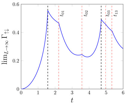 Figure 1
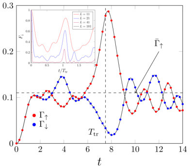 Figure 2
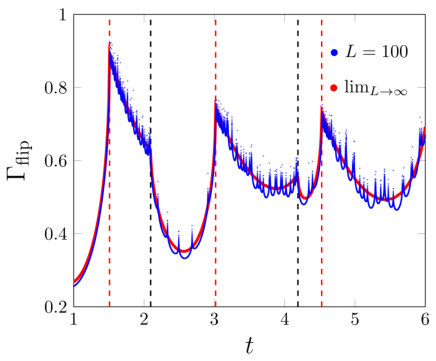 Figure 3
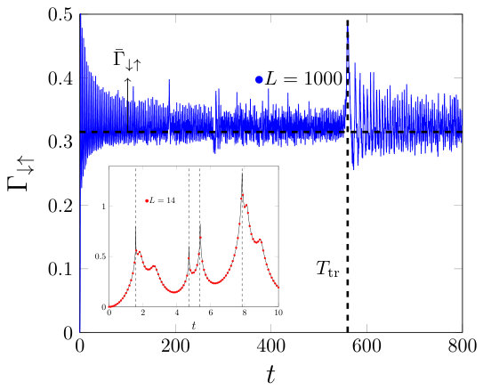 Figure 2
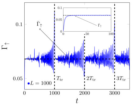 Figure 5
Peer Reviews
No public reviews on file for this paper yet. If you reviewed it on a platform where reviews are public (OpenReview, ICLR, NeurIPS, ICML), you can paste yours below so the community can read it here.
Videos
No videos yet. Explain this paper in a talk, walkthrough, or lecture? Add one.
Return Amplitude after a Quantum Quench in the XY Chain
Khadijeh Najafi
Department of Physics, Virginia Tech, Blacksburg, VA 24061, U.S.A
M. A. Rajabpour
Instituto de Física, Universidade Federal Fluminense, Av. Gal. Milton Tavares de Souza s/n, Gragoatá, 24210-346, Niterói, RJ, Brazil
Jacopo Viti
International Institute of Physics, UFRN, Campos Universitário, Lagoa Nova 59078-970 Natal, Brazil
ECT, UFRN, Campos Universitário, Lagoa Nova 59078-970 Natal, Brazil
Abstract
We determine an exact formula for the transition amplitude between any two arbitrary eigenstates of the local -magnetization operators in the quantum XY chain. We further use this formula to obtain an analytical expression for the return amplitude of fully polarized states and the Néel state on a ring of length . Then, we investigate finite-size effects in the return amplitude: in particular quasi-particle interference halfway along the ring, a phenomenon that has been dubbed traversal FE2016 . We show that the traversal time and the features of the return amplitude at the traversal time depend on the initial state and on the parity of . Finally, we briefly discuss non-analyticities in time of the decay rates in the thermodynamic limit , which are known as dynamical phase transitions.
I Introduction
A prominent theoretical tool to investigate non-equilibrium phenomena in many-body systems is the quantum quench. In the original formulation of the problem Silva , a quantum system is prepared in the ground state of a translation invariant Hamiltonian depending on a control parameter. Such a parameter is suddenly modified (quenched) so that the unitary time evolution of the quantum state is governed by the post-quench Hamiltonian.
In low dimensions, tailored field theoretical CC2006 ; CC2007 ; FM ; SE ; BES ; Delfino2014 ; DV2017 ; KZ ; TM , free fermionic Sac ; Muk07 ; CEF2011 ; CEF2011a ; CEF2011b ; Igloi2012 ; Bucciantini2014b and Bethe Ansatz techniques QA ; DeNa ; DeNa2 ; FCEC14 ; Poz ; Proz ; MPC ; BPC have been exploited for analytical investigation of the unitary dynamics after the quench. For reviews we refer to the special issue CEM and Eis_rev ; Pol_rev .
There is a firm consensus CEM that macroscopic subsystems of a closed infinite system can equilibrate at late times to a stationary quantum density matrix. For one-dimensional integrable models, such a density matrix is a reduced density matrix obtained from a Generalized Gibbs Ensemble (GGE) GGE_rigol ; GGE_rigol2 . This recent theoretical study—especially after KW —has been motivated and boosted by the experimental implementation with ultra-cold atoms of one-dimensional systems which are in almost perfect isolation from the external environment coldatoms .
In the framework pedagogically reviewed in FE2016 , subsystem relaxation towards equilibrium can only occur if the volume of the system is infinite. In a finite system, the energy spectrum might be discrete and the wave function recur Bocchieri1957 , although with periods growing exponentially with the system size. More importantly, in an integrable model, finite size effects can prevent relaxation to a stationary state much earlier Igloi2000 than a recurrence takes place. Suppose that an integrable spin chain is quantized on a ring of length and is a maximal LR effective propagation velocity for the quasi-particles. Then, qualitatively, quasi-particles emitted in pairs CC2006 can interfere halfway along the ring at instants of time multiples of , which is . Following Sec. 5.2 in FE2016 , we will call the time around which quasi-particle interference in finite volume prevent relaxation to a time-independent stationary state, the traversal time.
An observable that diagnoses finite-size effects and can provide a quantitative estimate of is the return amplitude or fidelity Quan2006 ; Yuan2007 ; Rossini2007 ; S2008 ; Zhong2011 ; Zanardi2011 ; MC12 ; Santos14 ; DeLuca14 ; PS14 ; Santos15 ; Mazza2016 ; Poz_echo ; Poz_echo2
[TABLE]
where is the many-body initial state and , the post-quench Hamiltonian. In particular, destructive or constructive quasi-particle interference is detectable in the logarithm of the return amplitude ; hereafter, we will refer to as the decay rate. For the quenches considered in this paper, the decay rate relaxes in infinite volume at later times—or rather in a window —to a constant Z2010 , that is the limit
[TABLE]
exists and can be calculated. For finite large instead, when approaching the traversal times, the amplitude of the decay rate oscillations around increases; see Fig. 1 for an example that will be discussed in detail. At each traversal time, moreover, the decay rate exhibits local maxima or minima, which signal that the system, being finite, cannot relax to a time-independent stationary state. Actually, after many traversals, the time average of the finite volume return probability converges to its value in the diagonal ensemble Z2010 ; F13 ; LV ; Mazza2016 , . A correspondent decay rate in infinite volume can be extracted which generally differs Z2010 ; F13 from defined earlier; cf. Eq. (48) in Sec. IV of this paper.
Finite-size effects in the return amplitude have been investigated in the last years Happola ; Montes2012 ; Sharma2012 ; Rajak2014 ; KR2017 ; Jafari2017 ; Damski ; Jafari2019 seeking for a revival—i.e. an instant at which —of the initial wave function. However, as pointed out in FE2016 and stressed once more in the Sec. IV of this paper, at the traversal time there is usually not a bona fide revival of the quantum state. The return amplitude remains always exponentially small with respect to the system size, i.e. even for reasonably large but finite systems. Indeed a necessary condition for a revival in a time which is of a state that has an exponential number of non-zero overlaps with the eigenenergy basis, is the fact that the many-body spectrum, in a certain energy unit , is integer spaced. This can happen, for instance, in the continuum limit if non-interacting quasi-particles quantized on a cylinder have a linear dispersion relation. In a lattice model however, the quasi-particles dispersion is never linear on the whole Brillouin zone. The absence of revivials in the critical XY chain was investigated in detail in KR2017 . As a matter of fact, up to now, one can observe physically relevant B2017 examples of revivals only within the context of conformal invariant field theories DS2011 ; Cardy_echo .
The decay rate of the return amplitude in the thermodynamic limit can also show non-analyticities in time that have been dubbed dynamical phase transitions Heyl2013 and are the focus of an intense research activity Pollmann2010 ; Karrasch2013 ; AS ; SB ; Gullo2015 ; Lupo2016 ; Pollmann2016 ; Heyl2017 ; H1 ; H2 ; H3 ; S16 ; BD18 ; TH18 ; Sirker18 ; H4 ; for a recent comprehensive survey we refer to the review Heyl_rev . The nature of such singularities and a possible link with the statistical mechanics are still unsettled AS ; Poz_echo , although they have been observed experimentally DPT_exp2 ; DPT_exp ; see also the viewpoint in G17 .
In this paper, we will study both the finite size effects and the non-analyticities in the thermodynamic limit for the return amplitudes in the XY chain LMS . We will focus on initial states that are eigenstates of the local -magnetization operator; examples will include fully polarized states and the Néel state. These initial states are Gaussian—i.e. the Wick theorem holds KRV2018a ; BTC2018 —and allow local relaxation in the thermodynamic limit to a stationary state SC ; BTC2018 ; moreover, they are experimentally relevant DPT_exp ; DPT_Monroe .
Our analytical results are based on a new formula for the matrix elements of the evolution operator associated with a quadratic fermionic Hamiltonian, which we will derive in Sec. II; see Eq. (14). In Sec. III, we specialized this result to calculate return amplitudes in the XY chain. In Sec. IV, we provide detailed physical applications of the formalism and analyze the finite-size effects and the singularities in the thermodynamic limit in the decay rate of a fully polarized state and of the Néel state. We will then calculate the traversal times and show that they are initial state dependent; we will also determine the instants of time at which singularities in the thermodynamic limit of the decay rate show up. Our conclusions are gathered in Sec. V, and an appendix completes the paper.
II Return amplitude in free fermionic chains
The aim of this section is the derivation of a formula to calculate the Return Amplitude (RA) for an arbitrary many-body state time-evolving with a free fermionic Hamiltonian. We start by considering the following quadratic Hamiltonian in the real space ( denotes transposition below)
[TABLE]
where A and B are real symmetric and antisymmetric matrices, respectively. The -dimensional column vector c contains the annihilation operators with . Their Hermitian conjugates are and canonical anticommutation relations hold. Transposition of column vectors is understood if required to define a fermionic quadratic form, such as in Eq. (1) or Eqs. (10)-(12). Following Balian and Brezin Balian1969 , we introduce the -dimensional column vector . The evolution operator acts linearly on the vector as
[TABLE]
where the matrix T is obtained by applying the Baker-Campbell-Hausdorff formula (cf. appendix A)
[TABLE]
The blocks () can be written down explicitly if the free fermionic system is translation invariant; in the next section we will provide a physical example. As anticipated in Sec. I, given a quantum state , its RA is defined by
[TABLE]
If is an eigenstate of the local fermion occupation numbers, a determinant representation for can be obtained through the following route. First, we factorize the evolution operator à la Balian-Brezin Balian1969 as
[TABLE]
where X, Y, Z can be calculated from the four blocks of the matrix T in Eq. (3)
[TABLE]
The Balian-Brezin factorization is briefly outlined in the appendix A; here, we only remark that X and Z are complex antisymmetric matrices. The decomposition (5) is suitable for a coherent state representation of the RA, for analogous manipulations of other quantum matrix elements see also Mizusaki13 . Coherent fermionic states are introduced in the usual way through a set of anticommuting Grassmann numbers , ; namely
[TABLE]
where is the vacuum defined by . Analogously, we can define the left coherent state as , where the set of Grassmann numbers is independent from the set . Recalling that Grassmann numbers anticommute with creation/annihilation operators, it is easy to verify that and analogously . We finally also mention the resolution of the identity and the scalar product between two coherent states, i.e.
[TABLE]
where I is the identity matrix, acting on the fermionic Fock space and . Let us now consider the amplitude
[TABLE]
where the state is an eigenstate of the local fermion occupation numbers, that is the overlaps , where contains the lattice sites with fermion occupation one, for . Inserting two resolutions of the identity in the Eq. (9), and using Eq. (5), we obtain
[TABLE]
The non-trivial matrix element in Eq. (10), can be calculated by observing that, see also Mizusaki13 , and then using Eq. (8). Eventually, we end up with the Grassmann integral
[TABLE]
Integrating Eq. (11) first over the Grassmann variables and and then over and results in
[TABLE]
where the antisymmetric matrix is obtained from
[TABLE]
keeping only the lines and columns and . In practice, these are the lines and columns in correspondence with the lattice sites occupied by a fermion. We can finally conclude (cf. Eq. (4))
[TABLE]
which is an explicit expression for the RA and the main result of this section. The determinant representation in Eq. (12) can be also checked by observing that the initial state can be represented as
[TABLE]
where the coherent state is obtained from the vector of components if and zero otherwise. The substitution of the expression of discussed above into Eq. (9), leads to Eq. (12) .
Finally, we emphasize that the technique outlined in this section allows calculating the transition amplitude between two arbitrary fermionic states and , once they are decomposed into eigenstates of the local occupation number operators . Indeed, let and to be two of such eigenstates, then, and are the set of the lattice sites occupied by one fermion in and , respectively. Consequently, to calculate , we can use Eq. (14) where the matrix is obtained by keeping only the lines and columns and . An example will be discussed in Sec. IV (see Eq. (54)) for and .
III The XY chain: Balian-Brezin factorization
A systematic application of the Eq. (14) is given by the calculation of the return amplitude in the XY spin chain LMS . The Hamiltonian of the model is
[TABLE]
where are the Pauli matrices and and are real parameters conventionally called anisotropy and magnetic field. In the following, we will assume (ferromagnetic model) and , the latter restriction is not essential but it simplifies the discussion DR14 when considering odd values of . Although Eq. (14) is valid also for open boundary conditions and can be used for numerical calculations in that case, from now on, we only focus on the periodic case: .
The XY chain reduces to the Ising spin chain and free fermions hopping on a lattice for and , respectively. Using the Jordan-Wigner transformation, the XY spin chain can be mapped into the quadratic fermionic Hamiltonian in Eq. (1) LMS . To this end, one introduces the fermionic creation operators as , and after nowadays standard manipulations Eq. (16) can be recast in the form
[TABLE]
where we defined and is the eigenvalue of the conserved parity operator
[TABLE]
Consequently, the Hamiltonian in Eq. (17) can be rewritten as Eq. (1), if we consider
[TABLE]
It is worth noticing that up to a phase, the quantum state , introduced in Sec. II can be identified with a state where spins at positions have positive -component. In the following, although this nomenclature is not widespread CEF2011a , we will call the even-parity () subspace of the Hilbert space the Neveu-Schwarz (NS) sector and the odd-parity () subspace, the Ramond sector (R). In order to apply the formalism introduced in Sec. II we must spell out the Balian-Brezin factorization of the evolution operator in the XY chain. This is not difficult because the matrices and commute. Indeed, they can be diagonalized by the unitary matrix with the quantization condition for the momenta
[TABLE]
The above formula can be easily derived after specializing the eigenvalue equation for and to the first component in Eqs. (19)-(20). Assuming from now on , a simple calculation shows that the eigenvalues of these matrices denoted by and are
[TABLE]
with and . Then matrix equation, (3), becomes a matrix equation for the eigenvalues, denoted by , of the four mutually commuting blocks
[TABLE]
The matrix exponential in Eq. (23) can be explicitly calculated. From the Eqs. (6), we obtain the eigenvalues of the matrices X, Z and ,
[TABLE]
where and is a function that coincides with the Bogoliubov quasi-particle dispersion relation Sach_book ; Fran_book ,
[TABLE]
Notice that the eigenvalues of the matrices X and Z and Q in the Eq. (24) are not affected by the choice of the branch of the square root in Eq. (25), which we assume is positive. To apply Eq. (14), which involves the matrix , obtained by removing rows and columns from M, we also need an expression for both X and Q. This is possible since they are both diagonalized by the discrete Fourier transform U and therefore can be written as
[TABLE]
It is useful to observe, cf. Eq. (13), that the matrix Q is symmetric, see also KRV2018a .
It should be emphasized that the formalism discussed here and in Sec. II does not require the determination of the fermionic representation of the spectrum of at finite , which is actually not a straightforward task XYfacchi ; DR14 . Finally, we observe that unlike the case of the ground state DR14 , the parity sector, to which the initial states considered in this paper belong, will be easily inferred from Eq. (18).
IV Examples: finite-size effects and singularities in the thermodynamic limit
We present some analytic calculations of RA in the XY chain, based on Eq. (14). We will focus on the initial states that are eigenstates of the local operators. We consider initial states denoted by that are built by repeating an elementary block of contiguous spins along the chain. For instance, the state is a fully polarized state in the positive -direction while the state is the Neél state.
It is also useful to introduce the decay rate
[TABLE]
which, for our protocols, remains finite in the thermodynamic limit; see Viti_in ; JM_return for important exceptions in the context of inhomogeneous initial states. We note that a decay rate can also be defined for any quantum transition probability between two states and on a chain of length as: .
IV.1 Return Amplitude for the Fully Polarized Initial State
The fully polarized initial state belongs to the NS sector of the Hilbert space of the XY chain, independently of the parity of . It is therefore understood that and whenever needed. Applying Eq. (14) and observing that , it follows
[TABLE]
which implies
[TABLE]
In the limit , we can formally replace and obtain
[TABLE]
IV.1.1 Stationary Value of the Decay Rate
As anticipated in Sec. I, the thermodynamic limit of the decay rate in the Eq. (30) approaches a constant for large times
[TABLE]
The value of the constant in the Eq. (31) can be obtained explicitly: for the logarithm in the Eq.(30) can be expanded in a convergent power series for any value of . The infinite time limit is then calculated by retaining only the time-independent terms in the power series of the logarithm or more formally applying the Riemann-Lebesgue lemma to drop all the oscillating contributions. This is of course equivalent to replace the large time limit with the time average in Eq. (31); it turns out after resuming all the time-independent terms
[TABLE]
A similar result has been obtained in S2008 ; Z2010 for a different decay rate in the Ising spin chain. Although derived for , the Eq.(32) holds for as well. In the time window , the decay rate in Eq. (29) gets closer to Eq. (32); an example is given for , and in Fig. 1: compare the blue oscillating curve with the dashed horizontal black line for times sufficiently smaller than the system size.
IV.1.2 Traversals
For large but finite , the decay rate relaxes to its stationary value in the thermodynamic limit until a time . Within a qualitative quasi-particle picture CC2006 , quasi-particles of opposite momentum are emitted in pairs at and travel around the ring of length with an effective maximal velocity . They can then interfere constructively or destructively at the time when traversing half of the ring. According to the nomenclature introduced in Sec. 5.2 of Ref. FE2016 , we will refer to as a traversal time.
A formal explanation of this effect and a quantitative estimation for for reasonably large is provided by the following argument. If is large enough, we can approximate the quasi-particle dispersion , given in Eq. (25) by a continuous function . Now suppose that has an inflection point at , i.e.
[TABLE]
where we defined .
For large , the interval might still contain a macroscopic fraction of modes. For all the discrete modes in the interval , we have , where and is an integer. Extracting the discrete modes in the interval from the sum in the Eq. (29), we can rewrite their contribution up to the first order in as
[TABLE]
At times which are positive integer multiples of , the elements of the sum in the Eq. (34) are all equal, allowing larger fluctuation of the decay rate around the constant in Eq. (32). Rightly at the traversal time, the decay rate displays local maxima or minima which can be more pronounced depending on the validity of the linear approximation in the Eq. (33) and the values of and in the Eq. (34).
For instance, if and , as long as , at time , each term in the Eq. (34) diverges logarithmically. In the actual spin chain, this logarithmic divergence is converted into a maximum of the decay rate, which is clearly visible along the critical line (here , , ); examples are shown in the Fig. 1 for and for in Fig. 2. Such a maximum of the decay rate indicates (see below the Eq. (54) for an explanation) that the time-evolved state is closer to a state fully polarized in the negative -direction.
Eq. (29) for even and discrete momenta in the NS sector can also be applied to a fully negative polarized initial state, denoted hereafter by . However, if is odd, this is no longer true. In such a case, the fully negative polarized initial state belongs to the R sector of the chain (recall Eq. (18)) and the Eq. (29) gives its decay rate provided the discrete momenta are chosen accordingly. In particular, for odd , along the critical line , the decay rate is minimum, contrary to , when is close to . Indeed, for the R sector and all the terms in the Eq. (34) are now vanishing. We refer to Fig. 2 where this prediction has been checked against exact diagonalization for the critical Ising spin chain with spins; see the blue curve.
Notice that, for odd and , at the first traversal, has a maximum; see the inset in Fig. 2. Such a maximum, however, should not be confused with a revival of the quantum state , which would happen FE2016 , if the RA were of order one, independently of the system size. Instead, the Eq. (34) suggests that for large enough at the traversal time, , unless only a finite set of momenta do not fall in the interval ; again see the inset in Fig. 2. The latter requirement is met, in physical models, only if the quasi-particle energy levels are all equally spaced, which is not the case for the spin chain.
Finally, we remark that quantum revivals in the chain of a fully polarized initial state are only possible in the limiting case , . Indeed, for and , the Hamiltonian in Eq. (16) trivializes and it is an exercise in the quantum mechanics to obtain
[TABLE]
which agrees with the Eq. (27) for the same parameter values and shows that the fully polarized state is reproduced at the revival times , .
IV.1.3 Dynamical Phase Transitions
At finite , the RA of a quantum state vanishes when the time-evolved initial state is orthogonal to the final one (and vice-versa). For instance from the Eq. (28), it follows that a necessary and sufficient condition for is that it exists a such that . However, for any value of ,
[TABLE]
can vanish only for and when
[TABLE]
The finite-size logarithmic divergences at are downgraded, for , to non-differentiable points of the decay rate in the Eq. (30), which have been termed dynamical phase transitions Heyl2013 . Indeed the same values for in the Eq. (37) were already obtained for the fully polarized initial state in the Ising spin chain () in Heyl2013 , relating them to so-called Fisher zeros Fisher of an analytically continued RA. In summary, Eq. (37) shows that the generalization of the results in Heyl2013 for a fully polarized initial state to is straightforward and leads to a qualitatively similar behaviour of the decay rate.
IV.2 Return Amplitude for the Néel Initial State
From the formalism of Sec. II, it is also possible to determine analytically the RA for the Néel state. We mention that the RA for a quench from the Néel state in the XY chain has been calculated in AS ; Mazza2016 at . It has been also worked out in the thermodynamic limit for the gapless XXZ spin chain in Poz_echo ; Poz_echo2 by a Quantum Transfer Matrix approach K_rev ; P14 ; an earlier related numerical study was carried out, again for the XXZ spin chain, in AS .
According to the notations introduced at the beginning of this section, the Néel state is and, assuming , it will belong to the NS sector if is even (i.e. ) and to the R sector if is odd (i.e. ). In order to apply Eq. (14), we observe that the matrices , and obtained from and removing the odd lines and columns are again simultaneously diagonalized by the unitary matrix , with . This can be proven as follows:
From Eq. (26), we obtain the matrix . Let us apply such a matrix to the vector , then, we obtain
[TABLE]
where we used . An analogous calculation can be performed with the matrix in Eq. (26), thus proving that and commute.
Coming back to the determination of the decay rate for the Néel state in the XY chain, we recall that and
[TABLE]
where the matrix in the Eq. (39) is the Schur complement Sc of the block matrix . Since all the matrices in the Eq. (39) commute (cf. Eq. (38) and the discussion above), we obtain, from the Eq. (14), the decay rate
[TABLE]
where and is given in the Eq. (29). After some lengthy but straightforward trigonometric manipulations, the Eq. (40) can be eventually rewritten as
[TABLE]
where we introduced the notations
[TABLE]
When , for or the angle in the Eq. (42) is defined as respectively. Eq. (41) with and simplifies for (i.e. free fermions hopping on the lattice), leading to AS
[TABLE]
which is independent of ; see also Mazza2016 for an analogous expression with open boundary conditions. We have checked the Eq. (41) with exact diagonalization in the Ising spin chain up to spins; see the inset in Fig. 3 where the red dots are obtained by exact diagonalization and the continuous black line is Eq. (41) with momenta in the R sector. In the thermodynamic limit Eq. (41) becomes
[TABLE]
where and .
IV.2.1 Stationary Value of the Decay Rate
At late times, the infinite volume Néel decay rate approaches a constant Z2010
[TABLE]
The value of such a constant can be calculated as briefly outlined above the Eq. (32) for the fully polarized initial state. It turns out
[TABLE]
where is the Gauss hypergeometric function. Although convergence is rather slow, the sum and the integral in the Eq. (46) can be evaluated numerically. At , Eq. (46) simplifies drastically and . It is instructive to compare this result with the one that could be obtained taking the time-average of the finite volume return probability in Eq. (43). Such a time average corresponds to the value of the return probability in the diagonal ensemble Mazza2016
[TABLE]
Then we can extract the infinite volume decay rate
[TABLE]
which is half of Eq. (46) at . As anticipated in the Introduction, this example shows clearly that the thermodynamic limit and the infinite time limit do not commute when calculating the return probability and its decay rate.
IV.2.2 Traversals
Qualitatively FE2016 , at the first traversal time the decay rate in Eq. (41) stops relaxing towards the constant in Eq. (46). We can estimate as follows: According to the discussion around Eq. (33), we look for inflection points of the functions in Eq. (44). It turns out that has, irrespectively of and , an inflection point at where . Therefore, quite interestingly, Eq. (34) can be applied as if on the critical line for the fully polarized initial state, upon replacing and
[TABLE]
Then for and momenta in the NS sector , the Eqs. (34) and (49) predict a maximum of the decay rate for at the traversal time . The same conclusion applies for and momenta in the R sector. These predictions have been checked in the Fig. 3 for and . In particular, we note that the location of the first traversal time for the Néel state is retarded with respect to the one of the fully polarized state. We can then conclude that is state-dependent, and bounded by with the maximum allowed quasi-particle dispersion given in Eq. (25).
IV.2.3 Dynamical Phase Transitions
We can determine the instants of time at which the finite-size decay rate is logarithmically divergent. We observe that the argument of the logarithm in the Eq. (41) can be rewritten as
[TABLE]
which can vanish if and only if each of the two squares in the sum vanishes. In particular,
- •
If , , then we can have for in the interval . Since is zero for and for , we obtain a first series of singularities at
[TABLE]
with . However, this is not enough, there might exist values of the angle such that
[TABLE]
and thus leading to a dynamical phase transition at . This is illustrated for the Ising spin chain with in the Fig. 4: black dashed lines denote the first two terms in the series (51) while red dashed lines indicate the first four singularities predicted by Eq. (52).
- •
If , we can have . However only for while for respectively. Moreover, since for , and , we obtain a series of dynamical phase transitions at times
[TABLE]
which are the same as the ones given in Eq. (51) (again ). If , then, the argument leading to Eq. (52) also remains intact.
This analysis supports the original claim AS that dynamical phase transitions in the Néel decay rate are not specific of quenches crossing the critical line ; they rather occur both quenching into the paramagnetic () or ferromagnetic phase (). Moreover, the location of the singularities depends non-trivially on the quasi-particle spectrum, see the Eq. (52).
Finally, we observe that for finite , the critical momenta and in the Eqs. (51) and (52) might not be allowed by the NS or R quantization. In such a case the finite size Neel decay rate will not be singular at the corresponding critical times. This is again shown in the inset of the Fig. 3 when and . For , in the Ramond sector one can verify that is an allowed angle and therefore the Néel decay rate will be logarithmically divergent at times given in Eq. (51). In the inset of the Fig. (3), there is also a visible peak of the the decay rate at given in Eq. (52), see also the Fig. 4. It is indeed possible to show that is close (less than half of a percent) to the angle , i.e. solution of the Eq. (52), for and .
IV.3 The Flip Amplitude
The method introduced in Sec. II, allows also determining the decay rate of the transition probability between the two fully polarized initial states: and . The transition probability is zero for odd since the two states belong to different sectors of the Hilbert space, whereas for even and in the NS sector (observe that )
[TABLE]
The analysis of the traversals parallels the one for the fully polarized initial state given in Sec. IV.1.2, therefore we will not repeat it here. We limit to observe that along the critical line , at the first traversal time the decay rate has a minimum. This signals that the time evolved state is closer, although still exponentially far for large , to a state fully polarized in the negative -direction.
IV.3.1 Dynamical Phase Transitions
We finally discuss dynamical phase transitions for the flip amplitude; to our best knowledge, this case has been never studied analytically before. At finite , the decay rate in the Eq. (54) is logarithmically divergent at
[TABLE]
and ; see the blue curve in the Fig. 5, obtained for , and . A similar behaviour has been also found in AS for a different physical setting: a quench from the Néel state in a free fermionic chain with staggered magnetic field; cf. Fig. 4 there.
In the thermodynamic limit , we can formally replace in the Eq. (54); the result is shown by the red curve in the Fig. 5. We then conjecture that non-analyticities in the integral occur at discrete times which are multiples of , which is the first singularity in the series of Eq. (55), and of . The latter are in correspondence with a single-particle energy at the edge of the spectrum. We have checked the last statement numerically in the XY chain, however we do not have a satisfactory analytical understanding of such a claim. An example is again given in the Fig. 5 for and : dashed red lines denote multiples of (), while dashed black lines correspond to (). Finally, notice that if the initial state is a cat state , then
[TABLE]
where . One can find the Eq. (56) simply by observing that the interference term is bounded for large by , which is always exponentially small in the system length compared to . This non-equilibrium protocol was considered in the experiment DPT_exp and proposed theoretically in S16 for an Ising spin chain with the long-range couplings. However, no fully analytical prediction was presented so far.
V Conclusions
In this paper, we studied the return amplitude in the XY spin chain for the eigenstates of the local -component magnetization operator. We obtained analytic expressions for the fully polarized states and the Néel state, which generalize the previous results in Quan2006 ; AS ; Mazza2016 to arbitrary values of the anisotropy parameter . These formulas have been derived from a determinant representation for the matrix elements of the evolution operator of a quadratic fermionic Hamiltonian, see Eq. (14). We then focussed on the analysis of the finite-size effects in the return amplitude showing that they are signalled by the so-called traversals FE2016 , whose features depend also on the parity of the length of the spin chain. In particular, at the first traversal, the decay rate might show a maximum or a minimum depending on the quantization sector (NS or R) to which the initial state belongs. Analogously, we provided evidence that traversal times are also initial state dependent. Our results have been tested with exact diagonalization methods for the Ising spin chain up to . We hopefully made it clear that at a traversal time the return amplitude is expected to be and therefore such a finite-size effect does not lead to a revival of the quantum state; in agreement with the discussion in FE2016 . Finite-size effects in the evolution of the entanglement entropy Fagotti2011 ; KRV2018a ; BTC2018 could be in principle studied similarly. Our approach is also suitable to extract overlaps between the initial states examined in this paper and the eigenstates of the XY Hamiltonian. Analytical results for the overlaps obtained in Mazza2016 for the Néel state could be extended to as well.
We have moreover analyzed the thermodynamic limit of the logarithm of the return amplitude, namely the decay rate, and identified analytically the instants of time at which it might develop non-analyticities. For the Néel decay rate, singularities in time do not follow a periodic pattern and they appear independently of the final Hamiltonian. Our results complement in this respect the numerical study of AS and the Bethe Ansatz analysis in Poz_echo ; Poz_echo2 .
The analytical results for contained in this paper, could be also exploited to extract, upon analytic continuation to imaginary time , universal boundary entropies along the critical line AL . We hope to come back on this problem in the near future.
Acknowledgements. KN acknowledges the supports by National Science Foundation under Grant No. PHY-1620555 and DOE grant DE-SC0018326. MAR acknowledges the support from CNPq. JV thanks Rodrigo Pereira for a discussion.
Appendix A Balian Brezin factorization
In this Appendix we review the Balian Brezin factorization Balian1969 . Consider a complex quadratic fermionic form (again transposition of column vectors is understood)
[TABLE]
where the -dimensional column vector and the operators and obey canonical anticommutation relations. The components of the vector satisfy
[TABLE]
It is also useful to observe that H which in (57) is a complex matrix can be taken complex antisymmetric. If H is not antisymmetric we can write , being the antisymmetric/symmetric parts of it. Now substituting into Eq. (57) we get
[TABLE]
and all the formulas that follow have to be modified accordingly. The transformation acts linearly on the fermion . Indeed, we can apply Baker-Campbell-Hausdorff formula and the commutation relations to prove that
[TABLE]
being . The matrix T satisfies .
Let us now consider two transformations and of the same type as in the Eq. (57). Their composition applied to yields
[TABLE]
However Balian1969 , since complex antisymmetric fermionic quadratic forms form a Lie algebra by Eq. (60), there should exist complex antisymmetric matrices and such that and , provided . Let us then consider the operator and its associated matrix
[TABLE]
According to the discussion above, we can find a factorization of in the form
[TABLE]
such that (resp. ) only contains (resp. ) operators. This implies the equation among matrices
[TABLE]
which can be solved with the following result
[TABLE]
The antisymmetry of the matrix follows from the antisymmetry of , while the antisymmetry of from the antisymmetry of . Furthermore we can also check that . The Eq. (65) is the so-called Balian-Brezin factorization Balian1969 . In the specific case discussed in Sec. II one can then apply Eq. (65) to the complex antisymmetric matrix
[TABLE]
The reference list from the paper itself. Each links out to its DOI / PubMed record.
- 1(1) Polkovinkov A, Senegupta K, Silva A and Vengalattore M 1011, Rev. Mod. Phys. 83 863
- 2(2) Calabrese P and Cardy J 2006 Phys. Rev. Lett. 96 136801
- 3(3) Calabrese P and Cardy J 2007 J. Stat. Mech. 0706:P 06008
- 4(4) Fioretto D and Mussardo G 2010 New. J. Phys. 12 55015
- 5(5) Schuricht D and Essler F 2012 J. Stat. Mech. P 04017
- 6(6) Delfino G 2014 J. Phys. A 47 (40) 402001
- 7(7) Bertini B Schuricht D and Essler F 2014 J. Stat. Mech. (10) P 10035
- 8(8) Delfino G and Viti J 2017 J. Phys. A 50 (8) 084004