Off-axis synchrotron light curves from full-time-domain moving-mesh simulations of jets from massive stars
Xiaoyi Xie, Andrew MacFadyen

TL;DR
This paper uses advanced simulations to model jet evolution from massive stars and predicts detailed synchrotron light curves for different viewing angles, enhancing understanding of gamma-ray burst afterglows.
Contribution
It presents full-time-domain, moving-mesh relativistic hydrodynamic simulations of stellar jets, providing new insights into jet structure and off-axis light curves for GRB afterglows.
Findings
Off-axis light curves rise earlier than simple models predict.
Simulated light curves match observed prompt and afterglow phases.
Off-axis re-brightening can coincide with supernova emission.
Abstract
We present full-time-domain, moving-mesh, relativistic hydrodynamic simulations of jets launched from the center of a massive progenitor star and compute the resulting synchrotron light curves for observers at a range of viewing angles. We follow jet evolution from ignition inside the stellar center, propagation in the stellar envelope and breakout from the stellar surface, then through the coasting and deceleration phases. The jet compresses into a thin shell, sweeps up the circumstellar medium, and eventually enters the Newtonian phase. The jets naturally develop angular and radial structure due to hydro-dynamical interaction with surrounding gas. The calculated synchrotron light curves cover the observed temporal range of prompt to late afterglow phases of long gamma-ray bursts (LGRBs). The on-axis light curves exhibit an early emission pulse originating in shock-heated stellar…
Click any figure to enlarge with its caption.
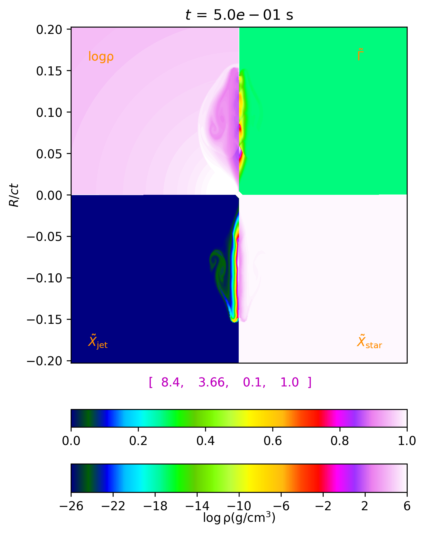 Figure 1
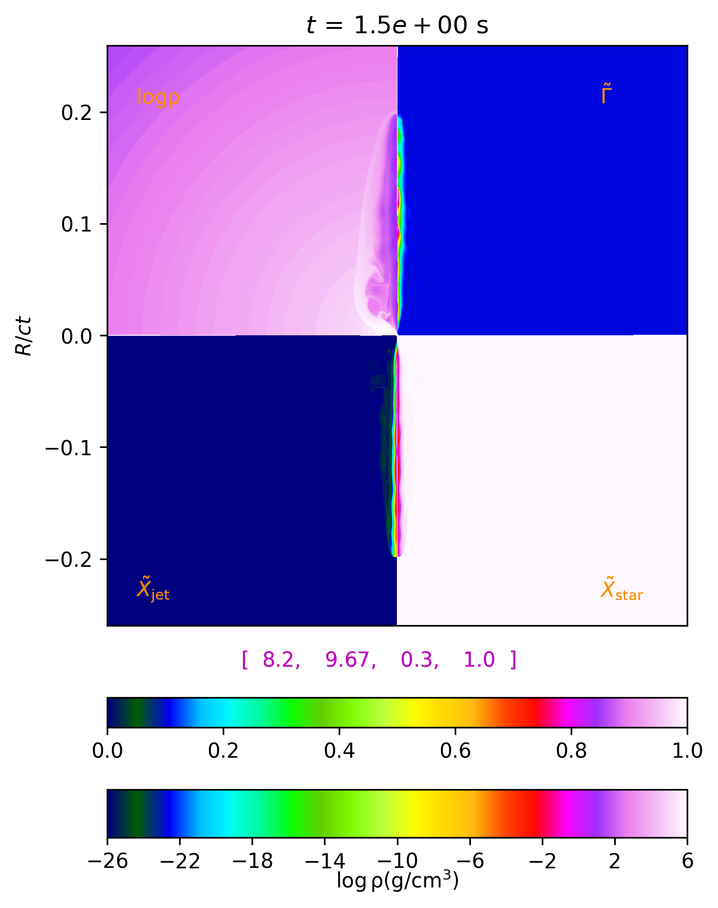 Figure 2
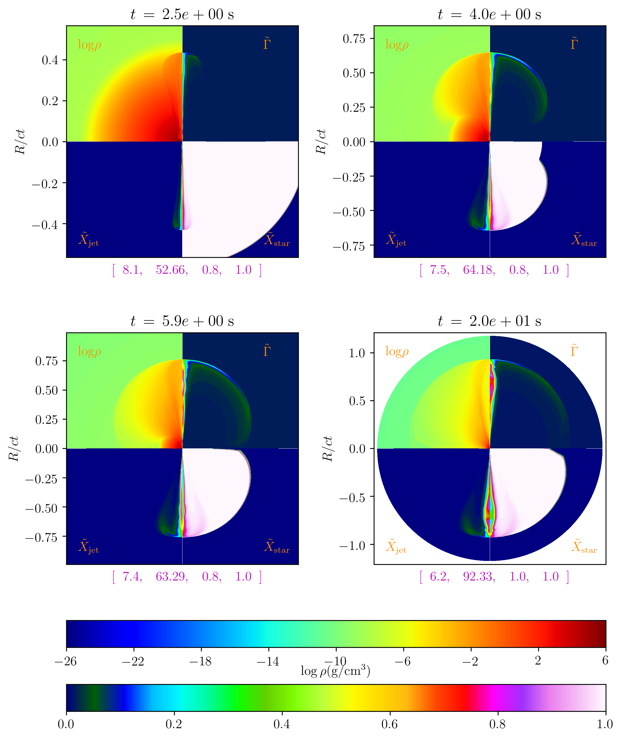 Figure 3
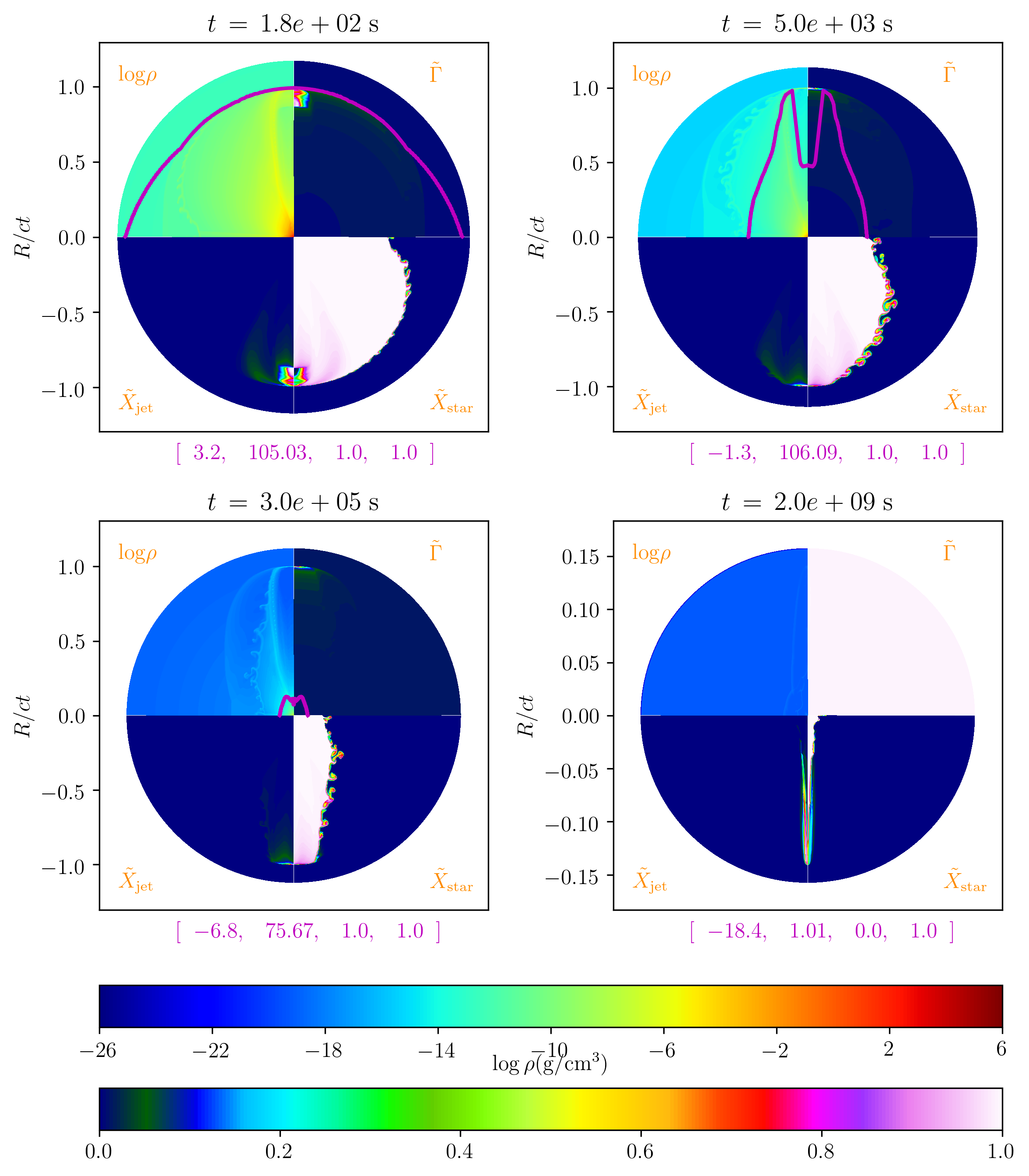 Figure 4
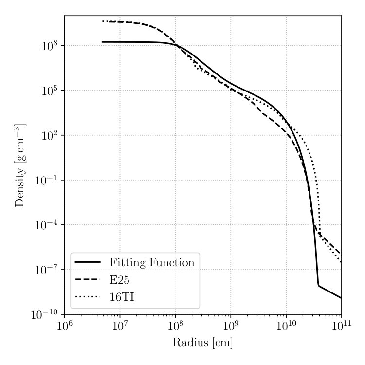 Figure 5
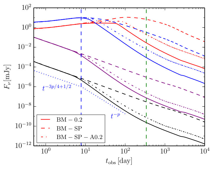 Figure 6
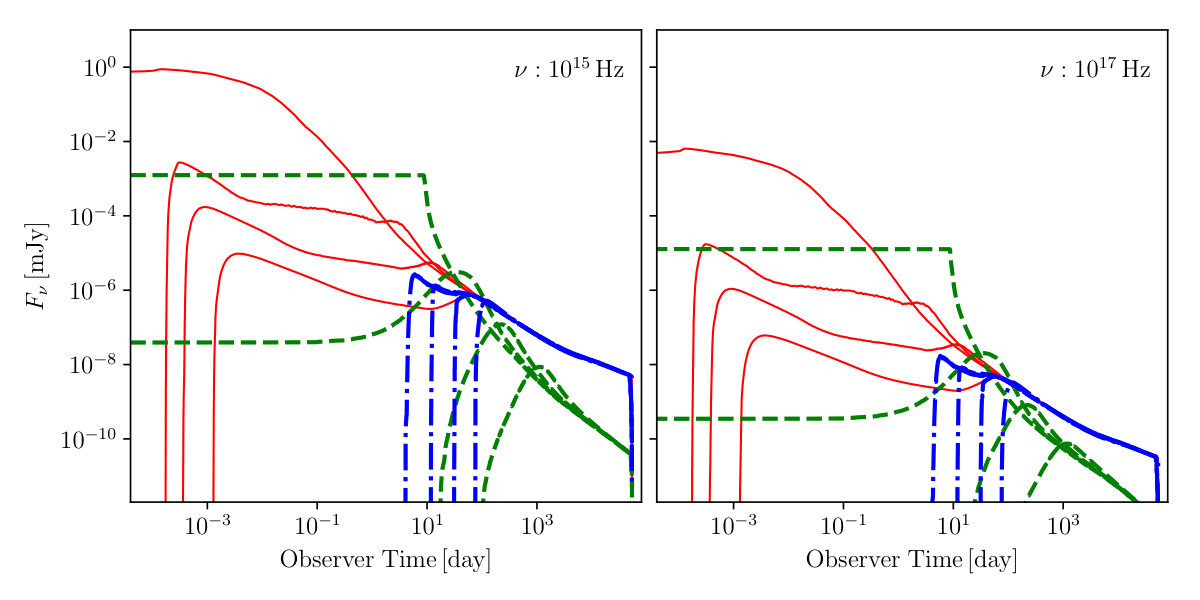 Figure 7
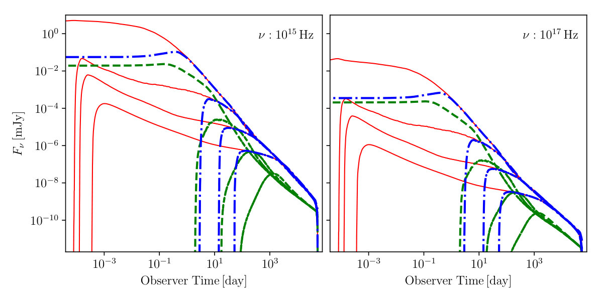 Figure 8
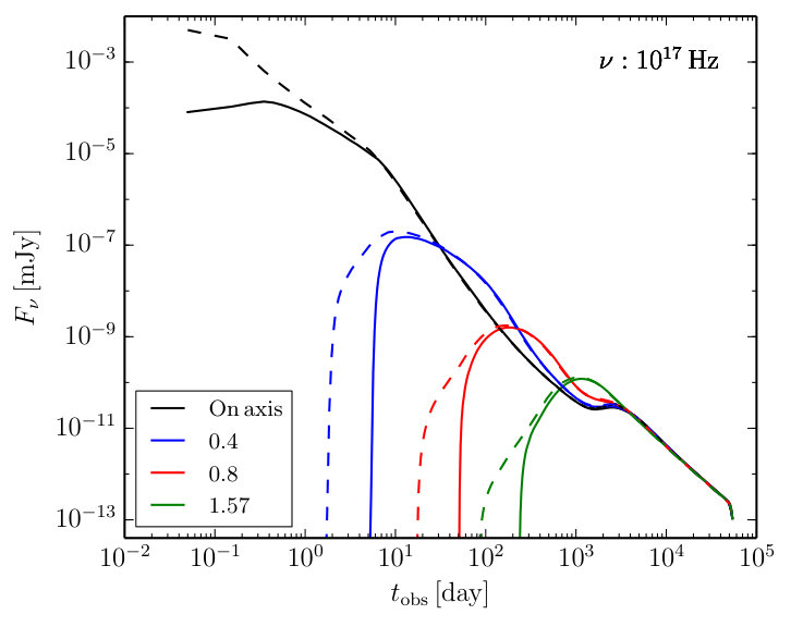 Figure 9
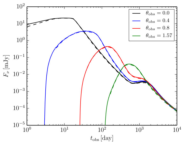 Figure 10
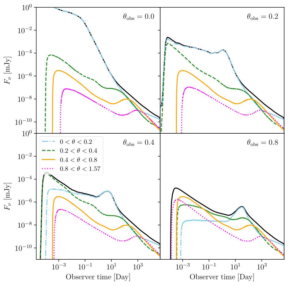 Figure 11
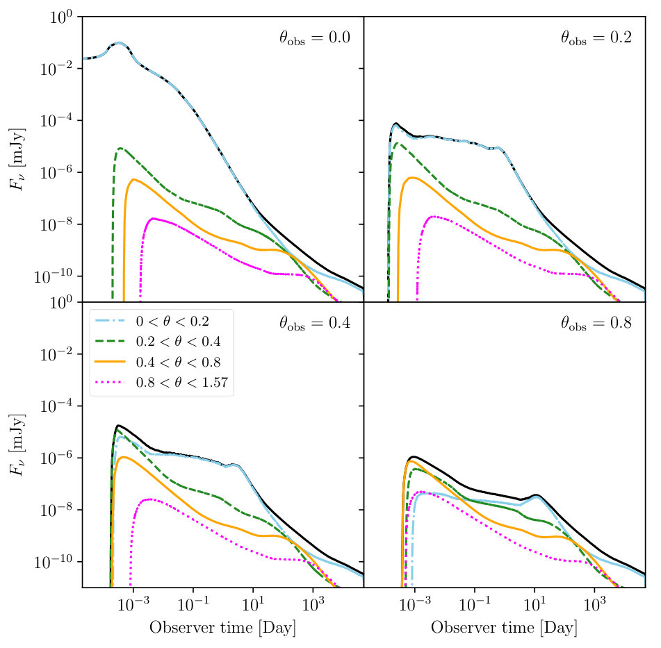 Figure 12
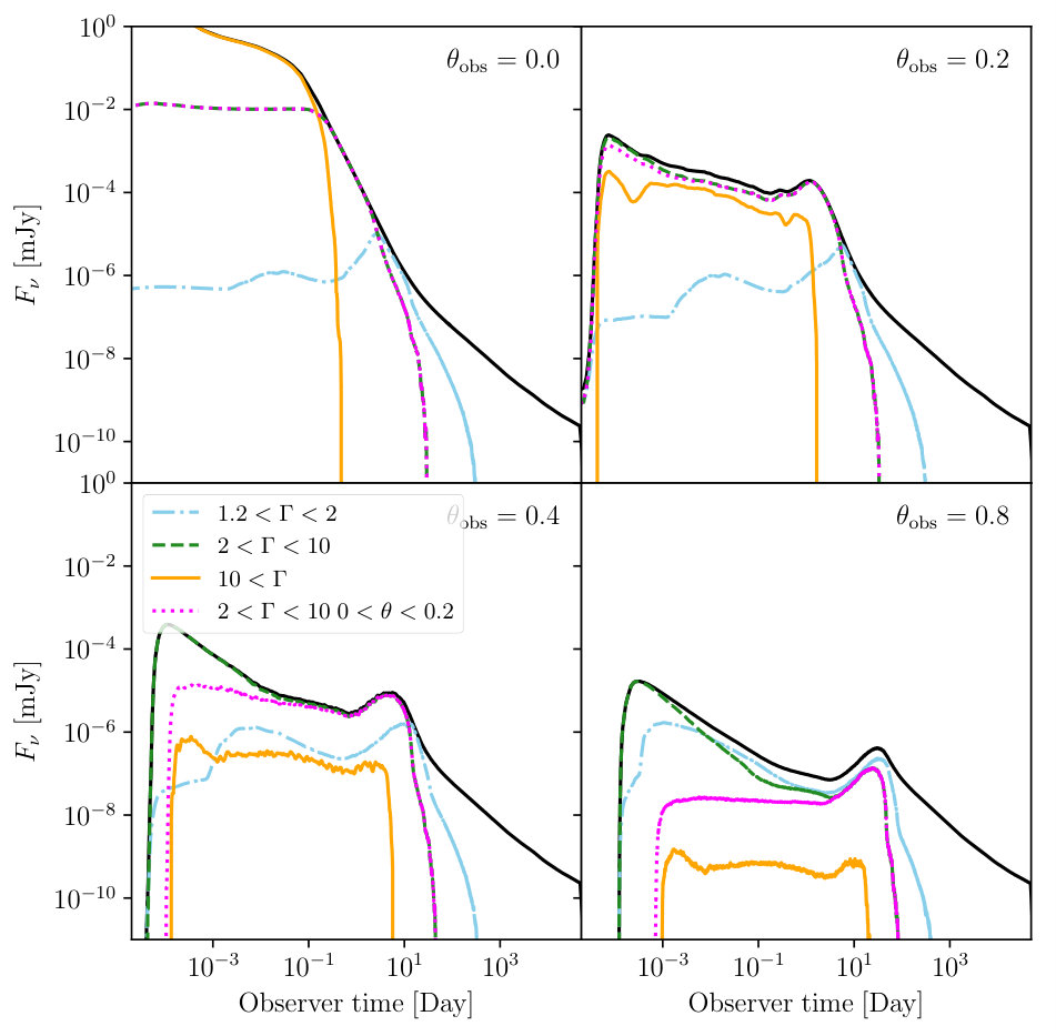 Figure 13
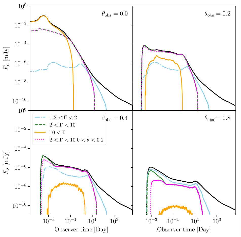 Figure 14
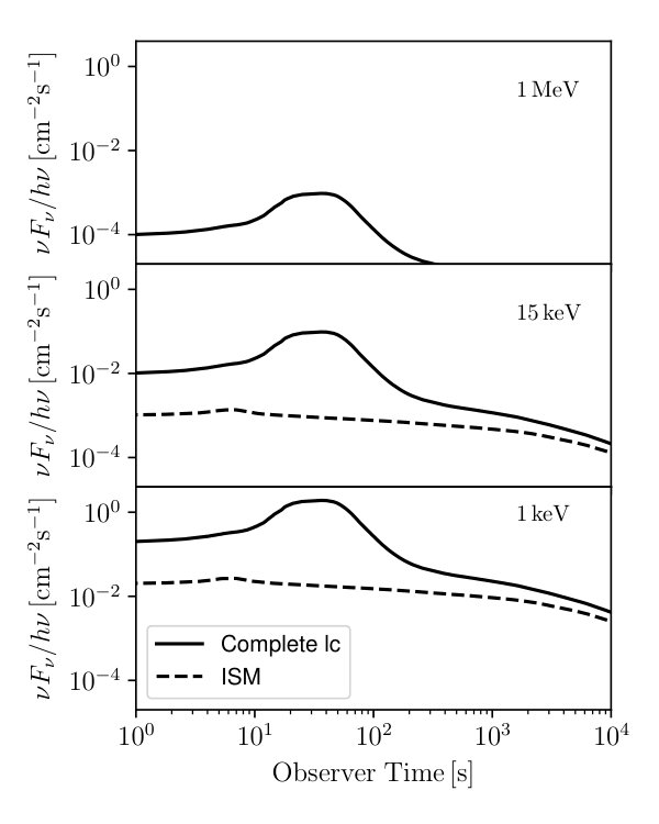 Figure 15
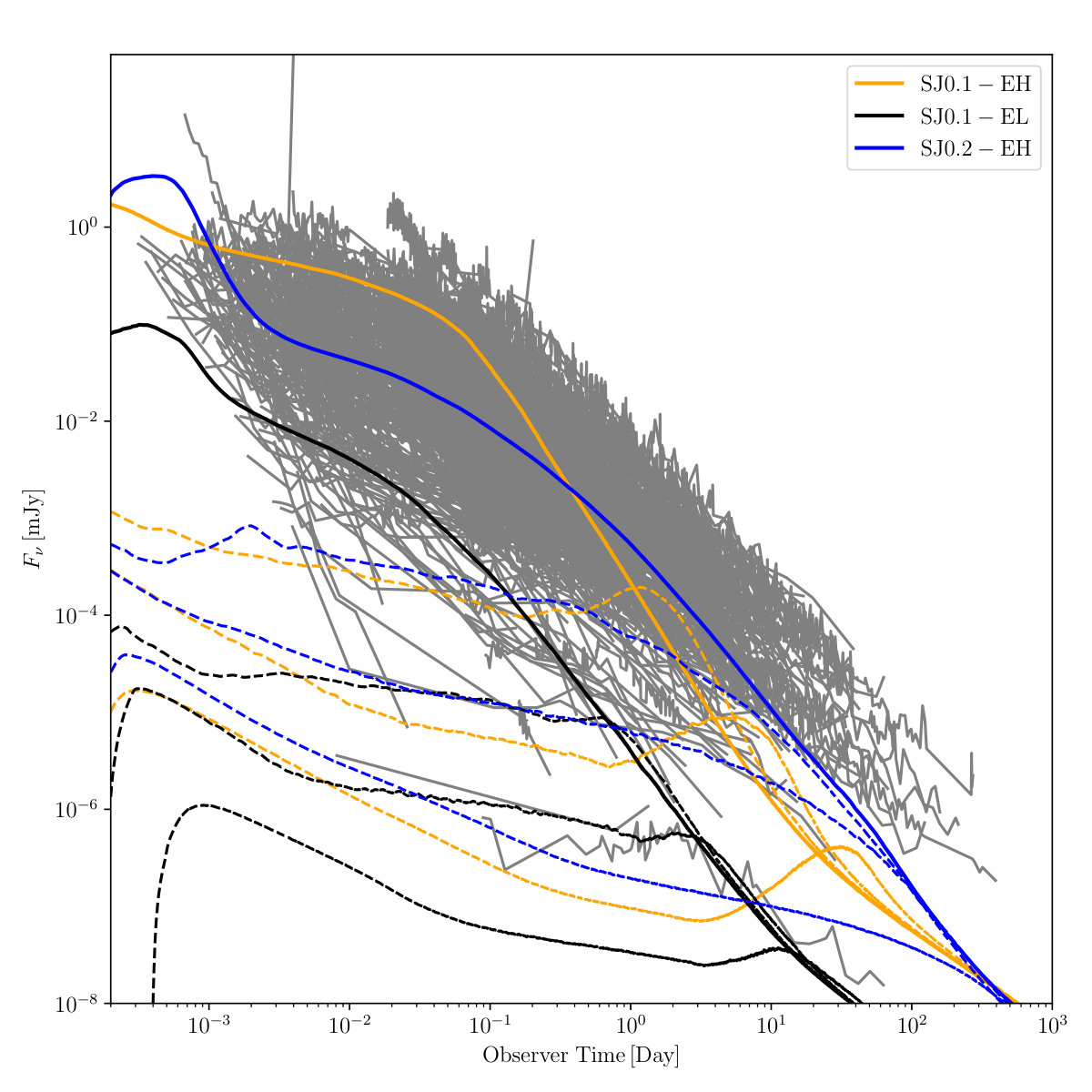 Figure 16
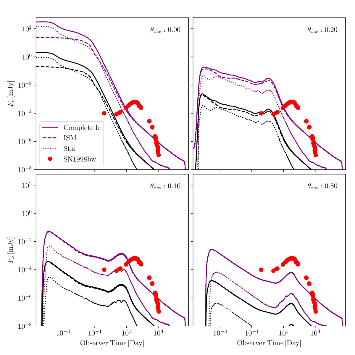 Figure 17
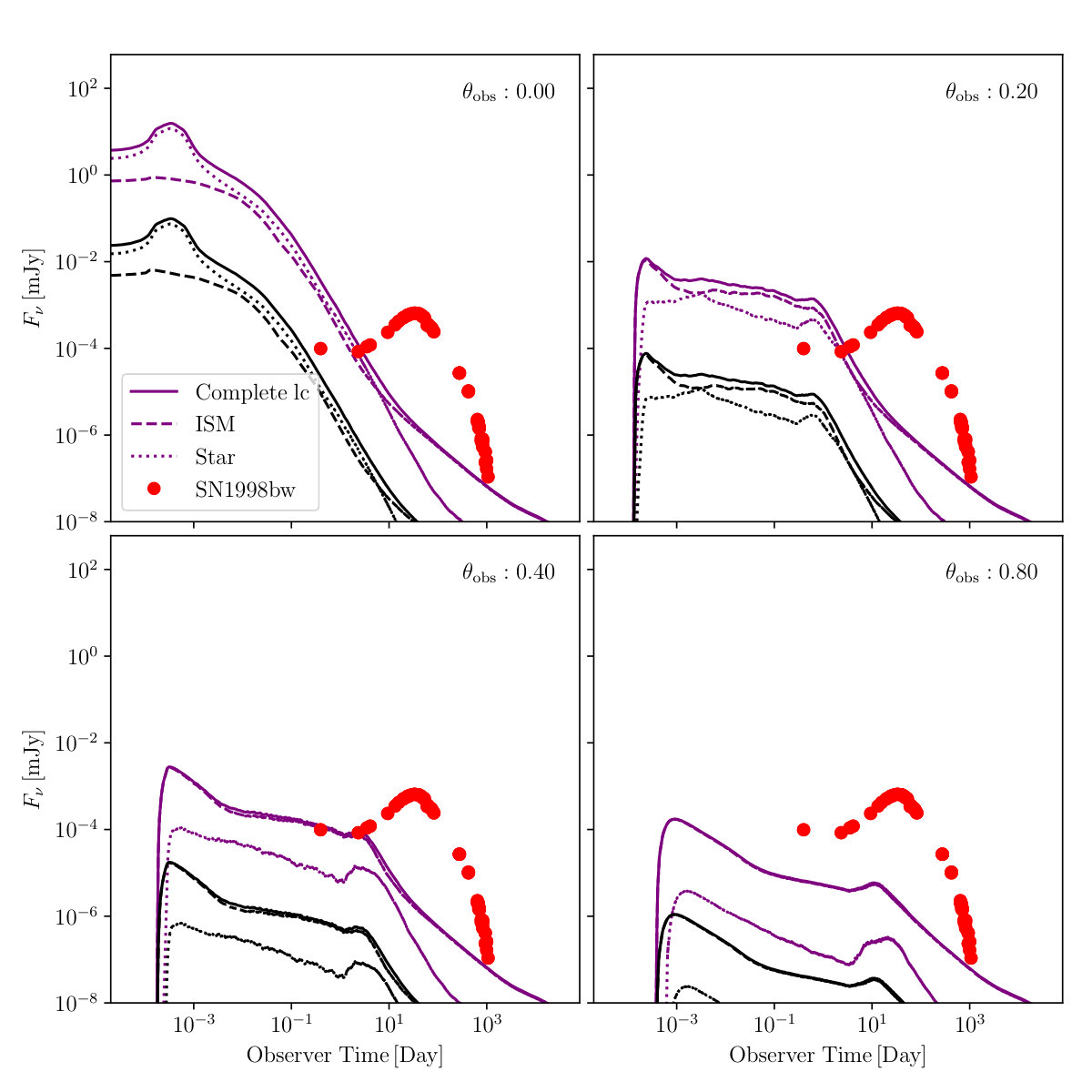 Figure 18
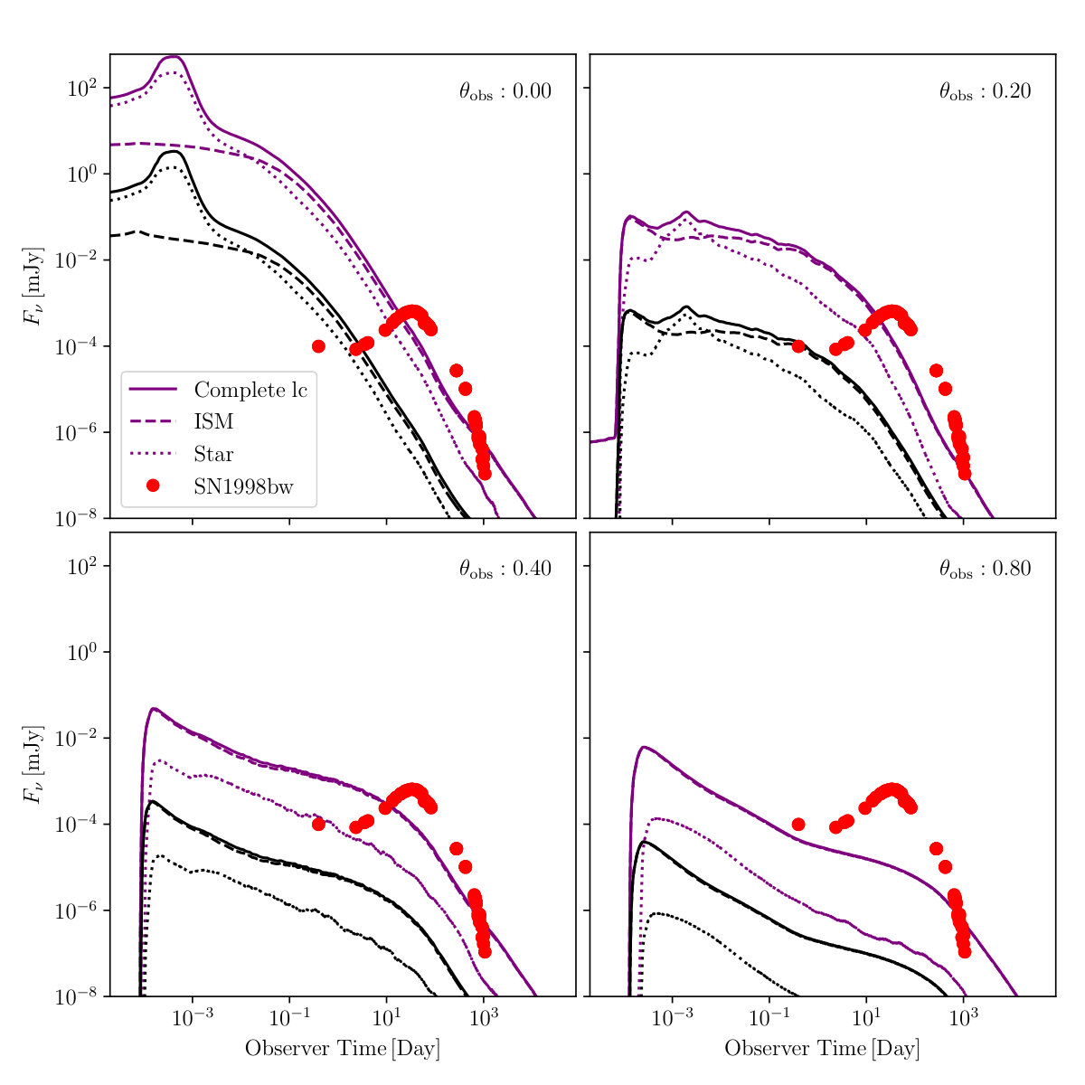 Figure 19
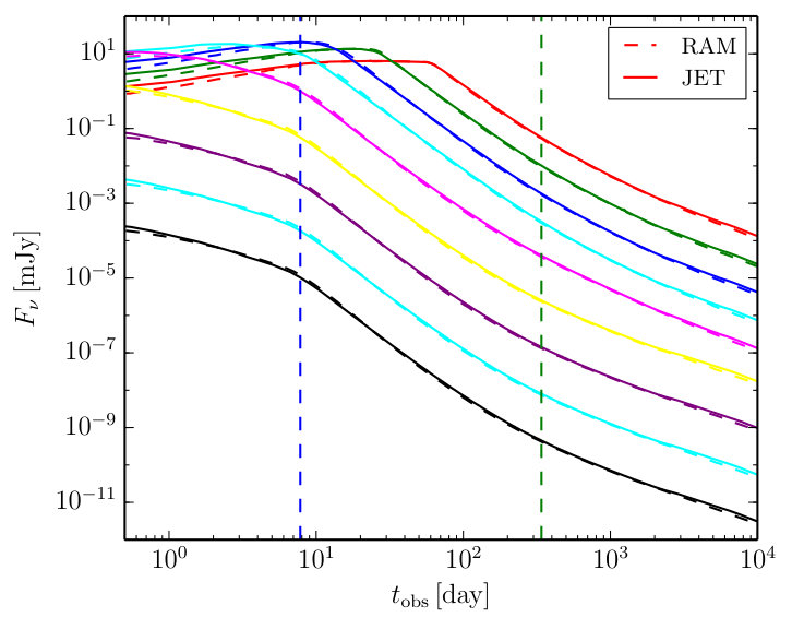 Figure 20
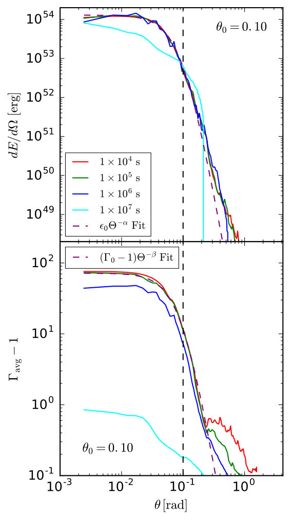 Figure 21
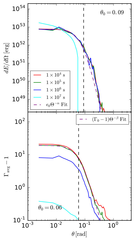 Figure 22
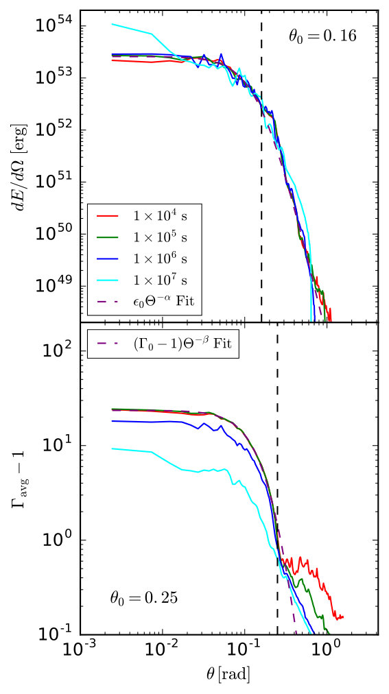 Figure 23
| Variable | BM models | Structured Jet (SJ) models |
|---|---|---|
| cm | cm | |
| Variable | Definition | Value |
|---|---|---|
| Characteristic Mass Scale | ||
| Characteristic Length Scale | ||
| Central Density | ||
| First Break Radius | 0.0017 | |
| Second Break Radius | 0.0125 | |
| Outer Radius | 0.65 | |
| First Break Slope | ||
| Second Break Slope | ||
| Atmosphere Cutoff Slope | ||
| Wind Density |
| Variable | SJ0.1-EH | SJ0.1-EL | SJ0.2-EH |
|---|---|---|---|
| 100 | 100 | 100 | |
| 50 | 50 | 50 | |
| Variable | SJ0.1-EH | SJ0.1-EL | SJ0.2-EH |
|---|---|---|---|
| 0.1 | 0.09 | 0.16 | |
| 8.9 | 7.0 | 6.7 | |
| 73 | 20 | 25 | |
| 5.1 | 3.1 | 7.9 |
Peer Reviews
No public reviews on file for this paper yet. If you reviewed it on a platform where reviews are public (OpenReview, ICLR, NeurIPS, ICML), you can paste yours below so the community can read it here.
Videos
No videos yet. Explain this paper in a talk, walkthrough, or lecture? Add one.
Off-Axis Synchrotron Light Curves from Full-Time-Domain Moving-Mesh Simulations of Jets from Massive Stars
Center for Cosmology and Particle Physics, Physics Department, New York University, 726 Broadway, New York, NY 10003, USA
Mathematical Sciences and STAG Research Centre, University of Southampton, Southampton SO17 1BJ, United Kingdom
Center for Cosmology and Particle Physics, Physics Department, New York University, 726 Broadway, New York, NY 10003, USA
Abstract
We present full-time-domain, moving-mesh, relativistic hydrodynamic simulations of jets launched from the center of a massive progenitor star and compute the resulting synchrotron light curves for observers at a range of viewing angles. We follow jet evolution from ignition inside the stellar center, propagation in the stellar envelope and breakout from the stellar surface, then through the coasting and deceleration phases. The jet compresses into a thin shell, sweeps up the circumstellar medium, and eventually enters the Newtonian phase. The jets naturally develop angular and radial structure due to hydro-dynamical interaction with surrounding gas. The calculated synchrotron light curves cover the observed temporal range of prompt to late afterglow phases of long gamma-ray bursts (LGRBs). The on-axis light curves exhibit an early emission pulse originating in shock-heated stellar material, followed by a shallow decay and a later steeper decay. The off-axis light curves rise earlier than previously expected for top-hat jet models – on a time scale of seconds to minutes after jet breakout, and decay afterwards. Sometimes the off-axis light curves have later re-brightening components that can be contemporaneous with SNe Ic-bl emission. Our calculations may shed light on the structure of GRB outflows in the afterglow stage. The off-axis light curves from full-time-domain simulations advocate new light curve templates for the search of off-axis/orphan afterglows.
Gamma-Ray Burst — Relativistic Hydrodynamic — Synchrotron Radiation— High Energy Astrophysics
††software: JET (Duffell & MacFadyen, 2013)
1 Introduction
Gamma-ray bursts (GRBs) are extremely energetic astrophysical phenomena that emit bright multi-channel transient radiation. Long duration GRBs (LGRBs) are found to be associated with type Ib/c supernova explosions (See e.g. Woosley & Bloom 2006; Modjaz 2011; Hjorth & Bloom 2012; Cano et al. 2017 for recent reviews). The observations of GRBs have long revealed two distinct phases, a prompt emission phase followed by a long-duration afterglow phase. A longstanding physical model for GRBs is the fireball model, in which the prompt -ray emission comes from internal dissipation, and the broadband afterglow is produced by external shocks with the surrounding medium (See Piran 1999, 2004; Mészáros 2006; Kumar & Zhang 2015 for reviews). Many GRB models consider the dynamics and radiation from a “top-hat jet” : a uniform outflow with a well-defined sharp edge (e.g. Rhoads 1997; Panaitescu & Mészáros 1999; Sari et al. 1999; Kumar & Panaitescu 2000; Moderski et al. 2000; Granot et al. 2001). Analytic studies and hydro dynamical simulations utilizing top-hat jet models can reproduce the achromatic break observed in the afterglow light curves of GRBs – the so called “jet break” (e.g. Harrison et al. 1999; Stanek et al. 1999). The typical explanation for the jet break is that when the relativistic jet decelerates, the observer starts to see the edge of the relativistic jet (Rhoads, 1997, 1999; Sari et al., 1999).
A natural prediction of the off-axis light curves calculated from top-hat jet models is the existence of orphan afterglows (OAs). The prompt GRB emission is strongly suppressed for off-axis observers due to relativistic beaming. However afterglow emission can be observed by off-axis observers when the inverse lorentz factor of the emitting material is less than the angle to the observer. Off-axis light curve templates inferred from top-hat jet models have been utilized to calculate the detection rate of OAs in X-ray, Optical, and radio surveys (e.g. Totani & Panaitescu 2002; Nakar et al. 2002; Zou et al. 2007; Ghirlanda et al. 2015). As of yet, OAs with light curves predicted from top-hat jets have not been definitely detected.
It is natural, however, to expect the angular profile of jet energy to decrease away from the jet axis as found in numerical simulations (MacFadyen & Woosley, 1999; MacFadyen et al., 2001; Aloy et al., 2000; Zhang et al., 2003). Various analytic jet angular structures have been proposed in the literature (Mészáros et al., 1998; Rossi et al., 2002; Zhang & Mészáros, 2002a; Kumar & Granot, 2003; Granot & Kumar, 2003), including the universal structured jet model where , and the Gaussian jet model , where is a characteristic angular scale.
Relativistic hydrodynamic simulations of GRB jets using a variety of initial conditions have been presented in the literature to model the prompt emission phase (e.g. Lazzati et al. 2009, 2011; Mizuta et al. 2011; López-Cámara et al. 2013; De Colle et al. 2018b) and the afterglow phase (e.g. Granot et al. 2001; Zhang & MacFadyen 2009; van Eerten et al. 2010; De Colle et al. 2012b, 2018a; Granot et al. 2018) separately. Duffell & MacFadyen (2015) used the moving-mesh code – JET (Duffell & MacFadyen, 2013) in two-dimensional spherical coordinates to follow the jet from deep inside the star all the way into the afterglow phase, and calculated synchrotron light curves for on-axis observers. In this work, we present similar full-time-domain (FTD) numerical simulations that cover the life-cycle of jets from deep inside the star all the way to the Newtonian phase, and calculate light curves for observers at a range of off-axis viewing angles. Collisions between the injected jet material and the stellar envelope results the formation of an ultra-relativistic outflow (i.e. the jet). We locate the photospheric position as the simulations evolve in time and calculate synchrotron radiation from the optically thin regions of the outflow. The resulting light curves cover very early phases of synchrotron emission from jet expansion. There is an initial pulsed emission for on-axis light curves which mainly comes from shocked stellar material. This may shed light on the emitting source of observed long, smooth, and single-pulsed GRBs (see Burgess et al. 2016; Huang et al. 2018 for examples). The off-axis light curve rises very early on which differs from the late rise-ups found for top-hat Blandford-Mckee (BM) jet models. In Section 2, we demonstrate the numerical improvements utilized in the simulations. We have incorporated an effective adaptive mesh refinement (AMR) scheme into the moving-mesh code - JET (Duffell & MacFadyen, 2013). We compare the AMR-enhanced moving-mesh code and the Eulerian AMR code – RAM in Section 3. In this section, we also discuss the classical top-hat BM hydrodynamic simulations and the associated afterglow light curves. In Section 4, we present the FTD dynamical evolution of jets breaking out of a stellar progenitor and discuss the emerged jet structure. In Section 5, we present on- and off-axis synchrotron light curves directly calculated from our simulations. Implications from these light curve features are made. We conclude our findings in Section 6.
2 Numerical Method
The simulations are performed with a 2D spherical axi-symmetric relativistic hydrodynamic (RHD) moving-mesh code– JET (Duffell & MacFadyen, 2013). The code numerically integrates the following equations:
[TABLE]
where is proper density, is enthalpy density, is pressure, is internal energy density, and is the four-velocity, where the speed of light is set to one. The equations are solved in two dimensional spherical coordinates assuming axisymmetry. The source terms and are used to model the injection of mass, momentum, and energy on small scales by the central engine. We employ RC equation of state (EOS) in our simulations which matches the exact Synge equation within an accuracy of (Ryu et al., 2006). We express the specific enthalpy as a function of . and utilize Newton-Raphson iteration to find the root of based on the values of conservative variables. The new primitive variables are then calculated accordingly. Detailed procedures are covered in De Colle et al. 2012a. Different EOS could be adopted in simulations by changing the expression of . Equation 3 - 5 corresponds to the specific enthalpy function subject to ID (ideal gas law) EOS, TM EOS (Mignone et al., 2005), and RC EOS (Ryu et al., 2006), respectively:
[TABLE]
We use the HLLC Riemann solver (Mignone & Bodo, 2005) and move the radial numerical cell faces at the local contact discontinuity (CD) velocity. In the vicinity of the shock front, high resolution along the radial direction is required to fully resolve the dynamics of the relativistic structures in the outflow. The AMR scheme, which actively refine cells in the relativistic region and derefine cells within non-relativistic gas, are implemented within Eulerian RHD code frame (e.g. Fryxell et al. 2000; Zhang & MacFadyen 2006; De Colle et al. 2012a). The time step size is, however, limited by the finest cells with high velocity. The moving-mesh technique, with each cell moving at approximate the local CD velocity, can enlarge the time step (see e.g. Duffell & MacFadyen 2011, 2013). The combination of these two techniques in principle allows accurate simulations of relativistic jets in efficiency. In this work, we incorporate a robust AMR scheme into the moving-mesh code. We define an approximate numerical second derivative of fluid variables as a measurement of error:
[TABLE]
which is utilized in empirical AMR schemes (see e.g. Fryxell et al. 2000; Zhang & MacFadyen 2006). By default, we set the adjustable parameter in the denominator to 0.01. The spherical domain is evenly distributed in the angular direction with radial tracks, yielding an angular resolution of . The radial tracks shear with the radial velocity of the gas. Each radial track moves independently, behaving essentially as 1D Lagrangian grid (Duffell & MacFadyen, 2013). In each time step, the cell along a radial track with the maximum measurement of error will be refined if . The cells with will be considered to be derefined. The final choice of the cell to be derefined, for each radial track, is the one that has the smallest time step. The time step of each cell is estimated according to the CFL condition , where is a constant, is the radial cell length, is the characteristic wave speed calculated at the cell face, is the radial velocity of the cell face (i.e. the local CD velocity). Initially, the spherical domain is logarithmically spaced in the radial direction, and the aspect ratio of each cell is of order one. For relativistic explosions, the dynamical scale: sets the desired radial resolution of the relativistic shell. This gives us an estimation of the required aspect ratio in order to resolve the relativistic shell: . This criteria has been incorporated into the AMR scheme to determine whether or not to derefine the high-resolution cells in the ultra-relativistic region. With cell faces moving radially at the local CD velocity, the aspect ratio of each cell is adjusting dynamically. The simulations performed in this study have maximum Lorentz factor around . The maximum dynamic aspect ratio reaches about 450. Also, we find the combined scheme is able to accurately simulate an ultra-thin relativistic jet with a Lorentz factor up to . Compared with the traditional Eulerian AMR scheme, the AMR-enhanced moving-mesh scheme delivers accuracy in efficiency.
3 Top-hat Blandford-McKee Models
3.1 Code comparison
We perform standard top-hat Blandford-Mckee (BM) (Blandford & McKee, 1976) simulations to check the robustness of the new AMR-enhanced moving-mesh scheme. For the BM solution, the Lorentz factor of the shock front , the Lorentz factor of the fluid , the elapsed time , and the jet radius follow the relations (the speed of light is set to one):
[TABLE]
The half opening angle of the top-hat BM jet () is set to . The isotropic equivalent energy is . The uniform ambient density is set to 1 proton per cubic centimeter, and the pressure is set to following previous Eulerian AMR simulations (Zhang & MacFadyen, 2009; van Eerten et al., 2010). The hydrodynamic simulation starts at the moment when the initial Lorentz factor of the fluid just behind the shock is . In Figure 1, we demonstrate that the on-axis synchrotron light curves calculated from our BM simulation match well with results (as presented in Zhang & MacFadyen 2009) from simulations performed with the Eulerian AMR code - RAM (Zhang & MacFadyen, 2006). We calculate the broadband synchrotron radiation light curves utilizing a well-tested synchrotron radiation code (Zhang & MacFadyen 2009; van Eerten et al. 2010, see also Sari et al. 1998; De Colle et al. 2012a). The same radiation parameter values are used in both calculations: the electron equipartition factor , the magnetic equipartition factor , and the energy power-law index of relativistic electron . The flux distance scaling is set to as in Zhang & MacFadyen (2009). We also adopt the same EOS (TM-EOS) in this simulation for a fair comparison.
For off-axis light curves, we compare with results from van Eerten et al. (2010). As shown in Figure 2, off-axis light curves from our BM simulation (solid lines) match well with results from van Eerten et al. (2010). One advantage of our new scheme is that we’re able to perform accurate top-hat BM simulations at an earlier time with Lorentz factor of hundreds instead of tens.
Observational results indicate that GRB afterglow comes from ultra-relativistic jets with inferred Lorentz factor . Numerical simulations with initial Lorentz factor are thus necessary to fully capture early afterglow emission. Here, we perform two top-hat BM simulations with different initial Lorentz factors: (1) (denoted as BM-J0.2-G100 simulation). (2) (denoted as BM-J0.2-G20 simulation), respectively. The RC-EOS is adopted for both BM simulations (hereafter, all the simulations are performed with RC-EOS). The synchrotron radiation parameter values are listed in Table 1. The on- and off-axis synchrotron light curves at frequency from the BM-J0.2-G20 simulation and from the BM-J0.2-G100 simulation are over-plotted in Figure 3. The early on-axis light curve calculated from BM-J0.2-G100 simulation (dashed line) is an order of magnitude larger than that from the BM-J0.2-G20 simulation. The off-axis light curves from the BM-J0.2-G100 simulation rise up earlier. At a later time, the afterglow light curves from both simulations overlap with each other.
3.2 Characteristics of on- and off-axis top-hat BM light curves
The top-hat jet model can explain the “jet break” phenomena observed in GRB afterglows. On-axis observers will start to see the edge of the jet when its Lorentz factor drops to . The missing flux will lead to a break in the slope of observed light curves. Before the jet break time, the temporal slope of high frequency light curves () scales as . This should be the same for both spherical explosion and top-hat jets. After that, the light curve of the finite top-hat jet scales as (see e.g. Rhoads 1999; Sari et al. 1999).
We perform a spherical BM simulation with parameters identical to the BM-J0.2-G100 model. The light curves from the spherical BM simulation (see dashed lines in Figure 4) do not show any break. When we cut a conical segment with half opening angle , and only add emission from this region, the calculated light curves (dotted-dashed line) display the expected temporal break due to pure relativistic beaming. For the light curve of top-hat BM-J0.2-G100 simulation (Solid line), the jet break happens at around the same time but with a steeper temporal slope. The extra decay then originates from a well-know hydrodynamic effect: lateral spreading of the jet (Rhoads, 1999; Sari et al., 1999; Granot et al., 2001; Zhang & MacFadyen, 2009; Wygoda et al., 2011; van Eerten & MacFadyen, 2012; Granot & Piran, 2012; Duffell & Laskar, 2018). The comparison among these three sets of light curves indicates that the jet break phenomenon due to hydro-dynamical effect is not negligible even for the relatively simplified model considered here.
For off-axis light curves, a natural prediction from top-hat jet models is the existence of “orphan” afterglows. An observer located outside of the opening angle of relativistic jets will not be able to detect the early high energy emission due to relativistic beaming. At a later time when the Lorentz factor of the jets reduces to , the off-axis observer starts to receive emission from the central jet at lower energies. It is then possible to detect the afterglow radiation without having detected prompt emission for off-axis observers. As shown in Figure 2, the off-axis afterglow emission show features of late rise-up, on a time scale of days to months depending on the viewing angle. However, as we show in Figure 3, changing the initial Lorentz factor from 20 to 100 leads to an early rise-up for off-axis light curves. The explanation is that the BM-J0.2-G100 profile is set at an earlier time , and at a smaller radius .
In the rest of the paper, we utilize FTD simulations to study the on- and off-axis synchrotron light curves of LGRB jets. We discuss features revealed from the light curves and their implications.
4 Full-Time-Domain Jet Simulation
4.1 Initial numerical setup
The stellar progenitor before collapse utilized in the simulations follows the analytical model in Duffell & MacFadyen 2015. This model approximates the output of a MESA (Paxton et al., 2011, 2013) simulation where a low-metallicity rapidly rotating star evolves to a Wolf-Rayet star. The density as a function of radius is:
[TABLE]
The parameters in the above Equation are listed in Table 1 of Duffell & MacFadyen (2015) and are included here for clarity (see Table 2). The velocity and pressure are initially set to negligible values. Self-gravity and stellar rotation are not included in the simulations.
The jet engine is initiated at around the radius using a source term. From this distance, the density field of the progenitor in which the jet propagates is comparable to that of the E25 model in Heger et al. 2000 and the 16TI model in Woosley & Heger 2006 (see Figure 5). The jet engine model utilizes the nozzle function in Duffell & MacFadyen (2015). For clarity, the expressions are included in the following:
[TABLE]
where is the normalization of via the integration over :
[TABLE]
The source terms in Equations (1) and (2) are given in the following:
[TABLE]
This jet engine features a smoothly decaying tail with an average engine duration . The engine completely shuts down at around (see discussions of engine duration in e.g. Lazzati et al. 2013). The simulation (denoted as SJ0.1-EH (Energy High) hereafter) performed in this study differs from Duffell & MacFadyen 2015 in two ways. First, we utilize the incorporated AMR scheme which enforces the criteria to better resolve the relativistic shell. Second, we adopt the newly implemented RC-EOS instead of the original ideal gas EOS. We also perform additional simulations. One with relatively low jet engine energy (denoted as SJ0.1-EL). Another with a different jet engine half opening angle (denoted as SJ0.2-EH). The jet engine parameter values for these three models are listed in Table 3.
To better interpret the role of each fluid component, we use three passive scalars to track the mass fraction of each individual component filling the cells. The subscript labels each individual component: 1 for stellar progenitor, 2 for ISM material, and 3 for jet engine material. Initially, is set to inside the progenitor and in the ISM. Three auxiliary equations are solved accordingly (Duffell & MacFadyen, 2013):
[TABLE]
The conserved mass for each component () is updated based on the density flux through the cell boundary and the addition of source term (for the injection of jet engine material). Dividing the individual conserved mass by the total conserved mass () gives us the new primitive passive scalar .
4.2 Dynamical details of the full-time-domain jet simulation
4.2.1 launch of jet engine
Figure 6 shows the early evolution of jet engine flow upon injection. The ram pressure generates a bow shock. Dense stellar material gets pushed to the side, forming a cocoon which confines the engine outflow. A high-density wedge of stellar material develops at the head of the jet. It shreds jet engine materials from the head. These engine materials curl back, forming vortexes. These vortexes then detach from the jet and get swept backward relative to jet propagation. This vortex shedding phenomena is, generally speaking, similar to that found in previous simulations (Scheck et al., 2002; Mizuta et al., 2004; Morsony et al., 2007). The speed of jet head keeps increasing, soon exceeds the local sound speed (At the time , the Lorentz factor of the head of jet is as shown in Figure 6). The backflow becomes quasi-straight to the main jet (Mizuta et al., 2010). At early times, the bow shock has a narrow head and a wide tail. When it approaches the surface, the jet head expands in the low density envelope as shown in the next subsection (see also e.g. Zhang et al. 2003, 2004b). We use spherical coordinate to conduct simulations. As jets propagate outward, the width of the cell increases. Features of the inner part of jet (close to pole) may not be fully resolved. We well resolve the relativistic shell in the radial direction via previously described AMR scheme. As the ultra-relativistic jet shell penetrates the progenitor, the stellar material that lies on top of the jet easily gets pushed aside. No strong “plug” instability has been seen (Lazzati et al., 2010; Mizuta & Ioka, 2013; Gottlieb et al., 2018a; Xie et al., 2018).
4.2.2 propagation of the jet
Figures 7 and 8 show snapshots of the simulation domain at different stages of jet evolution for the SJ0.1-EH model. Each snapshot displays the contour of log density, normalized Lorentz factor, and normalized mass fraction of jet engine/stellar material. At lab frame time , the jet outflow begins to expand in the low-density wind. The shock wraps around the star as shown in the snapshots at and . At a later time, , the shock accelerates and approaches its terminal Lorentz factor . The engine completely turns off at around this time. Along the polar axis, a relativistic blob forms behind the shock front. Through internal collisions, the relativistic blob forms an ultra-relativistic thin shell. At first, the relativistic shell is hidden behind the photosphere (indicated by the magenta line in Figure 8). We define the photosphere as the place where the optical depth is unity. We estimate the optical depth according to:
[TABLE]
where is the Thomson scattering cross section, is the absolute value of the velocity normalized by speed of light, is the Lorentz factor of the gas, is the angle between the velocity vector and the line of sight, is the electron number density (Abramowicz et al., 1991; Mizuta et al., 2011). In detail, we first initiate sufficient number of tracing rays at the given observing angle. Each tracing ray will enter the spherical domain from a position of the outer boundary. We then calculate the crossed length in each cell the ray intercepts and perform the integration of optical depth (Equation 17), assuming the density is uniform within the cell. The contribution of optical depth from materials outside of the simulation domain is added using an analytical expression. Following this procedure, we’re able to get the optical depth for all of the cells in the simulation domain at each snapshot. Note that, this procedure is a simplified version in terms of the calculation of actual photosphere. Photons are propagating in a turbulent, evolving density background. Integration of optical depth over continous snapshots is then preferred. In this work, we focus on the study of optically-thin synchrotron radiation light curves. Once the emitting shell breaks out of the photosphere, the photosphere position has no impact on the shape of the light curve. We find the characteristics of synchrotron light curves are not sensitive to the exact definition of photosphere. For detailed treatment of photons breaking out of the photosphere, we refer readers to the study of photospheric emission (e.g. Mizuta et al. 2011; Lazzati et al. 2011; De Colle et al. 2018b; Gottlieb et al. 2018b).
A wind profile is adopted here to describe the density field of surrounding interstellar medium (ISM): . The photosphere is initially located at a radius . At around , the shock front breaks through the original photosphere. The photosphere then advances outward with the jet. Eventually, at around , the photosphere begins to fall behind the relativistic shell. The process of jet breaking out of the photosphere covers the dynamical distance where prompt emission is estimated to occur (e.g. Piran 1999; Kumar & Zhang 2015). At , the photosphere falls far behind the relativistic shell, and Kelvin-Helmholtz instability is seen behind the shock front. At , the jet reaches a distance . At this time, the jet and stellar material forms a highly aspherical structure and has become fully Newtonian.
4.3 Angular structure of the jets
The angular structure of the jets features an ultra-relativistic core, primarily composed of jet-engine material. The core is surrounded by a mildly relativistic sheath (see Figure 8). The angular distribution of the total energy (excluding rest mass energy) , and energy-averaged Lorentz factor for the emerged jet, are shown in Figure 9. During the coasting period s, the jet angular structure does not change significantly. They can be well fit by a universal structured jet (USJ) model in which and varies as a power law of polar angle (Kumar & Granot, 2003; Granot & Kumar, 2003; Granot & van der Horst, 2014),
[TABLE]
where are free fitting parameters. We fit the three performed simulations: SJ0.1-EH, SJ0.1-EL, and SJ0.2-EH, and list their fitting parameter values in Table 4. As shown in Figure 9, the half opening angle of the central core is for the SJ0.1-EH and SJ0.1-EL simulations, and for the SJ0.2-EH simulation. The total energy of the jet core: for SJ0.1-EH and SJ0.2-EH, and for SJ0.1-EL, falls within the inferred range of GRB kinetic energy (see e.g. Frail et al. 2001; Panaitescu & Kumar 2002; Berger et al. 2003a; Lloyd-Ronning & Zhang 2004; Goldstein et al. 2016). The angular power-law decay index in all of the simulations is significantly larger than , the typical value adopted in the USJ model (Rossi et al., 2002; Zhang & Mészáros, 2002a; Granot & van der Horst, 2014). An observational correlation between the isotropic emitted energy and the spectral peak energy : has been discovered (Amati et al., 2002). This relationship extends from gamma-ray bursts (GRBs) to X-ray flashes (XRFs) (see e.g. Lamb et al. 2005). In the unified GRB-XRF model, XRFs are the result of a highly collimated GRB jet viewed off axis (Yamazaki et al., 2002; Lamb et al., 2005). The observed range is more than orders of magnitude (see e.g. Zhang et al. 2004a). For the USJ model with , the relation implies that the viewing angles of XRFs need to be at least 2 orders of magnitude larger than those of GRBs. This puts strong constraint on the USJ model with (or vice-versa the unified GRB-XRF model). Zhang et al. 2004a shows that a quasi-universal Gaussian-like structured jet model with a steeper angular profile can reconcile this. The structured jets emerged in our simulations feature a steep angular profile with . This profile can also explain the wide range of observed values for given limited off-axis observer angles. We only need to have a viewing angle several times larger than to get an XRF whose is times lower than the typical GRB (Zhang et al., 2004a).
5 Synchrotron light curves from full-time-domain jet simulations
The FTD jet simulations reveal that jets emerging from the stellar progenitor have characteristic structure that differs from top-hat jet models. We expect the light curve from realistic jets will differ from top-hat jet models as well. In Figure 10, we plot multi-frequency on- and off-axis synchrotron light curves calculated from the optically thin regions of the simulation domain. The micro-physical radiation parameters are listed in Table 1. In this study, we do not consider synchrotron self-absorption and focus our attention on optical and X-ray emission. We present light curves that cover a wide range of time from the order of seconds to the order of years. For comparison, we also include the scaled R-band light curve of supernova SN1998bw (Galama et al., 1998; Guillochon et al., 2017). For a typical GRB-SN, there are two major components (1) the afterglow (AG), which is associated with the GRB event, (2) the supernova (SN). Clear SN bumps are observed for many GRB-SN events (for reviews, see e.g. Woosley & Bloom 2006; Modjaz 2011; Hjorth & Bloom 2012; Cano et al. 2017).
5.1 Implications for on-axis prompt emission
As seen in Figure 10, the on-axis light curves start with an early pulse followed by three major segments: an early time decay, a shallow decay, and a late steeper decay. These light curve components share similarities with canonical X-ray afterglows observed by the Swift X-ray Telescope (XRT) (Gehrels et al., 2009; Kumar & Zhang, 2015). The time scale of the early pulse is tens of seconds (see Figure 11 for an example), and falls within the duration of observed LGRB prompt emission. The light curve decomposition shows that the on-axis multi-frequency light curves from shock-heated ISM (dashed lines) are flat for the entire duration of prompt and shallow decay phases. We thus find the pulse mainly originates from shock-heated stellar material. Long and temporally smooth GRBs with typical variability timescales larger than a few seconds are observed and sometimes considered to arise from an external shock (Burgess et al., 2016; Huang et al., 2018).
On-axis light curves from FTD simulations provides hints that, while an unified external shock model can explain both prompt and afterglow emissions, the prompt -ray emission of observed single pulsed GRBs may still come from shock-heated stellar materials instead of freshly shock-heated ISM materials (e.g. Burgess et al. 2018). Noted that, GRB prompt emission involve more complicated physics (photospheric emission, magnetic reconnection for example). Here we simply give the implication based on the analysis of hydrodynamic results.
5.2 Implications for off-axis afterglow radiation
The off-axis light curves (seen in Figure 10) exhibit clear temporal breaks as well. The break time depends on the viewing angle. Wang et al. 2015 fit the broken power-law (BPL) model to optical and X-ray light curves of 85 GRBs, and find that the break times range from a few to after the GRB prompt emission. The break times seen in on-axis light curves in Figure 10 fall in this range. For off-axis light curves, an achromatic re-brightening component may appear around the break time and is then followed by a steeper decay. This is what happens for off-axis light curves from narrow jet simulations SJ0.1-EH and SJ0.1-EL, but not from the wider jet simulation SJ0.2-EH. Re-brightening features occur in observations of long GRBs (e.g., GRB070311 Guidorzi et al. 2007, GRB081028 Margutti et al. 2010, GRB100814A De Pasquale et al. 2015, GRB120326A Melandri et al. 2014; Hou et al. 2014 ), short GRBs (e.g., GRB050724 Campana et al. 2006, GRB080503 Gao et al. 2015), and X-ray flashes (e.g., XRF030723 Huang et al. 2004). Various mechanisms have been proposed to explain these rebrightenings. Here we list three: the density jump model (Lazzati et al., 2002; Dai & Wu, 2003; Tam et al., 2005; Uhm & Zhang, 2014; Geng et al., 2014), the refreshed-shock or energy injection model (Dai & Lu, 1998; Rees & Mészáros, 1998; Kumar & Piran, 2000; Sari & Mészáros, 2000; Zhang & Mészáros, 2001; Zhang & Mészáros, 2002b; Granot & Kumar, 2006; Zhang et al., 2006; Dall’Osso et al., 2011; Uhm et al., 2012; Laskar et al., 2015), and the two-component jet model (Berger et al., 2003b; Huang et al., 2004, 2006), Other models can be found in e.g. Kong et al. 2010. The FTD jet simulations demonstrate that structured jets can naturally drive the re-brightening afterglow component for off-axis observers. The ratio of its temporal width to its peak time is . This feature is clearly different from X-ray flares which characterize short rise time (e.g. Fan & Wei 2005; Burrows et al. 2005; Zhang et al. 2006; Liang et al. 2006). Before the re-brightening, the flux decays as segments of power-law. This early decaying component for off-axis light curves originates from the shocked ISM which is different from the rapidly fading “merger flash” – the non-thermal cooling emission of shock-heated merger ejecta and jet engine materials propagating in a low density environment. The magnitude of the early X-ray “merger flash” for GRB170817A has been estimated to lie below the instrument-detection limit of Swift when its X-ray Telescope made the first observation of the merger site (Xie et al., 2018). The comparison of the shape of off-axis light curves presented here and those in Xie et al. 2018 shows that even though structured jets are produced in both scenarios, different set-ups of ISM density and progenitor profile can drive distinct off-axis light curves. In the work of Xie et al. 2018, the late off-axis afterglow light curves keep increasing before the external shock decelerates. In this new piece of work, we adopts a dense wind ISM profile. The off-axis external shock is decelerating after breaking out of the photosphere (revealed in the decreased value of Lorentz factor in Figures 8 and 9. The off-axis light curves in this case decay with time in the beginning. The late afterglow emission (including the re-brightening components) may be overshadowed by on-going supernova emission (see Figure 10).
The long time monitoring of Type Ib/c SNe do not present evidence for a steeply rising light curve (Soderberg et al., 2006; Bietenholz et al., 2014; Ghirlanda et al., 2014; De Colle et al., 2018a). However, broad-lined Type Ibc supernovae (SNIbc-BL), including those lacking prompt GRB emission, may be producing off-axis afterglow components which, if disentangled from supernova emission, would indicate that they harbor off-axis GRBs (see e.g. Modjaz et al. 2019).
5.3 light curve decomposition
To better interprete the features of light curves from FTD simulations, we decompose the on- and off-axis light curves based on the lateral angle and Lorentz factor distribution of emitting materials in the shell (shown in Figure 12 and Figure 13). For on-axis light curves, the materials confined within a lateral angle 0.2 determines the light curve shape for the first , covering the prompt to early normal decay phases. The flattening part of late normal decay () mainly comes from high latitude emission () (see Figure 12). The first light curve, especially the early pulse, are emitted by materials with high Lorentz factor (), while the flattening part of late normal decay comes from sub-relativistic materials with (see Figure 13). For off-axis light curves, the early decay part originates from the angular region that is close to the observers’ light of sight. For example, at the off-axis viewing angle , the materials within the angular region drives the early decay. As time goes on, the emission from the central region gradually becomes important. It flattens the light curve and eventually drives the re-brightening components (see off-axis light curves from SJ0.1-EH and SJ0.1-EL simulations). After re-brightening, the off-axis light curves go through a steeper decay, followed by a later flattening part. The sub-relativistic materials with again drive the late flattening part (see Figure 13). Note that, generally speaking, the material in the shell expands laterally and slows down during its propagation. It is almost certain that the intially ultra-relativistic materials () within the central region will first contribute to the early on-axis pulsed emission and then contribute to the off-axis rebrightening components as it slows down to intermediate Lorentz factor region (see solid-orange and dotted-magenta lines in Figure 13).
5.4 Implications for orphan afterglows
The off-axis light curves in Figure 10 rise very early on. This differs significantly from the prediction of late rise-ups in top-hat BM jet models. In Figure 14, we compare the on- and off-axis light curves among three scenarios for two cases: (1) light curves (red solid line) calculated from FTD simulations – case 1: SJ0.1-EL (on the top) and case 2: SJ0.2-EH (on the bottom). (2) light curves calculated from part of the FTD simulations covering lab frame time period (blue dotted-dashed line). (3) light curves calculated from top-hat BM simulations (green dashed line) with an initial Lorentz factor of 100, jet half opening angle 0.1 (on the top; BM-J0.1-G100 model) and 0.2 (on the bottom; BM-J0.2-G100 model). All of the light curves are calculated with the same radiation microphysical parameters as listed in Table 1. Scenario (2) and (3) use the same initial lab frame time to start the calculation of synchrotron emission. The off-axis light curves from these two scenarios display qualitatively similar pattern. They all rise on a time scale of days. The rise time depends on the viewing angle. More profound difference occurs between Scenario (1) and Scenario (3). First of all, we see that off-axis light curves from Scenario (1) rise up almost instantaneously – on a timescale of seconds up to a few minutes. There are two major reasons for this early emission feature. First of all, the afterglow emission from FTD simulations begins at a time much earlier than typical BM time scales. In FTD jet simulations, the shock front begins to surpass the photo-sphere at the radius , and starts to emit observable synchrotron radiation. It’s much smaller than the initial position of typical top-hat BM models . Second, the emerged jet is structured and has a mildly relativistic sheath extending to large lateral angle. The emission driven by the relativistic sheath is not accounted for in the top-hat jet models. Based on the above analysis, we point out that the afterglow emission calculated from top-hat BM jet models has missing components in time and space.
Here we revisit the concept of “orphan afterglow”: the observation of a late rising afterglow light curve without the accompany of prompt -ray burst for off-axis observers. Specific surveys have been designed and performed to search for OAs in X-ray (e.g. Grindlay 1999; Greiner et al. 2000), Optical (e.g. Rau et al. 2006; Malacrino et al. 2007) and in the radio band (e.g. Levinson et al. 2002; Rykoff et al. 2005; Gal-Yam et al. 2006; Bannister et al. 2011; Bell et al. 2011; Frail et al. 2012). No OAs have been conclusively detected so far (Ghirlanda et al., 2014, 2015). There are, however, OA candidates that attract attention (e.g. Law et al. 2018).
The off-axis afterglow light curves presented in this work advocate new templates for use in the search for off-axis afterglows or OAs. The overall shape of the off-axis light curves from FTD simulations are joint results of relativistic beaming and hydrodynamical effects.
6 Conclusions
We have presented full-time-domain (FTD) simulations of relativistic jets launched from a progenitor star using the moving-mesh hydrodynamics code JET (Duffell & MacFadyen, 2013). We have analyzed the angular structure of the jets at a series of fiducial times after the jet has emerged from the stellar surface and entered the afterglow stage. We find that the angular structure fits well with the universal structured jet model with angular slopes (), steeper than typically considered. We calculate synchrotron light curves from the full-time-domain simulations which include early emission phase of structured jets after breakout from the photosphere. For on-axis observers we find emission components from shock-heated stellar material which may be related to single-pulsed GRB emission. We also find that the shape of calculated on-axis light curves is similar to the observed pattern of GRB afterglow light curves, featuring a steep decay, followed by a shallow phase then a second decay.
For off-axis observers, we find that the light curves rise earlier than previously expected, even for observers at large viewing angles. This early rising is different from the late rising predictions derived from top-hat Blandford-McKee jet models, and is consistent with the fact that no “orphan afterglow” based on those models has been conclusively detected so far. Improved afterglow templates based on full-time-domain simulations may thus be helpful for orphan or off-axis afterglow searches. Such off-axis light curve templates, generally speaking, feature a short-period initial decay which originates from the part of the shell that moves toward the observer, followed by a period of flattening from the decelerating upper shell (sometimes with re-brightening components) and a late steeper decay.
We have found that off-axis light curves sometimes display late rebrightenings due to the relativistic core of the jet decelerating and emitting into off-axis directions. These late emission components may be observable but can be mixed with, or hidden by, supernova emission. Broad-lined Type Ibc supernovae (Sne Ic-bl), including those lacking prompt GRB emission, may be producing these off-axis afterglow components. if they can be disentangled from supernova emission, it would indicate that these Sne Ic-bl supernova harbor off-axis GRBs. Future studies, combining the computation of viewing angle dependant Sne Ic-bl emission (Barnes et al., 2018) and synchrotron afterglows, and with their comparison to observations, should help us better understand the nature of GRB-supernovae.
The results presented in this study may be helpful for sky surveys searching for off-axis and orphan afterglows. Nevertheless, our current conclusions are based on a specific stellar progenitor profile and simplified jet engine models. One of the caveats in our study is the insufficient exploration of parameter space. To better understand the dynamics and radiation of long gamma-ray burst jets, more full-time-domain hydrodynamic simulations and radiation modeling are needed.
We appreciate helpful discussions with Brian Metzger, Raffaella Margutti, Maryam Modjaz, Andrei Gruzinov, Kate Alexander, Paz Beniamini, Paul Duffell, and Yiyang Wu. We thank George Wong for providing the visualization tool tailored to visualize checkpoints produced by JET simulations. This work made use of data supplied by the UK Swift Science Data Centre at the University of Leicester.
The reference list from the paper itself. Each links out to its DOI / PubMed record.
- 1Abramowicz et al. (1991) Abramowicz, M. A., Novikov, I. D., & Paczynski, B. 1991, Ap J, 369, 175
- 2Aloy et al. (2000) Aloy, M. A., Müller, E., Ibáñez, J. M., Martí, J. M., & Mac Fadyen, A. 2000, Ap J, 531, L 119
- 3Amati et al. (2002) Amati, L., Frontera, F., Tavani, M., et al. 2002, A&A, 390, 81
- 4Bannister et al. (2011) Bannister, K. W., Murphy, T., Gaensler, B. M., Hunstead, R. W., & Chatterjee, S. 2011, MNRAS, 412, 634
- 5Barnes et al. (2018) Barnes, J., Duffell, P. C., Liu, Y., et al. 2018, Ap J, 860, 38
- 6Bell et al. (2011) Bell, M. E., Fender, R. P., Swinbank, J., et al. 2011, MNRAS, 415, 2
- 7Berger et al. (2003 a) Berger, E., Kulkarni, S. R., & Frail, D. A. 2003 a, Ap J, 590, 379
- 8Berger et al. (2003 b) Berger, E., Kulkarni, S. R., Pooley, G., et al. 2003 b, Nature, 426, 154