TL;DR
This paper introduces a parallel Bayesian inference method using Gaussian process surrogates to efficiently handle noisy likelihood evaluations, especially in complex simulator-based models, by enabling batch evaluations and sequential design.
Contribution
It develops a novel batch-sequential design strategy for Gaussian process surrogates in Bayesian inference with noisy likelihoods, allowing parallel and sample-efficient evaluations.
Findings
Method is robust across toy and simulation models.
Enables highly parallelizable inference with fewer evaluations.
Shows theoretical and empirical advantages over existing approaches.
Abstract
We consider Bayesian inference when only a limited number of noisy log-likelihood evaluations can be obtained. This occurs for example when complex simulator-based statistical models are fitted to data, and synthetic likelihood (SL) method is used to form the noisy log-likelihood estimates using computationally costly forward simulations. We frame the inference task as a sequential Bayesian experimental design problem, where the log-likelihood function is modelled with a hierarchical Gaussian process (GP) surrogate model, which is used to efficiently select additional log-likelihood evaluation locations. Motivated by recent progress in the related problem of batch Bayesian optimisation, we develop various batch-sequential design strategies which allow to run some of the potentially costly simulations in parallel. We analyse the properties of the resulting method theoretically and…
Click any figure to enlarge with its caption.
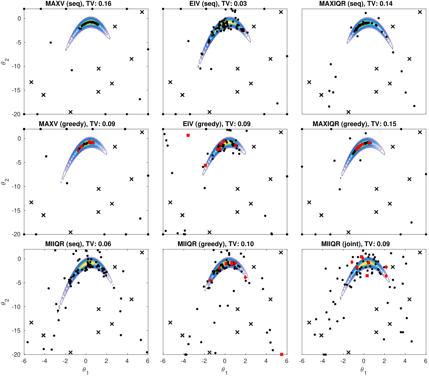 Figure 1
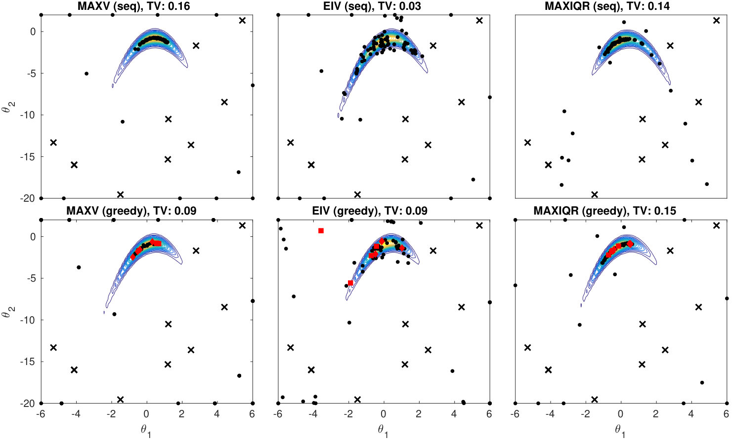 Figure 2
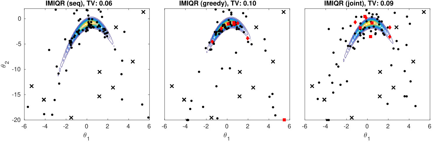 Figure 3
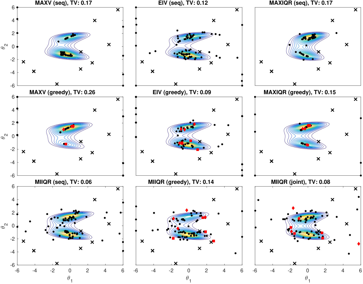 Figure 4
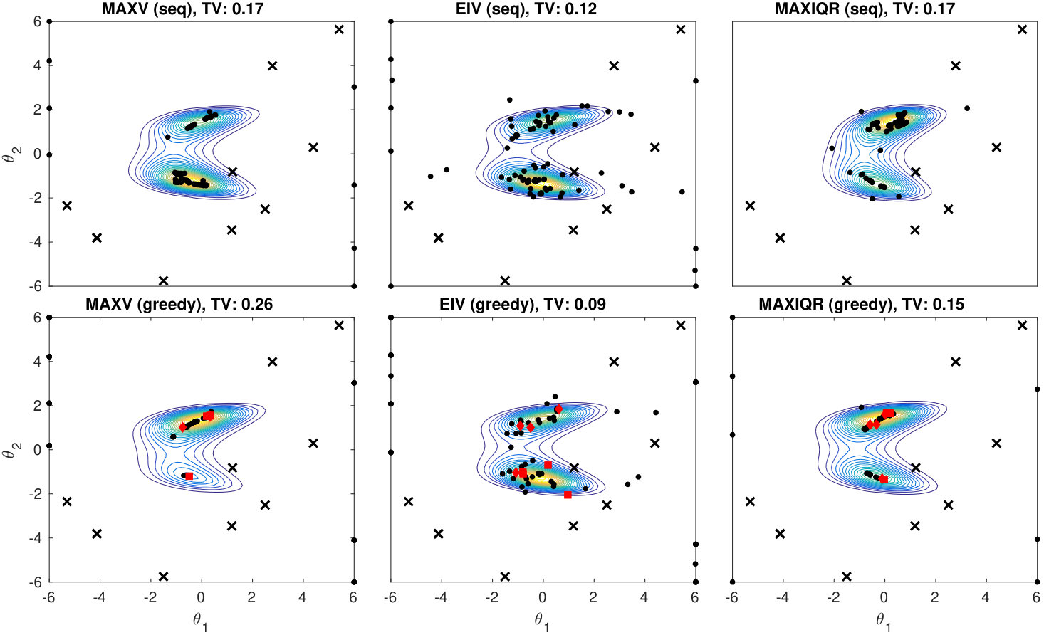 Figure 5
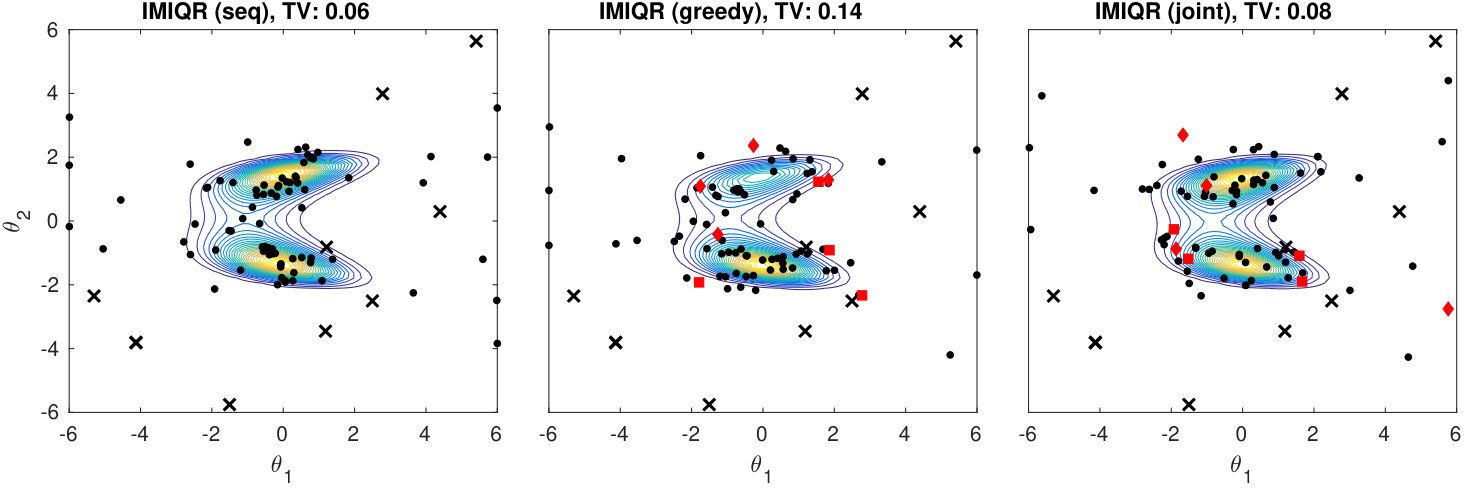 Figure 6
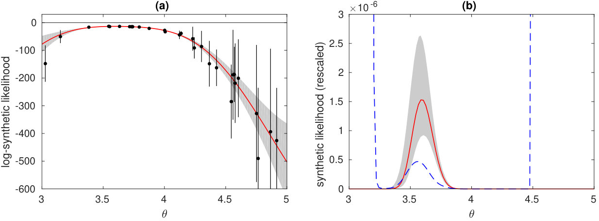 Figure 7
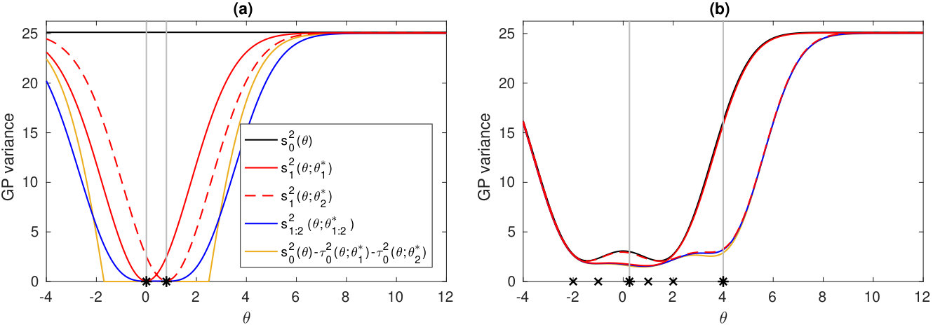 Figure 8
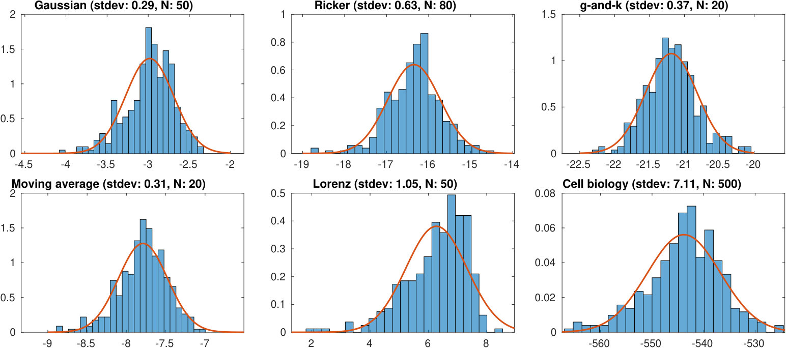 Figure 9
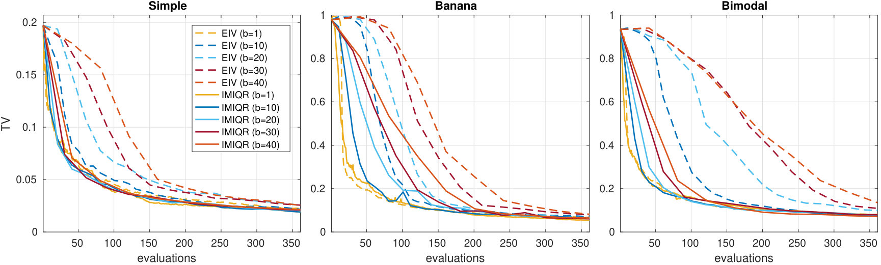 Figure 10
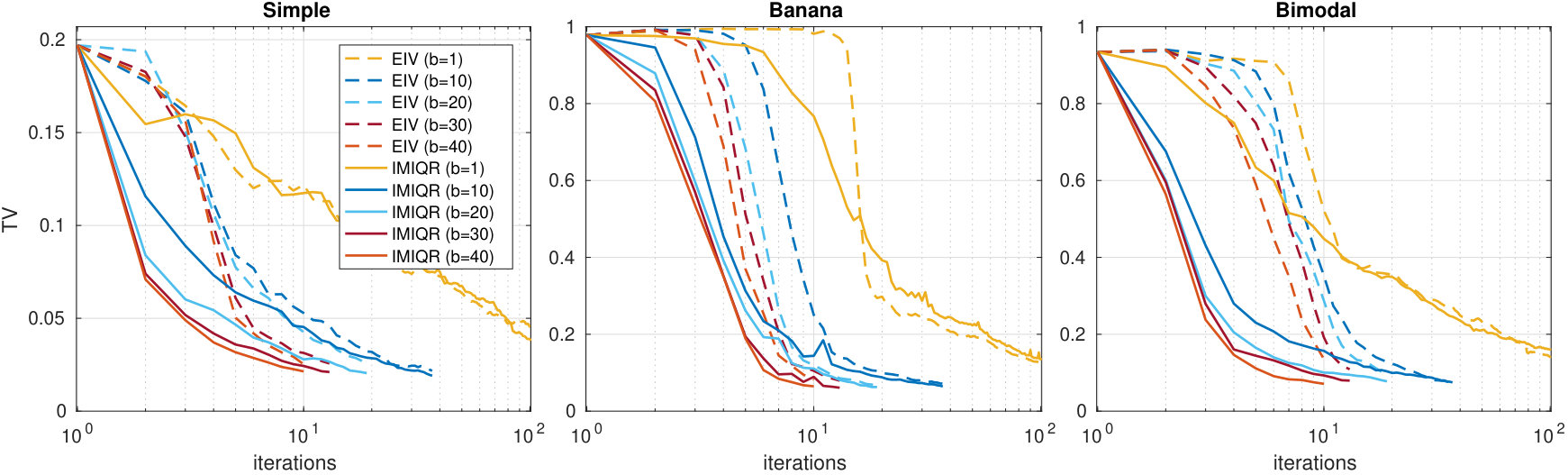 Figure 11
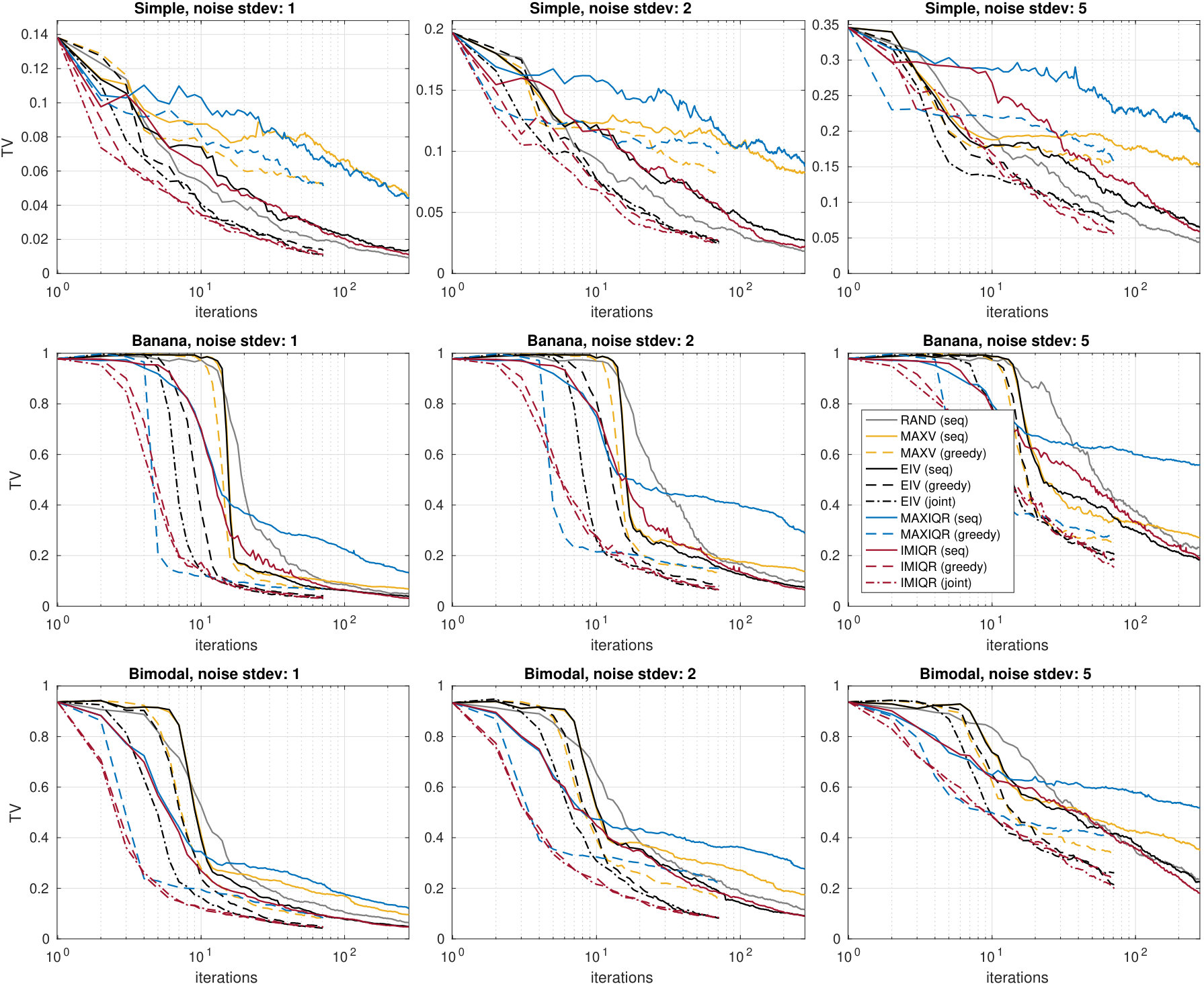 Figure 12
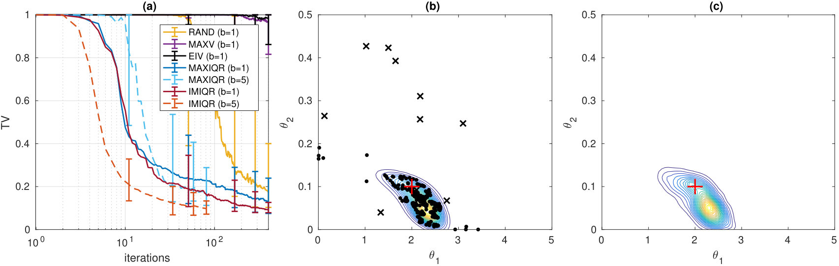 Figure 13
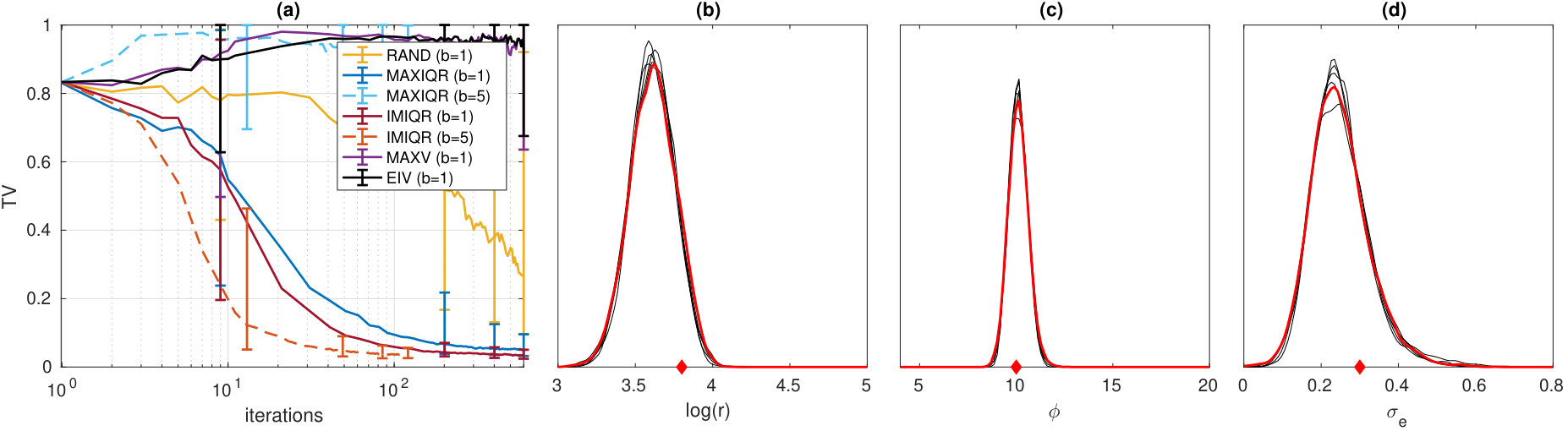 Figure 14
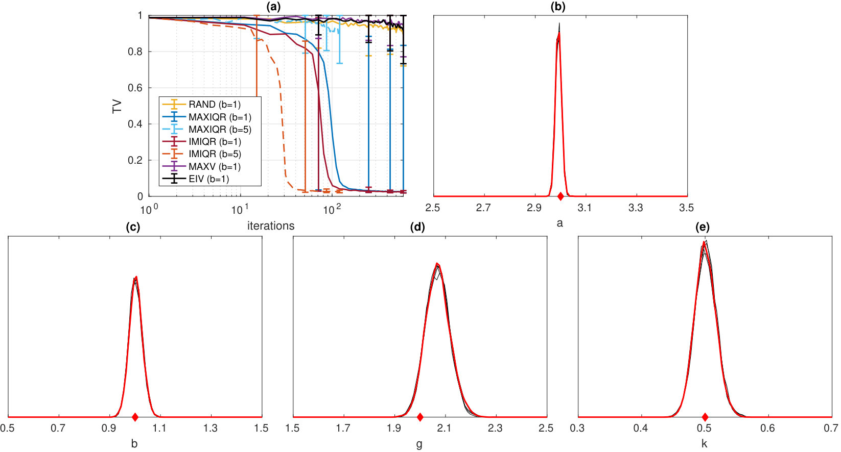 Figure 15
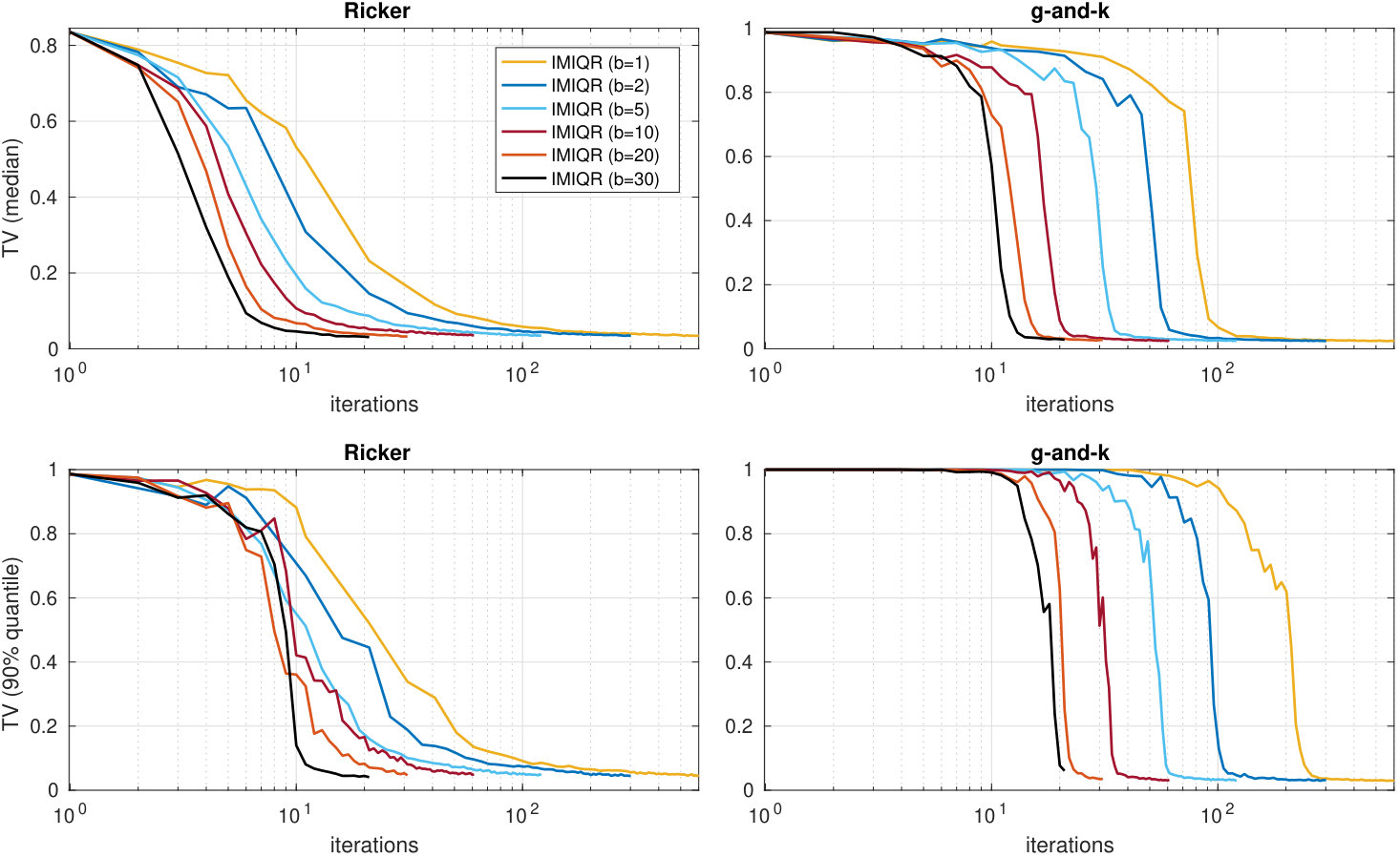 Figure 16
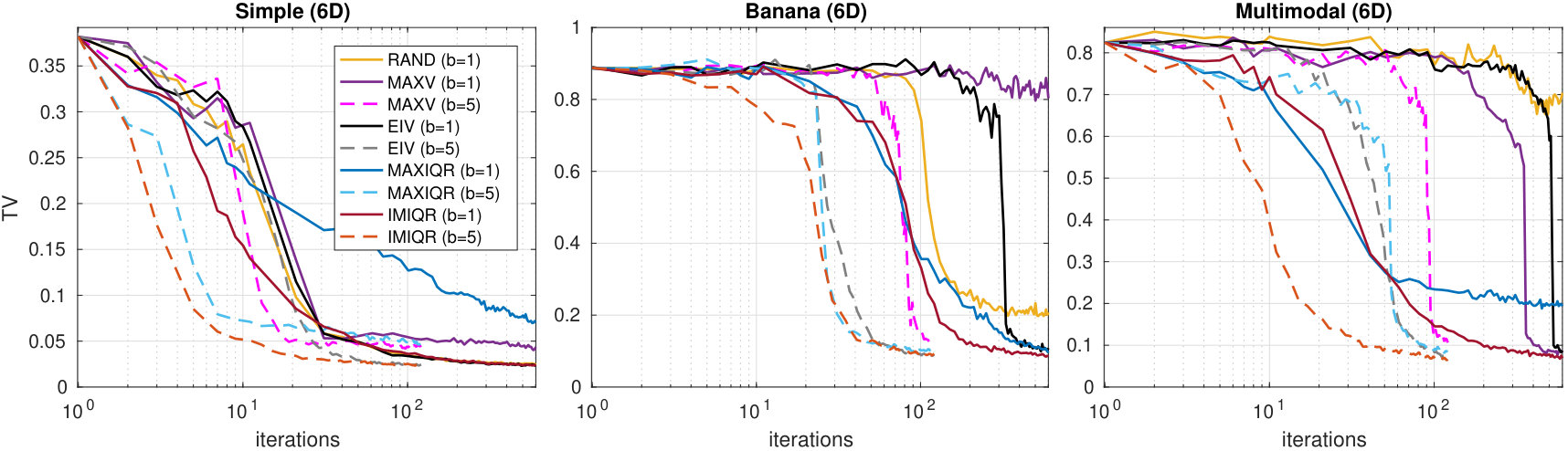 Figure 17
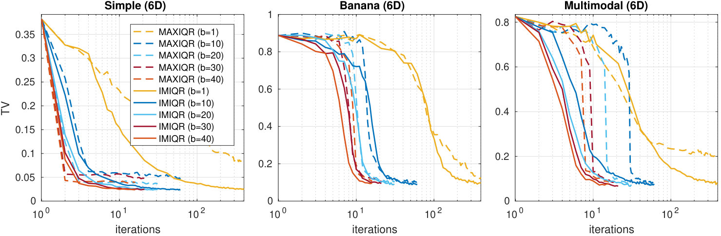 Figure 18
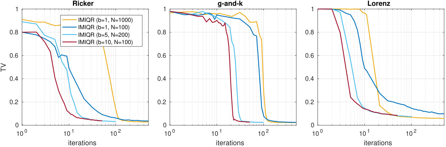 Figure 19
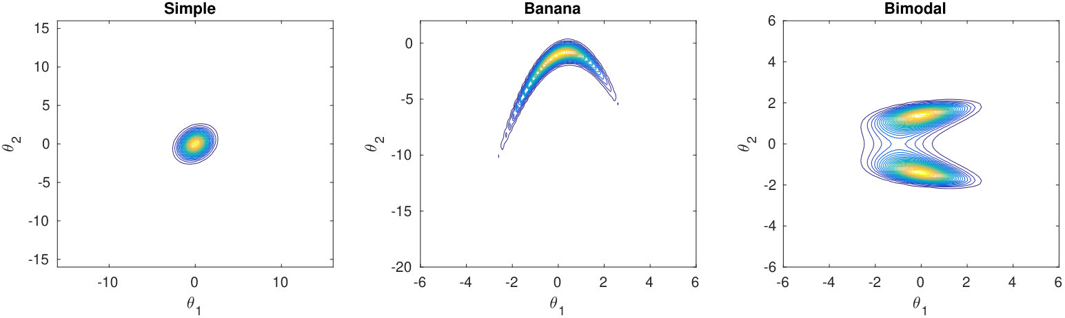 Figure 20
Peer Reviews
No public reviews on file for this paper yet. If you reviewed it on a platform where reviews are public (OpenReview, ICLR, NeurIPS, ICML), you can paste yours below so the community can read it here.
Code & Models
Videos
No videos yet. Explain this paper in a talk, walkthrough, or lecture? Add one.
Taxonomy
MethodsGaussian Process
Parallel Gaussian process surrogate Bayesian inference with noisy likelihood evaluations
Marko Järvenpää
Helsinki Institute for Information Technology HIIT, Department of Computer Science, Aalto University
Michael U. Gutmann
School of Informatics, University of Edinburgh
Aki Vehtari
Helsinki Institute for Information Technology HIIT, Department of Computer Science, Aalto University
Pekka Marttinen
Helsinki Institute for Information Technology HIIT, Department of Computer Science, Aalto University
Abstract
We consider Bayesian inference when only a limited number of noisy log-likelihood evaluations can be obtained. This occurs for example when complex simulator-based statistical models are fitted to data, and synthetic likelihood (SL) method is used to form the noisy log-likelihood estimates using computationally costly forward simulations. We frame the inference task as a sequential Bayesian experimental design problem, where the log-likelihood function is modelled with a hierarchical Gaussian process (GP) surrogate model, which is used to efficiently select additional log-likelihood evaluation locations. Motivated by recent progress in the related problem of batch Bayesian optimisation, we develop various batch-sequential design strategies which allow to run some of the potentially costly simulations in parallel. We analyse the properties of the resulting method theoretically and empirically. Experiments with several toy problems and simulation models suggest that our method is robust, highly parallelisable, and sample-efficient.
1 Introduction
When the analytic form of the likelihood function of a statistical model is available, standard sampling techniques such as Markov Chain Monte Carlo (MCMC, see e.g. Robert and Casella (2004)) can often be used for Bayesian inference. However, many models of interest in several areas of science, for example in computational biology and ecology, have an expensive-to-evaluate or intractable likelihood function which severely complicates inference. When the likelihood is intractable but forward simulation of the model is feasible, simulation-based inference methods (also called likelihood-free inference) such as approximate Bayesian computation (ABC) can be used. Unfortunately, such algorithms typically require a huge number of simulations making inference computationally costly. Examples of models with intractable likelihoods can be found in e.g. Beaumont et al. (2002); Marin et al. (2012); Lintusaari et al. (2017); Marttinen et al. (2015); Järvenpää et al. (2018) and Section 6.2 of this article.
Surrogate models, also called meta-models or emulators, such as Gaussian processes (Rasmussen and Williams, 2006) have been used extensively to calibrate deterministic computer codes, see e.g. Kennedy and O’Hagan (2001). GP surrogates have recently also been used to accelerate Bayesian inference by modelling some part of the inferential process, such as the log-likelihood function. The model allows extracting information from the simulations efficiently, and can be used e.g. to determine where additional simulations are needed. For example, Rasmussen (2003); Kandasamy et al. (2015); Sinsbeck and Nowak (2017); Drovandi et al. (2018); Wang and Li (2018); Acerbi (2018) have developed GP-based techniques to accelerate Bayesian inference when the exact likelihood or the corresponding deterministic model is tractable but expensive. Various GP surrogate techniques have been proposed also for ABC, where one can only draw samples i.e. pseudo-data from a statistical model but not evaluate the likelihood. These include Meeds and Welling (2014); Jabot et al. (2014); Wilkinson (2014); Gutmann and Corander (2016); Järvenpää et al. (2019).
In this paper we focus on GP surrogate modelling of noisy log-likelihood evaluations. Earlier works on emulating the log-likelihood function have mostly assumed exact, i.e., noiseless evaluations or the noise has not been explicitly modelled. We show that noisy evaluations cause extra challenges. Also, although not the focus of this work, we remark that one often has some control over the noise level. While our approach is applicable whenever noisy, expensive log-likelihood evaluations of a statistical model of interest are available, we mainly focus on likelihood-free inference using the synthetic likelihood method (Wood, 2010; Price et al., 2018), where the intractable log-likelihood is approximated using repeated forward simulations at each evaluation location.
Recently, Järvenpää et al. (2019) developed a Bayesian decision theoretic framework for ABC inference and considered sequential strategies (also called active learning) to select the next evaluation location for an expensive simulation model. Here we extend this framework in two ways: 1) we modify it to address the problem of Bayesian inference using noisy log-likelihood evaluations, which is different from ABC, and 2) we develop batch-sequential design strategies to efficiently parallelise the estimation of the surrogate likelihood. In earlier related works the simulation locations have been selected either sequentially (Kandasamy et al., 2015; Sinsbeck and Nowak, 2017; Wang and Li, 2018; Acerbi, 2018; Järvenpää et al., 2019) or using simple heuristics (Wilkinson, 2014; Gutmann and Corander, 2016). Batch strategies are useful when a computing cluster is available and, as we show, can substantially reduce the computation time compared to the corresponding sequential strategies. We also analyse some properties of the proposed methods theoretically, and conduct an extensive empirical comparison.
Our approach is closely related to Bayesian quadrature (BQ), see e.g. O’Hagan (1991); Hennig et al. (2015); Karvonen et al. (2018). In particular, BQ methods have been used by Osborne et al. (2012); Gunter et al. (2014); Chai and Garnett (2019) to compute the marginal likelihood and to quantify the numerical error of this integral probabilistically. In this article we are not interested in this particular integral but in obtaining an accurate estimate of the posterior. Also, we allow noisy log-likelihood evaluations. Another related problem is Bayesian optimisation (BO), see e.g. Brochu et al. (2010); Shahriari et al. (2015). Our objective to parallelise simulations is motivated by recent research on batch Bayesian optimisation (Ginsbourger et al., 2010; Azimi et al., 2010; Snoek et al., 2012; Contal et al., 2013; Desautels et al., 2014; Shah and Ghahramani, 2015; Wu and Frazier, 2016; Gonzalez et al., 2016; Wilson et al., 2018). However, while BO methods can be used to accelerate likelihood-free Bayesian inference (Gutmann and Corander, 2016), they are not specifically designed for estimating the posterior (see discussion in e.g. Kandasamy et al. (2015); Järvenpää et al. (2019)). Similarly to Järvenpää et al. (2019), we explicitly design our algorithms from the first principles of Bayesian decision theory to acknowledge the goal of the analysis, i.e. estimation of the posterior density. Finally, we note that GPs in conjuction with Bayesian experimental designs have also been successful in estimating level and excursion sets of expensive-to-evaluate functions, see e.g. Bect et al. (2012); Chevalier et al. (2014); Lyu et al. (2018).
This paper is organised as follows. Section 2 briefly reviews ABC and the SL. Sections 3 and 4 contain the details of our GP surrogate model and posterior estimation. Batch-sequential design strategies for sample-efficient estimation of the (approximate) posterior distribution are developed in Section 5 while Section 6 contains experiments. Finally, Section 7 contains discussion and concluding remarks. Proofs, implementation details and additional experiments can be found in the Appendix.
2 ABC and the synthetic likelihood methods
Our goal is to estimate parameters of a simulation model given observed data . We assume is a compact subset of and that the prior information about feasible values of is coded into a (continuous) prior pdf . For simplicity we consider only continuous parameters but discrete parameters can be handled similarly. If evaluating the likelihood function is feasible, the posterior distribution can be computed using Bayes’ theorem up to a normalisation constant and hence be used as a target distribution in MCMC. However, when the likelihood is too costly to evaluate or unavailable, standard MCMC algorithms become infeasible.
Even when the likelihood is intractable, simulating “pseudo-data” from the model, i.e., drawing samples , is often feasible. In this case, ABC can be used for inference, see e.g. Marin et al. (2012); Turner and Van Zandt (2012); Lintusaari et al. (2017). Standard ABC techniques approximate the posterior as
[TABLE]
where denotes the indicator function, is a tolerance parameter and is the discrepancy function used to compute the similarity between the simulated data and the observed data . The discrepancy is typically constructed from low-dimensional summary statistics , so that , where is, for example, the weighted Euclidean distance. For each proposed parameter , an unbiased ABC posterior estimate can be obtained by replacing the integral in (1) with a Monte Carlo sum using some simulated pseudo-data sets for .
An alternative to ABC is the synthetic likelihood method (Wood, 2010; Price et al., 2018). In SL the summary statistics are assumed to have a Gaussian distribution for each parameter , that is
[TABLE]
The first approximation results from replacing the full data with a potentially nonsufficient summary statistics . The second approximation is due to the possible violations of the Gaussianity of . The expectation and covariance matrix in (2) are unknown and are estimated for each proposed parameter using maximum likelihood (ML):
[TABLE]
where for . As investigated by Price et al. (2018), the standard Metropolis algorithm can be combined with SL. The likelihood is then computed using (2) and the ML estimates in (3) or, alternatively, using an unbiased estimate of shown in Section 2.1 of Price et al. (2018) which produces an exact pseudo-marginal MCMC if the Gaussianity assumption holds. See Appendix C for discussion on the use of different SL estimators.
The advantage of SL over ABC is that specifying suitable ABC tuning parameters such as the tolerance and the discrepancy is avoided. While the Gaussianity of the summary statistics may not hold in practice, Price et al. (2018) have found that SL is often robust to deviations from normality. SL and its extensions (Thomas et al., 2018; An et al., 2019b, a; Frazier et al., 2019) produce pointwise noisy log-likelihood evaluations because in practice the number of repeated simulations at each point is finite. Using (pseudo-marginal) MCMC or other sampling-based techniques for inference with these noisy targets thus requires a large number of simulations. Assuming noisy log-likelihood evaluations are available, e.g. obtained by using SL, the goal of the following sections is to develop an inference algorithm that can minimise the number of evaluations needed.
3 Gaussian process surrogate for the noisy log-likelihood
We denote the log-likelihood or its approximation, such as the log-SL obtained as the logarithm of (2), as . We assume that we have access to noisy log-likelihood evaluations at denoted by for building the surrogate model and that the “noise” i.e. the numerical or sampling error in evaluating the log-likelihood is independently Gaussian distributed. Treating the noisy log-likelihood evaluations as “observations”, our measurement model is
[TABLE]
where is a (continuous) function of that determines the standard deviation of the observation noise and is assumed known. To justify our model in (4), we show empirically that log-SL is well approximated by a Gaussian distribution using six benchmark simulation models in the Appendix D.1.
We place the following hierarchical GP prior for the log-likelihood function :
[TABLE]
where is a covariance function and are fixed basis functions (both assumed continuous). The nuisance parameters in (5) are marginalised, see e.g. O’Hagan and Kingman (1978); Rasmussen and Williams (2006), to obtain the following equivalent GP prior
[TABLE]
where is a column vector consisting of the basis functions evaluated at . We use basis functions of the form . A similar GP prior has been considered in Wilkinson (2014); Gutmann and Corander (2016); Drovandi et al. (2018), however, different from those articles, we take a fully Bayesian approach and marginalise as in Riihimäki and Vehtari (2014). Since little initial information is typically available on the magnitude and shape of the log-likelihood, we use relatively uninformative hyperpriors so that and . We assume that the log-likelihood function is smooth, and adopt the squared exponential covariance function although other choices, such as the Matérn covariance function, are also possible. We denote the covariance function hyperparameters as . For now, we assume is known and omit it from our notation for simplicity.
Given observations , which we call training data, our knowledge of the log-likelihood function is , where
[TABLE]
with for , ,
[TABLE]
and . Above is the matrix whose columns consist of basis function values evaluated at training points which is itself a matrix, and is the corresponding vector at test point . From now on, we denote the GP variance function as and the probability law of given as , that is, .
4 Estimators of the posterior from the GP surrogate
Using the GP surrogate model for the noisy log-likelihood, we here derive estimators for the posterior which can be e.g. plugged-in to a MCMC algorithm. Resulting sampling algorithms do not require further simulator runs (unlike e.g. SL-MCMC) producing potentially huge computational savings. Figure 1 demonstrates our approach. We want to use our knowledge of the log-likelihood function represented by to determine the optimal point estimate of the probability density function (pdf) of the posterior111While in this article we are mainly concerned with point estimators of the posterior pdf, we can also quantify its (epistemic) uncertainty similarly to probabilistic numerics literature (see e.g. Hennig et al. (2015); Cockayne et al. (2019); Briol et al. (2019)) as illustrated in Figure 1b. Such uncertainty estimates are also used to intelligently select the next simulation locations in Section 5.. The uncertainty of the log-likelihood can be propagated to the posterior distribution of the simulation model which consequently becomes a random quantity denoted as :
[TABLE]
The expectation of the posterior pdf at each parameter can be formally written as
[TABLE]
and the variance can be obtained similarly (assuming these quantities exist). In principle, one could sample posterior pdfs by first drawing (a continuous function ), then computing , and finally normalising. However, in practice this would require discretisation of the -space and involves computational challenges. For this reason and similarly to Sinsbeck and Nowak (2017); Järvenpää et al. (2019), we instead take our quantity of interest to be the unnormalised posterior
[TABLE]
which follows log-Gaussian process that allows analytical computations.
Next we derive an optimal estimator for the unnormalised posterior in (12) using Bayesian decision-theory. We proceed here similarly to Sinsbeck and Nowak (2017) and consider the integrated quadratic loss function between two (unnormalised) posterior densities and . We assume and are square-integrable functions in , i.e. . The optimal Bayes estimator, denoted by , is the minimiser of the expected loss, where denotes the set of candidate estimators. In detail,
[TABLE]
where Tonelli theorem is used to change the order of expectation and integration and where is a candidate estimator of . Equation 13 shows that the expected loss is minimised when the integrand on the second row is minimised independently for (almost) each . It follows from the basic results of Bayesian decision theory (see e.g. Robert (2007)) that the minimum is obtained when , i.e., the optimal estimator is the posterior expectation. The minimum value of (13), called Bayes risk, is the integrated variance . The posterior expectation and variance can be computed from the log-Normal distribution as
[TABLE]
If we instead use loss where , we can similarly show that the optimal point estimator is the marginal median. The median and the quantile with can be computed as
[TABLE]
where is the quantile function of the standard normal distribution. As we show in the Appendix A, the Bayes risk corresponding to the loss is
[TABLE]
When MCMC is used with the point estimator of the unnormalised posterior in either (14) or (15), we are in fact targeting the following mean and median based estimators of the (normalised) posterior
[TABLE]
These are obtained by simply normalising the Bayes optimal estimators of the unnormalised posterior (and, as a consequence, a guarantee of optimality for normalised posterior does not follow). Similar estimators were also considered by Stuart and Teckentrup (2018). Both are clearly valid density functions, and tractable, unlike (11). The latter, i.e., the marginal median based estimate, is equal to (10) if we replace the unknown log-likelihood function with a GP mean function and neglect GP uncertainty. On the other hand, the former, i.e., the marginal mean estimate, takes into account the GP uncertainty through the variance function . These two point estimates become the same if the GP variance is negligible.
5 Parallel designs of simulations
In the previous section we showed how to quantify the uncertainty of the GP surrogate-based unnormalised posterior density and we derived computable and (in a certain sense) optimal point estimates of it. Next we develop Bayesian experimental design strategies to select further locations to evaluate the log-likelihood, so that the uncertainty in the unnormalised posterior decreases as fast as possible. We focus on batch strategies and denote the batch size as . Before moving on, we introduce some terminology. The next batch of evaluation locations is obtained as the solution to an optimisation problem. We call the objective function of this optimisation problem a design criterion and the resulting batch of evaluation locations as design points or just design. The complete procedure of selecting the design points is called a batch-sequential (or, when , just sequential) strategy222The design criterion is often called an acquisition function and the resulting strategy sometimes an acquisition rule in the BO literature..
In this paper we focus on syncronous parallelisation where a batch of design points is constructed at each iteration and the corresponding simulations are simultaneously submitted to the workers. However, the “greedy” design strategies developed in Sections 5.3 and 5.5 can also be used for asyncronous parallelisation, where a new location is immediately chosen and submitted for processing, whenever any of the running simulations completes, instead of waiting all the other simulations to finish.
5.1 Analytical expressions for the design criteria
We first derive some general results needed for efficient evaluation of the design criteria. These can be useful also for developing batch designs for other related GP-based problems such as BQ and BO. Given it is useful to know how additional candidate evaluations at points would affect our knowledge about the log-likelihood and the unnormalised posterior . The following Lemma is central to our analysis. It shows how the GP mean and variance functions are affected by supplementing the training data with a new batch of evaluations when the unknown is assumed to be distributed according to the posterior predictive distribution of the GP given . The Lemma is a generalisation of a similar result by Järvenpää et al. (2019); Lyu et al. (2018).
Lemma 5.1**.**
Consider the mean and variance functions of the GP model in Section 3 for a fixed , given the training data and when treated as functions of . Assume follows the posterior predictive distribution, that is . Then,
[TABLE]
where is the Dirac measure and
[TABLE]
In the Lemma, is the GP mean function at iteration whose dependence on is shown explicitly. Importantly, the above Lemma shows how the GP variance decreases from to when the extra evaluations at are included, and the reduction is deterministic. We see, for example, that if for all which might hold approximately, e.g., if the evaluation points are located far from each other, then
[TABLE]
This shows that the reduction of GP variance at , , factorises over the new evaluation points in . Intuitively, if the test point is strongly correlated with some evaluation point , including the evaluation at will result in a large reduction of variance at the test point. Furthermore, the larger the noise variance at the evaluation point is, the less the GP variance will decrease.
It clearly holds that . Items (i-ii) of the following Lemma summarise some additional properties of the variance reduction function in (20) and (iii-iv) show two further useful identities needed later. Item (i) shows the (rather obvious) result that the order of evaluation points in does not change and in the following we often identify the matrix with a multiset whose elements are the columns of although this leads to some abuse of notation.
Lemma 5.2**.**
Let and let be any test point. The function in (20) for any fixed has the following properties.
- (i)
The function value is invariant to the permutation of the evaluation locations i.e. the columns of . 2. (ii)
Let . Then , i.e., including new evaluations never increases variance. 3. (iii)
Let so that and denote the predictive variance at by for . Then
[TABLE] 4. (iv)
Let where and , and denote . Then
[TABLE]
Figure 2 demonstrates how two new evaluations at and reduce the GP variance in two different one-dimensional examples. Specifically, Figure 2a illustrates the fact of Lemma 5.2 (iii) that the interaction between the evaluation points, represented by the term , affects the reduction of the GP variance and its effect can be either positive or negative (the variance after two new evaluations, blue line, is either below or above the yellow line, which represents the reduced variance if the interaction is neglected). In Figure 2b the new evaluation locations are far apart and the factorisation of the variance reduction in (21) holds approximately.
5.2 Batch-sequential designs
Given , our goal is to select the next batch of evaluations in an optimal fashion. We take a Bayesian decision theoretic approach, where is selected to minimise the expected (or median) loss, where the loss measures uncertainty remaining in the unnormalised posterior when the hypothetical observations at locations are taken into account. In the following we develop two such techniques based on two different measures of uncertainty: variance and interquartile range (IQR). Design strategies which acknowledge the impact of the next batch, but neglect the whole remaining computational budget, are often called “myopic”. It is possible to formulate a non-myopic design as a dynamic programming problem, but this is computationally demanding, see e.g. Bect et al. (2012); González et al. (2016). Consequently, we focus on myopic designs which already produce highly sample-efficient and practical algorithms.
5.2.1 Expected integrated variance (EIV)
As our first measure of the uncertainty of the unnormalised posterior for the selection of the next batch design , we select the Bayes risk under the loss. In this case, the Bayes risk is the integrated variance function
[TABLE]
whose integrand was obtained from (14). This is similar to Sinsbeck and Nowak (2017); Järvenpää et al. (2019) who, however, considered other GP surrogate models and only sequential designs. We compute the expectation over the hypothetical noisy log-likelihoods for any candidate design , leading to the expected integrated variance design criterion (EIV). The resulting optimal strategy is a special case of stepwise uncertainty reduction technique, see e.g. Bect et al. (2012). This criterion is evaluated efficiently without numerical simulations from the GP model, using the following result.
Proposition 5.3**.**
With the assumptions of Lemma 5.1, the expected integrated variance design criterion at any candidate design is
[TABLE]
5.2.2 Integrated median interquartile range (IMIQR)
A sequential design strategy based on EIV worked well in the ABC scenario of Järvenpää et al. (2019), who modelled the discrepancy in (1) with a GP. In this article we instead model the log-likelihood with a GP as illustrated in Figure 1 and the goal is to minimise the uncertainty of the unnormalised posterior , which has a log-Normal distribution for a fixed . However, the expectation and variance can be suboptimal estimates of the central tendency and uncertainty of a heavy-tailed distribution such as log-Normal. For example, Figure 1b shows that the standard deviation (dashed blue line) grows very rapidly at the boundaries although at the same time the credible interval clearly indicates that the probability of the log-likelihood, and consequently the likelihood, of having a non-negligible value there is vanishingly small. The mean is similarly affected in a non-intuitive way by the heavy tails: It is fairly easy to see that
[TABLE]
This means that with a sufficiently large variance of the log-likelihood , the probability that the likelihood is greater than its own mean becomes negligible.
The above analysis suggests (and empirical results in Section 6 further confirm) that mean-based point estimates and variance-based design strategies, such as the EIV and those proposed by Gunter et al. (2014); Kandasamy et al. (2015); Sinsbeck and Nowak (2017); Järvenpää et al. (2019); Acerbi (2018), are unsuitable when log-likelihood evaluations are noisy. A reasonable alternative for the -loss used to derive the EIV is to measure the uncertainty in the posterior using the -loss, which is less affected by extreme values. As shown in Section 3, the -loss leads to the marginal median estimate for the posterior, . While the -loss produces a robust median estimator that we adopt, (16) shows that the Bayes risk with loss scales as since for large , such that also this measure for overall uncertainty of is affected by the heavy tails of the log-Normal distribution.
We propose a new, robust design criterion for selecting the next design. In place of the variance in EIV, we use a robust measure of uncertainty, the interquartile range . The integrated IQR loss measuring the uncertainty of the posterior pdf is defined as
[TABLE]
where and for is the hyperbolic sine, which emerges after using (15). While we use , other quantiles are also possible. A theoretical downside of the IQR loss is that it does not formally coincide with the Bayes risk for the or loss, which correspond to the optimal point estimators of the unnormalised posterior (see Section 4).
We also use the median in place of the mean to measure the effect of the next design to the loss function. That is, we use median loss decision theory (see Yu and Clarke (2011)), and define the median integrated IQR loss function as
[TABLE]
The median integrated IQR loss in (29) is intractable but it can be approximated by the integrated median IQR loss (IMIQR). This approximation333Instead of approximation, which may be inaccurate when the GP variance function is large, the integrated median criterion in (30) can be seen as an alternative decision-theoretic formulation with infinitely many dependent variables of interest (one for each ) and where the median outcomes after considering the effect of the design are all computed separately for each , and the corresponding losses are combined through averaging. The median integrated loss in (29) instead has a single combined loss function. follows by replacing the predictive distribution of with a point mass, i.e., . This approximation resembles the so-called kriging believer heuristic in Ginsbourger et al. (2010). The next result gives a useful formula to calculate IMIQR.
Proposition 5.4**.**
With the assumptions of Lemma 5.1, the integrated median IQR loss, denoted as , at any candidate design is
[TABLE]
The integrand of (30) is recognised as a product of the marginal median estimate of the posterior in (15) and the function . Hence, to minimise IMIQR, the simulation locations need to be chosen as a compromise between regions where the current posterior estimate is non-negligible and where the GP variance decreases efficiently when the simulations are run at . Similar interpretation holds also for the EIV function in (26). However, EIV assigns significantly more weight to areas with high GP variance than IMIQR.
5.3 Joint and greedy optimisation for batch-sequential designs
We can now evaluate EIV and IMIQR design criteria for any candidate design and choose as the minimiser, i.e.,
[TABLE]
where is either the EIV in (26) or IMIQR in (30). The objective function is typically smooth but multimodal so global optimisation is needed. We call (31) as “joint” optimisation which does not scale to high dimensional parameter spaces or to large batch sizes. Even if computing the design criterion is cheap as compared to the run times of typical simulation models, solving the -dimensional global optimisation problem is often impractical as discussed in Wilson et al. (2018). Hence, we consider greedy optimisation as also used in batch BO (Ginsbourger et al., 2010; Snoek et al., 2012; Wilson et al., 2018). The greedy optimisation procedure for both EIV and IMIQR works as follows: the first point is chosen as in the sequential case i.e. by solving (31) with . The rest of the points are obtained by iteratively solving
[TABLE]
This greedy approach simplifies the difficult -dimensional optimisation into separate -dimensional problems, and makes it scalable as a function of .
In general, the design found by the greedy optimisation does not equal the minimiser of the joint criterion. It follows from Lemma 5.2 (i) that both EIV and IMIQR are invariant to the order of evaluation locations in but this does not hold for the greedy procedure. Bounds for the performance of greedy maximisation of a set function have been studied in literature, see e.g. Nemhauser et al. (1978); Krause et al. (2008); Bach (2013). For example, if the design criterion (when defined equivalently using a utility so that (32) becomes a maximisation problem) is submodular and non-decreasing in batch size , then the worst-case outcome of greedy optimisation is at least of the corresponding optimal joint value. A utility function corresponding to IMIQR defined below is not submodular but an approximation of it is weakly submodular (see e.g. Krause et al. (2008); Krause and Cevher (2010)). We use this fact to derive a weaker but still useful bound.
We here consider an approximation of so that
[TABLE]
which follows from the observation that and where we had . The approximation in (33) is reasonable when in the region where is non-negligible. For simplicity, we consider a discretised setting where the optimisation is done over a finite set and define (approximate) IMIQR utility function as
[TABLE]
for . Clearly, maximising is equivalent to minimising . The following theorem gives a bound for the greedy optimisation of the (approximate) IMIQR utility function. The proof can be found in Appendix B.2.
Theorem 5.5**.**
Consider the set function in (34). Let be a (joint) optimal solution for maximising over . The greedy algorithm for this maximisation problem outputs a set satisfying
[TABLE]
Computing explicitly is difficult but we expect that often since given by (23) tends to be small. However, may not always be small, the term scales quadratically for batch size , and the bound holds only approximately for IMIQR. This bound still suggests that, at least in some iterations of the algorithm, greedy IMIQR produces near-optimal batch locations. On the other hand, an approximation similar to (33) for EIV would be reasonable in a very limited number of situations, and experiments in Appendix D.3 suggest that greedy EIV scales worse as a function of compared to the corresponding greedy IMIQR strategy. Finally, we note that even when the bound is weak, new design points cannot increase the value of EIV or IMIQR loss function as shown in Appendix B.1. Hence, the batch strategies cannot be worse than the corresponding sequential designs and, in practice, they are highly useful as is seen empirically in Section 6.
5.4 Implementation details
Using the GP surrogate model and the analysis from the previous sections, we show the resulting inference method as Algorithm 1. Some key implementation details are discussed below and further details (e.g. on handling GP hyperparameters, MCMC methods used, and optimisation of the design criteria) are given in Appendix C. The algorithm is shown for the SL case using the IMIQR strategy, but it works similarly for EIV, heuristic designs developed in the next section and other log-likelihood estimators besides SL. The potentially expensive simulations on the lines 2-5 and 18-21 can be done in parallel. In the SL case, the simulations can be parallelised in terms of both the number of repeated simulations and batch size .
Evaluation of EIV and IMIQR requires numerical integration over . Similar computational challenges emerge also in the state-of-the-art BO methods such as Hennig and Schuler (2012); Hernández-Lobato et al. (2014); Wu and Frazier (2016) and in Chevalier et al. (2014). If we discretise the parameter space and approximate the integral in the resulting grid. In higher dimensions, we use self-normalised importance sampling (IS) as in Chevalier et al. (2014); Järvenpää et al. (2019). Specifically, we draw samples from the importance distribution and use these as integration points to approximate
[TABLE]
where the integrand of either (26) or 30 is denoted by . As the proposal we use the current loss (see (14) and the integrand of (16)), which is a function , and can be interpreted as an unnormalised pdf. This is a natural choice because the current loss has a similar shape as the expected/median loss as a function of . We use the same proposal in the greedy optimisation in (32) although it would be also possible to adapt the proposal according to the pending points when optimising with respect to the th point .
We have assumed that the noise function in (4) is known. In practice, this is a valid assumption only in the noiseless case where . As our focus is on the noisy setting, we need to estimate . Sometimes can be assumed to be an unknown constant to be determined together with the GP hyperparameters using MAP estimation. However, we observed that often depends on the magnitude of the log-likelihood (see Figure 1), making the assumption of homoscedastic noise questionable. Similarly to Wilkinson (2014), we estimate using the bootstrap. Specifically, with each new training data point , we resample with replacement summary vectors from the original population for times. We then compute the empirical variance of the resulting log-SL values and use it as a plug-in estimator for .
For EIV, IMIQR and greedy batch versions of MAXV and MAXIQR (see Section 5.5), needs to be also known at candidate design points . Bootstrap cannot be used because the simulated summaries are only available for training data. We take a pragmatic approach and set at the candidate design points as if the future evaluations were almost exact. This simplification effectively reduces the occurrence of (potentially redundant) simulations at nearby points to encourage exploration. Alternatively, one could use another GP to model the bootstrapped variances or their logarithms and use the GP mean function as a point estimate for the function as in Ankenman et al. (2010).
5.5 Alternative heuristic designs strategies
Here we present some heuristic alternative design strategies. These are empirically compared to the more principled EIV and IMIQR strategies in Section 6. We first focus on sequential designs where .
MAXIQR: A natural and simple approach is to evaluate where the current variance, IQR or some other suitable (local) measure of uncertainty is maximised. Such strategies are in some contexts called “uncertainty sampling”. The advantage over EIV and IMIQR is cheaper computation because the effect of the candidate design point to the whole posterior is not acknowledged. Using IQR produces the design strategy
[TABLE]
which we abbreviate as MAXIQR because it evaluates at the maximiser of IQR. Taking the logarithm of (38), the MAXIQR strategy can be equivalently written as
[TABLE]
which shows a tradeoff between evaluating where the log-posterior is presumed to be large (the first two terms in (39)) and unexplored regions where the GP variance is large (the last two terms). This formula also shows an interesting connection to the upper confidence bound (UCB) criterion commonly used in BO, see e.g. Srinivas et al. (2010); Shahriari et al. (2015). The UCB acquisition function is , where is a tradeoff parameter, here automatically chosen to be . Compared to the standard UCB, there is, however, an extra term in (39) which further penalises regions having small variance . If the variance is large everywhere and/or if is an extreme quantile, then the last term in (39) is approximately zero and the MAXIQR design criterion approximately equals UCB.
MAXV: When the variance is used instead of IQR, we obtain a strategy
[TABLE]
This strategy is abbreviated as MAXV which, in fact, is used by Gunter et al. (2014); Kandasamy et al. (2015) in the noiseless case, and it is called “exponentiated variance” by Kandasamy et al. (2015). Taking logarithm of (40) shows that this design also features a tradeoff between large posterior and large variance, similarly to MAXIQR.
Since these two strategies are not derived from Bayesian decision theory, it is not immediately clear how one should parallelise these inherently sequential strategies. However, it seems reasonable to use the fact the is always reduced near the pending evaluation locations. Motivated by this and related BO techniques in Ginsbourger et al. (2010); Snoek et al. (2012); Desautels et al. (2014), we compute the median value of the design criterion with respect to the posterior predictive distribution of the pending simulations. The next locations are chosen iteratively such that, for MAXIQR, the first point in the batch is chosen using (38) and the rest by iteratively solving
[TABLE]
MAXV is parallelised similarly but using the expected value instead of the median.
Finally, we provide some intuition to (41) and show a connection to the local penalisation method used to parallelise sequential BO designs by Gonzalez et al. (2016). Suppose we are selecting the th point of a batch where . Comparison of (38) and (41) shows that (41) equals the original design criterion in (38) multiplied by a weight function . It is easy to see that . This shows that when we take the median over the log-likelihood evaluation at the pending points , we are implicitly making the original acquisition function smaller around the pending points and, consequently, penalising additional evaluations there. This resembles the heuristic method by Gonzalez et al. (2016), who proposed to multiply the non-negative acquisition function, such as the objective of (38), with , where are local penalising functions around the pending evaluation locations , when selecting the th point of the current batch. However, one difference between these approaches is that our weight function takes the interactions between the pending points into account and it cannot be factorised as . Also, our weight function is not a tuning parameter but follows automatically from our analysis.
6 Experiments
We empirically investigate the performance of the proposed algorithm with different design strategies developed in Section 5. We compare the sequential, batch, and greedy batch strategies based on EIV and IMIQR to sequential and greedy versions of MAXV (which is essentially the same as the BAPE method by Kandasamy et al. (2015)) and MAXIQR. As a simple baseline we also sample design points from the prior (always uniform) and this method is abbreviated as RAND.
We report the results as figures whose y-axis shows the accuracy between the estimated and the ground truth posterior using total variation distance (TV). TV between pdfs and is defined as and is computed using numerical integration in 2D. In higher dimensional cases we compute the average TV between the marginal posterior densities using MCMC samples. The marginal median estimator in (17) is used to obtain the point estimate for the posterior pdf. The x-axis represents the iteration of the Algorithm 1 (unless explicitly stated otherwise) which serves as a proxy to the total wall-time when the noisy likelihood evaluations are assumed to dominate the total computational cost. We use a fixed simulation budget so that the batch-sequential methods terminate earlier than the sequential ones because they spend the evaluation budget times faster due to the parallel computation.
We consider two sets of experiments: toy models where noisy log-likelihood evaluations are directly evaluated (Section 6.1) and real-world simulator-based statistical models where SL is used to obtain noisy log-likelihood evaluations using repeated simulations at each proposed parameter (Section 6.2). Although in the SL case it is often possible to adjust adaptively, we use (unless explicitly stated otherwise) for simplicity. In the Appendix D.4 we show that our batch methods are beneficial for SL even though in principle it would be possible to directly parallelize the simulations themselves. For example, when computer cores are available for the simulations (e.g. in a high performance computing cluster), it is beneficial to use the batch strategies (e.g. and ) instead parallelizing the evaluations at a single location ( and ). More elaborate analysis of resource allocation is left for future work. A MATLAB implementation of our algorithms is available at https://github.com/mjarvenpaa/parallel-GP-SL.
6.1 Noisy toy model likelihoods
We first define three 2D densities with different characteristics: a simple Gaussian density called ’Simple’, a banana-shaped density ’Banana’ and a bimodal density ’Bimodal’. We then construct three 6D densities so that their 2D blocks are independent and have the corresponding 2D densities as their 2D marginals. Detailed specification and illustrations can be found in Appendix D.2. We use the same names for the 6D densities as for the corresponding 2D ones (except that ’Bimodal’ is called ’Multimodal’ in 6D because it has modes). The independence assumption is not taken into account in the GP model to make the inference problem more challenging. For simplicity, is assumed constant i.e. it does not depend on the magnitude of the log-likelihood and its value is obtained using MAP estimation together with other GP hyperparameters at each iteration in Algorithm 1. As an initial design in 6D we generate parameters (’Simple’) or (’Banana’ and ’Multimodal’) from uniform priors. In the 2D case we always use . We use a fixed total budget of noisy log-likelihood evaluations (’Simple’) or (’Banana’ and ’Multimodal’) for both sequential and batch methods in 6D.
The results with different sequential and greedy batch-sequential strategies in 6D case with batch size are shown in Figure 3. Good posterior approximations for the Simple example are obtained earlier than for the two other models. This is a consequence of the quadratic terms in the GP prior mean function and the exact Gaussian shape of the posterior. However, more complicated posteriors are also estimated accurately although more iterations are needed to obtain reasonable approximations. The IMIQR method works clearly the best outperforming EIV and the heuristic MAXV and MAXIQR methods which either need more iterations to obtain good approximation or fail completely to reach good results. The uniform design RAND works adequately in the Simple and Banana models but often produces poor estimates for the Multimodal case. Unsurprisingly, its performance is also poor in the real-world scenarios in Section 6.2.
The batch-sequential strategies improve the convergence speed as compared to the corresponding sequential strategies in all cases of Figure 3. In particular, the greedy batch versions of MAXV and MAXIQR even outperform the corresponding sequential methods. The greedy batch strategy in these cases encourages exploration as compared to the corresponding sequential strategy and this effect counterbalances the exploitative nature of MAXV and MAXIQR. In Appendix D.3 we compare the joint and greedy batch strategies in 2D case where joint maximisation is still feasible. Their difference is found small for IMIQR and small or moderate for EIV suggesting that the greedy strategies are in practice nearly optimal.
Figure 4 and further examples in the Appendix D.3 illustrate the design points and estimated posteriors for various design strategies in 2D case. An important observation is that MAXV and IMIQR are exploitative i.e. they produce points near the mode of the posterior where the local measure of uncertainty they use tend to be highest. Also, in general, the sequential and batch methods produce similar designs. However, greedy MAXIQR generates more points on the boundary than the corresponding sequential strategy and the joint IMIQR produces slightly more diverse design points as the sequential and greedy batch IMIQR. In all cases, IMIQR avoids redundant evaluations on the boundaries.
We investigate the effect of batch size in the greedy batch MAXIQR and MAXIQR algorithms in Figure 5. In general, the convergence speed of both methods scales well as a function of and already yields useful improvements. However, increasing over would improve the results only slightly. Greedy batch IMIQR works overall better than batch MAXIQR. The variability in the posterior approximations produced by IMIQR is small in all cases unlike for MAXIQR which occasionally produced poor approximations (not shown for clarity). In the Appendix D.3 we compare EIV and IMIQR in 2D. These results show that the greedy IMIQR batch-sequential strategy outperforms the corresponding EIV strategy although their difference is small in the corresponding sequential cases. This suggests that, even when is small so that the variance in EIV serves as a reasonable measure of uncertainty and the sequential EIV works similarly to IMIQR, the greedy batch median-based IMIQR design strategy better mimics the sequential decisions than EIV.
6.2 Simulation models
We perform experiments with three benchmark problems used previously in the ABC literature. Two of these are shown here and the third one in the Appendix D.5. While the proposed methodology is particularly useful for expensive simulation models, we however consider only relatively cheap models as this allows to repeat the computations many times with different realisations of randomness to assess the variability and robustness, and to conduct accurate comparisons to reasonable ground truth posteriors. Nevertheless, these experiments serve as examples of challenging real-world inference scenarios where the GP and SL modelling assumptions do not hold exactly. In each problem, we set the unknown parameter of the simulation model to a value used previously in the literature and generated one data set from the simulation model using this “true” parameter. The posterior used as the ground truth was computed using SL-MCMC. Multiple chains each with length were used to ensure that the variability due to Monte Carlo error was small.
6.2.1 Ricker model
We first consider the Ricker model presented in Wood (2010). In this model denotes the number of individuals in a population at time which evolves according to the discrete time stochastic process for , where . The initial population size is . It is assumed that only a noisy measurement of the population size at each time point is available with the Poisson observation model Given data , the goal is to infer the three parameters . We use the uniform prior . The same summary statistics as in Wood (2010); Gutmann and Corander (2016); Price et al. (2018) are used to compute log-SL evaluations. The number of repeated simulations is fixed to . The “true” parameter to be estimated is and it is used to generate the observed data with length . The initial training data size is and the additional budget of simulations is so that the total budget is SL evaluations corresponding simulations. The integrals of EIV and IMIQR are approximated using IS and is estimated using bootstrap as described in Section 5.4.
Figure 6 shows the results. We see that the EIV and MAXV strategies perform poorly. These strategies tend to evaluate where the variance of the posterior is high, although as discussed in Section 5, these do not necessarily correspond to the regions with non-negligible likelihood. In fact, the magnitude of the log-likelihood and its noise variance grow fast near the boundaries of the parameter space where the chaotic nature of the model also makes the log-likelihood surface irregular which further causes difficulties with GP modelling. The IMIQR method again produces the best posterior approximations which are comparable to the true SL posterior. Some examples are shown in Figure 6b-d. Also, MAXIQR method works well on average but it produces less coherent results than IMIQR which is likely the result of its exploitative nature. In addition, unexpectedly, the greedy MAXIQR method performs poorly. The probable reason is that the batch evaluations become too diverse having many evaluations in the boundary which leads to poor GP fitting and subsequently poor future designs. However, the robust batch-sequential IMIQR method with works as expected producing useful improvement to the convergence speed as compared to sequential IMIQR.
6.2.2 g-and-k model
We consider the g-and-k distribution as in Price et al. (2018). The g-and-k model is a flexible probability distribution defined via its quantile function
[TABLE]
where and are parameters and is a quantile. We fix and estimate the parameters using a uniform prior . We use the same four summary statistics as Price et al. (2018) who fitted an auxiliary model, skew t-distribution, to the set of samples generated from (42) using maximum likelihood, and took the resulting skew t score vector at the ML estimate as the summary statistic. Although there are only summary statistics, we again use . We use the same settings as for the Ricker model except that the initial design is increased to so that the total budget is SL evaluations. The true value of the parameter is chosen to be .
Overall, the results in Figure 7 are similar to those of the Ricker model. However, the larger parameter space slows down the convergence speeds initially as expected, as compared to the Ricker model. Low dimension of the summary statistic and the moderately large value cause the log-likelihood evaluations to be quite accurate near the modal area of the likelihood () and we expect that smaller might be already enough. However, using ensures accurate variance estimates using the bootstrap. While MAXIQR strategy works almost as well as IMIQR on average, it completely fails in some individual repeated experiments producing long variability intervals in Figure 7 leaving IMIQR as the only successful method.
6.2.3 Effect of batch size
As the last experiment, we investigate the improvements brought by the batch-sequential IMIQR strategy in the case of real-world simulation models. We use the Ricker and g-and-k models from the previous subsections. The experiment details are the same except that we consider only IMIQR strategy with several batch sizes . The results in Figure 8 show that, on average, the greedy batch-sequential IMIQR with batch sizes up to produces as good approximations as the corresponding sequential strategy. The convergence speed is also improved almost linearly.
However, the variability in the quality of the estimated posteriors increases with larger batch sizes when the total budget of simulations is kept fixed. While most of the repeated runs of the algorithm have converged to excellent approximations in all cases as seen in Figure 8, there were some individual runs where the algorithm did not yet converge when the budget was used. The posterior estimate at the final iteration is often quite poor in these cases. Most of these happen with Ricker model when and with g-and-k model when . However, this behaviour is not surprising: When is large, the complete batch is constructed using the same limited information which necessarily produces occasional poor batches providing little information. Furthermore, the importance density in (37) is likely to get worse when the batch size is increased and cause the last points in the batch to be less useful. It is thus inevitable that the batch size should not be chosen too large. Nevertheless, it is seen that batch size already produces substantial gains (especially considering that further parallelisation is often possible with respect to ) and produces consistently accurate posterior approximations.
7 Discussion and conclusions
If only a limited number of noisy log-likelihood evaluations can be computed, standard techniques such as MCMC become difficult to use for Bayesian inference. To tackle the problem, we constructed a hierarchical GP surrogate model for the noisy log-likelihood and discussed properties of the resulting estimators of the (unnormalised) posterior. We developed two batch-sequential strategies (EIV and IMIQR) based on Bayesian decision theory, to (semi-)optimally select the next evaluation locations and to parallelise the costly simulations. We also considered heuristic design strategies (MAXV and MAXIQR). We provided some theoretical analysis: We derived an approximate bound for the greedy optimisation of the batch IMIQR method using the concept of weak submodularity, showed a connection between the UCB (a common BO method) and the MAXIQR strategy, and between batch MAXIQR and the local penalisation method by Gonzalez et al. (2016). The proposed methods were investigated experimentally.
The IMIQR strategy was found to be robust both to violations of the GP surrogate model assumptions and to the heavy-tails of the resulting distributions. Unlike the other design strategies, it consistently produced posterior approximations comparable to the ground truth. Greedy batch-sequential IMIQR strategy was found to be highly useful to parallelise the potentially expensive simulations. In our experiments it produced substantial, sometimes even linear, speed improvements for batch sizes . We thus recommend the IMIQR strategy. In general we were able to obtain useful posterior approximations with to simulations that can be easily parallellised. This is considerably less than e.g. using (pseudo-marginal) MCMC requiring typically at least tens of thousands of iterations corresponding to millions of simulations, careful convergence assessment and tuning of the proposal density. Another important observation was that the heuristic strategies that evaluate where the current uncertainty is highest, despite their small computational cost and good performance in earlier studies with deterministic evaluations, worked poorly with noisy log-likelihood evaluations.
Similarly to other GP surrogate techniques such as BO, fitting the GP and finding the next evaluation locations by optimising the design criterion is however not free. Our unoptimised MATLAB implementations of MAXV and MAXIQR are fast, but optimisation of the EIV and IMIQR design criteria takes a couple of seconds in 2D and around to seconds per parameter in 3D and 4D. This means that the proposed algorithm is useful when the simulation time is several seconds or more, which is however true with many real-world simulation models. Furthermore, the quality of the posterior approximation also depends on the choice of the surrogate model. We used the same GP model in all of our experiments with no problem-specific tuning, which already produced good results. However, some problems would certainly benefit from further adjustment and incorporation of domain knowledge. For example, if the likelihood is expected to be flat, a GP prior with a constant mean function might be appropriate.
In this work, similarly to Rasmussen (2003); Wilkinson (2014); Kandasamy et al. (2015); Gutmann and Corander (2016); Drovandi et al. (2018), we built our surrogate GP model for the log-likelihood. An alternative way would be to model the summary statistics. Meeds and Welling (2014) used such an approach but they assumed that the summary statistics are independent. However, modelling the scalar-valued log-likelihood is simpler and our approach also applies as such to non-ABC scenarios with exact (but potentially expensive) log-likelihood evaluations as in Osborne et al. (2012); Kandasamy et al. (2015); Wang and Li (2018); Acerbi (2018). Gutmann and Corander (2016); Järvenpää et al. (2018, 2019) modelled the discrepancy between simulated and observed data with a GP and obtained reasonable posterior approximations with only a few hundred model simulations. Here we need repeated simulations just to compute the log-likelihood for a single parameter value, which can be seen as the price of not having to specify an explicit discrepancy measure and the ABC tolerance.
We see several avenues for future research. The consistency and convergence rates of our algorithms could be investigated theoretically. Some work towards that direction has been done by Bect et al. (2019); Stuart and Teckentrup (2018). Adaptive control of the number of repeated simulations could likely be used to further reduce the number of simulations required, possibly as in Picheny et al. (2013). Some simulation models may behave unexpectedly near the boundaries of the parameter space violating GP model assumptions as we saw with the Ricker model in Section 6. Similarly, situations where the prior is significantly more diffuse than the posterior may be unsuitable for our approach that relies on a global GP surrogate. Consequently, it would be useful to learn adaptively not only where to evaluate next but also which parameter regions to rule out completely. This could be done as in Wilkinson (2014) or possibly by adapting ideas from the constrained BO literature (Gardner et al., 2014; Sui et al., 2015).
Acknowledgements
The authors are grateful to an associate editor and two anonymous reviewers for their constructive feedback that helped to significantly improve this article. This work was funded by the Academy of Finland (grants no. 286607 and 294015 to PM). We acknowledge the computational resources provided by Aalto Science-IT project.
References
- Acerbi (2018)
L. Acerbi.
Variational Bayesian Monte Carlo.
In Advances in Neural Information Processing Systems 31, pages 8223–8233. 2018.
- An et al. (2019a)
Z. An, D. J. Nott, and C. Drovandi.
Robust Bayesian synthetic likelihood via a semi-parametric approach.
Statistics and Computing, 2019a.
- An et al. (2019b)
Z. An, L. F. South, D. J. Nott, and C. C. Drovandi.
Accelerating Bayesian synthetic likelihood with the graphical lasso.
Journal of Computational and Graphical Statistics, 28(2):471–475, 2019b.
- Ankenman et al. (2010)
B. Ankenman, B. L. Nelson, and J. Staum.
Stochastic kriging for simulation metamodeling.
Operations Research, 58(2):371–382, 2010.
- Azimi et al. (2010)
J. Azimi, F. Alan, and X. Z. Fern.
Batch Bayesian optimization via simulation matching.
In Advances in Neural Information Processing Systems 23, pages 109–117. 2010.
- Bach (2013)
F. Bach.
Learning with Submodular Functions: A Convex Optimization Perspective.
Now Publishers Inc., Hanover, MA, USA, 2013.
- Beaumont et al. (2002)
M. A. Beaumont, W. Zhang, and D. J. Balding.
Approximate Bayesian computation in population genetics.
Genetics, 162(4):2025–2035, 2002.
- Bect et al. (2012)
J. Bect, D. Ginsbourger, L. Li, V. Picheny, and E. Vazquez.
Sequential design of computer experiments for the estimation of a probability of failure.
Statistics and Computing, 22(3):773–793, May 2012.
- Bect et al. (2019)
J. Bect, F. Bachoc, and D. Ginsbourger.
A supermartingale approach to Gaussian process based sequential design of experiments.
Bernoulli, 25(4A):2883–2919, 11 2019.
doi: 10.3150/18-BEJ1074.
- Briol et al. (2019)
F.-X. Briol, C. J. Oates, M. Girolami, M. A. Osborne, and D. Sejdinovic.
Probabilistic integration: A role in statistical computation?
Statistical Science, 34(1):1–22, 02 2019.
- Brochu et al. (2010)
E. Brochu, V. M. Cora, and N. de Freitas.
A tutorial on Bayesian optimization of expensive cost functions, with application to active user modeling and hierarchical reinforcement learning.
Available at https://arxiv.org/abs/1012.2599.
- Chai and Garnett (2019)
H. R. Chai and R. Garnett.
Improving quadrature for constrained integrands.
In The 22nd International Conference on Artificial Intelligence and Statistics, pages 2751–2759, 2019.
- Chevalier et al. (2014)
C. Chevalier, J. Bect, D. Ginsbourger, E. Vazquez, V. Picheny, and Y. Richet.
Fast Parallel Kriging-Based Stepwise Uncertainty Reduction With Application to the Identification of an Excursion Set.
Technometrics, 56(4):455–465, 2014.
- Cockayne et al. (2019)
J. Cockayne, C. Oates, T. Sullivan, and M. Girolami.
Bayesian probabilistic numerical methods.
SIAM Review, 61(4):756–789, 2019.
- Contal et al. (2013)
E. Contal, D. Buffoni, A. Robicquet, and N. Vayatis.
Parallel Gaussian process optimization with upper confidence bound and pure exploration.
In Lecture Notes in Computer Science, 2013.
- Desautels et al. (2014)
T. Desautels, A. Krause, and J. W. Burdick.
Parallelizing exploration-exploitation tradeoffs in Gaussian process bandit optimization.
Journal of Machine Learning Research, 15:4053–4103, 2014.
- Dinev and Gutmann (2018)
T. Dinev and M. U. Gutmann.
Dynamic Likelihood-free Inference via Ratio Estimation (DIRE).
Available at https://arxiv.org/pdf/1810.09899.pdf, 2018.
- Drovandi et al. (2018)
C. C. Drovandi, M. T. Moores, and R. J. Boys.
Accelerating pseudo-marginal MCMC using Gaussian processes.
Computational Statistics & Data Analysis, 118:1 – 17, 2018.
- Frazier et al. (2019)
D. T. Frazier, D. J. Nott, C. Drovandi, and R. Kohn.
Bayesian inference using synthetic likelihood: asymptotics and adjustments, 2019.
Available at https://arxiv.org/abs/1902.04827.
- Gardner et al. (2014)
J. Gardner, M. Kusner, Zhixiang, K. Weinberger, and J. Cunningham.
Bayesian optimization with inequality constraints.
In Proceedings of the 31st International Conference on Machine Learning, volume 32, pages 937–945, 2014.
- Ginsbourger et al. (2010)
D. Ginsbourger, R. Le Riche, and L. Carraro.
Kriging Is Well-Suited to Parallelize Optimization, pages 131–162.
Springer Berlin Heidelberg, Berlin, Heidelberg, 2010.
- Gonzalez et al. (2016)
J. Gonzalez, Z. Dai, N. D. Lawrence, and P. Hennig.
Batch Bayesian Optimization via Local Penalization.
In International Conference on Artificial Intelligence and Statistics, number 1, pages 648–657, 2016.
- González et al. (2016)
J. González, M. Osborne, and N. D. Lawrence.
GLASSES: Relieving The Myopia Of Bayesian Optimisation.
In Proceedings of the Nineteenth International Workshop on Artificial Intelligence and Statistics, 2016.
- Gunter et al. (2014)
T. Gunter, M. A. Osborne, R. Garnett, P. Hennig, and S. J. Roberts.
Sampling for inference in probabilistic models with fast Bayesian quadrature.
In Advances in Neural Information Processing Systems 27, pages 2789–2797. 2014.
- Gutmann and Corander (2016)
M. U. Gutmann and J. Corander.
Bayesian optimization for likelihood-free inference of simulator-based statistical models.
Journal of Machine Learning Research, 17(125):1–47, 2016.
- Haario et al. (2006)
H. Haario, M. Laine, A. Mira, and E. Saksman.
Dram: Efficient adaptive mcmc.
Statistics and Computing, 16(4):339–354, 2006.
- Hakkarainen et al. (2012)
J. Hakkarainen, A. Ilin, A. Solonen, M. Laine, H. Haario, J. Tamminen, E. Oja, and H. Järvinen.
On closure parameter estimation in chaotic systems.
Nonlinear Processes in Geophysis, 19:127–143, 2012.
- Hennig and Schuler (2012)
P. Hennig and C. J. Schuler.
Entropy Search for Information-Efficient Global Optimization.
Journal of Machine Learning Research, 13(1999):1809–1837, 2012.
- Hennig et al. (2015)
P. Hennig, M. A. Osborne, and M. Girolami.
Probabilistic numerics and uncertainty in computations.
Proceedings of the Royal Society of London A: Mathematical, Physical and Engineering Sciences, 471(2179):20150142, 2015.
- Hernández-Lobato et al. (2014)
J. M. Hernández-Lobato, M. W. Hoffman, and Z. Ghahramani.
Predictive Entropy Search for Efficient Global Optimization of Black-box Functions.
Advances in Neural Information Processing Systems 28, pages 1–9, 2014.
- Jabot et al. (2014)
F. Jabot, G. Lagarrigues, B. Courbaud, and N. Dumoulin.
A comparison of emulation methods for Approximate Bayesian Computation.
Available at http://arxiv.org/abs/1412.7560, 2014.
- Järvenpää et al. (2018)
M. Järvenpää, M. U. Gutmann, A. Vehtari, and P. Marttinen.
Gaussian process modelling in approximate Bayesian computation to estimate horizontal gene transfer in bacteria.
The Annals of Applied Statistics, 12(4):2228–2251, 12 2018.
- Järvenpää et al. (2019)
M. Järvenpää, M. U. Gutmann, A. Pleska, A. Vehtari, and P. Marttinen.
Efficient acquisition rules for model-based approximate bayesian computation.
Bayesian Analysis, 14(2):595–622, 06 2019.
- Kandasamy et al. (2015)
K. Kandasamy, J. Schneider, and B. Póczos.
Bayesian active learning for posterior estimation.
In International Joint Conference on Artificial Intelligence, pages 3605–3611, 2015.
- Karvonen et al. (2018)
T. Karvonen, C. J. Oates, and S. Särkkä.
A Bayes-Sard cubature method.
In Advances in Neural Information Processing Systems 31, pages 5886–5897. 2018.
- Kennedy and O’Hagan (2001)
M. C. Kennedy and A. O’Hagan.
Bayesian calibration of computer models.
Journal of the Royal Statistical Society: Series B (Statistical Methodology), 63(3):425–464, 2001.
- Krause and Cevher (2010)
A. Krause and V. Cevher.
Submodular dictionary selection for sparse representation.
In Proceedings of the 27th International Conference on International Conference on Machine Learning, pages 567–574, 2010.
- Krause et al. (2008)
A. Krause, A. Singh, and C. Guestrin.
Near-optimal sensor placements in Gaussian processes: Theory, efficient algorithms and empirical studies.
Journal of Machine Learning Research, 9:235–284, 2008.
- Lintusaari et al. (2017)
J. Lintusaari, M. U. Gutmann, R. Dutta, S. Kaski, and J. Corander.
Fundamentals and Recent Developments in Approximate Bayesian Computation.
Systematic biology, 66(1):e66–e82, 2017.
- Lyu et al. (2018)
X. Lyu, M. Binois, and M. Ludkovski.
Evaluating Gaussian process metamodels and sequential designs for noisy level set estimation.
Available at http://arxiv.org/abs/1807.06712, 2018.
- Marin et al. (2012)
J. M. Marin, P. Pudlo, C. P. Robert, and R. J. Ryder.
Approximate Bayesian computational methods.
Statistics and Computing, 22(6):1167–1180, 2012.
- Marttinen et al. (2015)
P. Marttinen, M. U. Gutmann, N. J. Croucher, W. P. Hanage, and J. Corander.
Recombination produces coherent bacterial species clusters in both core and accessory genomes.
Microbial Genomics, 1(5), 2015.
- Meeds and Welling (2014)
E. Meeds and M. Welling.
GPS-ABC: Gaussian Process Surrogate Approximate Bayesian Computation.
In Proceedings of the 30th Conference on Uncertainty in Artificial Intelligence, 2014.
- Nemhauser et al. (1978)
G. L. Nemhauser, L. A. Wolsey, and M. L. Fisher.
An analysis of approximations for maximizing submodular set functions—i.
Mathematical Programming, 14(1):265–294, 1978.
- O’Hagan (1991)
A. O’Hagan.
Bayes-Hermite quadrature.
Journal of Statistical Planning and Inference, 1991.
- O’Hagan and Kingman (1978)
A. O’Hagan and J. F. C. Kingman.
Curve fitting and optimal design for prediction.
Journal of the Royal Statistical Society. Series B (Methodological), 40(1):1–42, 1978.
- Ong et al. (2018)
V. M. H. Ong, D. J. Nott, M. N. Tran, S. A. Sisson, and C. C. Drovandi.
Variational Bayes with synthetic likelihood.
Statistics and Computing, 2018.
- Osborne et al. (2012)
M. A. Osborne, D. Duvenaud, R. Garnett, C. E. Rasmussen, S. J. Roberts, and Z. Ghahramani.
Active Learning of Model Evidence Using Bayesian Quadrature.
Advances in Neural Information Processing Systems 26, pages 1–9, 2012.
- Picheny et al. (2013)
V. Picheny, D. Ginsbourger, Y. Richet, and G. Caplin.
Quantile-based optimization of noisy computer experiments with tunable precision.
Technometrics, 55(1):2–13, 2013.
- Price et al. (2018)
L. F. Price, C. C. Drovandi, A. Lee, and D. J. Nott.
Bayesian synthetic likelihood.
Journal of Computational and Graphical Statistics, 27(1):1–11, 2018.
- Rasmussen (2003)
C. E. Rasmussen.
Gaussian Processes to Speed up Hybrid Monte Carlo for Expensive Bayesian Integrals.
Bayesian Statistics 7, pages 651–659, 2003.
- Rasmussen and Williams (2006)
C. E. Rasmussen and C. K. I. Williams.
Gaussian Processes for Machine Learning.
The MIT Press, 2006.
- Riihimäki and Vehtari (2014)
J. Riihimäki and A. Vehtari.
Laplace approximation for logistic Gaussian process density estimation and regression.
Bayesian Analysis, 9(2):425–448, 06 2014.
- Robert (2007)
C. P Robert.
The Bayesian Choice.
Springer, New York, second edition, 2007.
- Robert and Casella (2004)
C. P. Robert and G. Casella.
Monte Carlo Statistical Methods.
Springer, New York, second edition, 2004.
- Shah and Ghahramani (2015)
A. Shah and Z. Ghahramani.
Parallel Predictive Entropy Search for Batch Global Optimization of Expensive Objective Functions.
In Advances in Neural Information Processing Systems 28, page 12, 2015.
- Shahriari et al. (2015)
B. Shahriari, K. Swersky, Z. Wang, R. P. Adams, and N. de Freitas.
Taking the human out of the loop: A review of Bayesian optimization.
Proceedings of the IEEE, 104(1), 2015.
- Sinsbeck and Nowak (2017)
M. Sinsbeck and W. Nowak.
Sequential design of computer experiments for the solution of Bayesian inverse problems.
SIAM/ASA Journal on Uncertainty Quantification, 5(1):640–664, 2017.
- Snoek et al. (2012)
J. Snoek, H. Larochelle, and R. P. Adams.
Practical Bayesian optimization of machine learning algorithms.
In Advances in Neural Information Processing Systems 25, pages 1–9, 2012.
- Srinivas et al. (2010)
N. Srinivas, A. Krause, S. Kakade, and M. Seeger.
Gaussian process optimization in the bandit setting: No regret and experimental design.
In Proceedings of the 27th International Conference on Machine Learning, pages 1015–1022, 2010.
- Stuart and Teckentrup (2018)
A. M. Stuart and A. L. Teckentrup.
Posterior consistency for Gaussian process approximations of Bayesian posterior distributions.
Mathematics for Computing, 87:721–753, 2018.
- Sui et al. (2015)
Y. Sui, A. Gotovos, J. Burdick, and A. Krause.
Safe exploration for optimization with Gaussian processes.
In Proceedings of the 32nd International Conference on Machine Learning, volume 37, pages 997–1005, 2015.
- Thomas et al. (2018)
O. Thomas, R. Dutta, J. Corander, S. Kaski, and M. U. Gutmann.
Likelihood-free inference by ratio estimation.
Available at https://arxiv.org/abs/1611.10242, 2018.
- Turner and Van Zandt (2012)
B. M. Turner and T. Van Zandt.
A tutorial on approximate Bayesian computation.
Journal of Mathematical Psychology, 56(2):69–85, 2012.
- Vanhatalo et al. (2013)
J. Vanhatalo, J. Riihimäki, J. Hartikainen, P. Jylänki, V. Tolvanen, and A. Vehtari.
GPstuff: Bayesian modeling with Gaussian processes.
Journal of Machine Learning Research, 14:1175–1179, 2013.
- Wang and Li (2018)
H. Wang and J. Li.
Adaptive Gaussian process approximation for Bayesian inference with expensive likelihood functions.
Neural Computation, 30(11):3072–3094, 2018.
- Wilkinson (2014)
R. D. Wilkinson.
Accelerating ABC methods using Gaussian processes.
In Proceedings of the 17th International Conference on Artificial Intelligence and Statistics, 2014.
- Wilson et al. (2018)
J. Wilson, F. Hutter, and M. Deisenroth.
Maximizing acquisition functions for Bayesian optimization.
In Advances in Neural Information Processing Systems 31, pages 9906–9917. 2018.
- Wood (2010)
S. N. Wood.
Statistical inference for noisy nonlinear ecological dynamic systems.
Nature, 466:1102–1104, 2010.
- Wu and Frazier (2016)
J. Wu and P. Frazier.
The parallel knowledge gradient method for batch Bayesian optimization.
In Advances in Neural Information Processing Systems 29, pages 3126–3134. 2016.
- Yu and Clarke (2011)
C. W. Yu and B. Clarke.
Median loss decision theory.
Journal of Statistical Planning and Inference, 141(2):611 – 623, 2011.
Appendix A Proofs
We first show that the (marginal) median minimises the expected loss defined in Section 4 and then derive the corresponding Bayes risk in (16). The expected loss can be written similarly to (13) but with the absolute value in place of the quadratic term. It then again follows from the basic results of Bayesian decision theory that the integrand, and thus also the original formula, is minimised when for (almost all) .
To derive the formula for the Bayes risk, we fix and shorten the notation so that and . Then we obtain
[TABLE]
where on the fifth line we have completed the square and used the moment-generating function of the Gaussian distribution . The desired result follows by multiplying the above with prior density and integrating the resulting formula over .
Next we show a result from matrix algebra that we need in the following several times.
Lemma A.1**.**
Suppose and are such matrices that the equation below is well-defined, that is, the sizes of the matrices are correct and all the required inverses exist. Then
[TABLE]
Proof of Lemma 5.1.
The proof is rather straightforward but laborious. To shorten notation, we rename the training data as and the test point as and we change the subscripts of various matrices appearing in the GP formulas similarly. With this compact notation, the GP formulas in (7) and (8) become
[TABLE]
We also define .
Given the full training data , using Lemma A.1 analogously as in the proof of Proposition 3.2 in Järvenpää et al. (2019) but acknowledging that contains points and is thus a matrix, one obtains the following GP formulas when the GP prior mean function is zero
[TABLE]
where we have denoted similarly as before.
It remains to handle the extra terms in (50) and (51) which are due to the non-zero GP prior mean function assumption. We first compute using Lemma A.1 that
[TABLE]
A similar computation shows that
[TABLE]
Similarly we obtain also the formula
[TABLE]
from which we further obtain by using the matrix inversion lemma that
[TABLE]
Using (54), (57) and (51), as well as some straightforward manipulations, we obtain the formulas
[TABLE]
Putting the results in (52), (58) and (55) together and after some additional straightforward simplifications, we see that
[TABLE]
By the assumption and using (60) we see that . Thus (18) holds.
The variance formula now follows similarly. Using (53) and (59) we obtain
[TABLE]
from which the claim follows. ∎
Proof of Lemma 5.2.
(i) If is a permutation matrix that changes the order of the columns of , then it is easy to see that
[TABLE]
(ii) This claim follows from (iv) since the rightmost term of (24) is clearly non-negative.
(iii) Straightforward computations show that
[TABLE]
(iv) The result follows immediately by applying Lemma A.1 to an equation corresponding to (66) in the proof of (iii) but where one has the matrix in place of the scalar . ∎
Proof of Proposition 5.3.
We compute
[TABLE]
where on the second line we have used Tonelli theorem to change the order of expectation and integration, on the third line we have used Lemma 5.1, and the expectation on the third line is computed using the moment-generating function of the Gaussian distribution. ∎
Proof of Proposition 5.4.
Using Lemma 5.1, we see that the pointwise median in the integrand of (30) is computed as from which the final result follows. ∎
Appendix B Analysis of the greedy optimisation of design criteria
B.1 On the monotonicity of design criteria
We show that EIV and IMIQR design criteria are non-increasing functions of the batch size . We also discuss why this does not generally hold for expected integrated IQR (abbreviated EIIQR) which further justifies our choice of IMIQR over EIIQR.
Suppose that where we allow to be an empty multiset so that . Now using Lemma 5.2, we see that EIV is non-increasing because
[TABLE]
Similarly, using the fact that is an increasing function and recalling that , we see that IMIQR is non-increasing:
[TABLE]
We next analyse the EIIQR strategy. The design criterion for EIIQR, denoted , is given by
[TABLE]
The proof of this fact is analogous to that of the Proposition 5.3 and details are thus omitted. As compared to IMIQR, the extra term appears to the integrand so that holds for all .
We now briefly analyse EIIQR which is not non-increasing for in general. Presenting an explicit counterexample is not straightforward so we only heuristically justify why the integrand of (78) can be negative. It is enough to consider the special case where . We obtain
[TABLE]
Suppose for all and consider so that and . Then one can take so that there exists and . We can now write
[TABLE]
If can be kept fixed but , then we can see that . That is, if is chosen large enough, then . It can be further reasoned by continuity that holds in set of nonzero measure around . Simulations suggest that there indeed exists practical scenarios where some choices of make the expected loss to increase, that is, (78) is negative. In these cases EIIQR algorithm can get stuck to “safe” regions of the parameter space because evaluations elsewhere would increase the expected loss. This behaviour produces poor posterior estimates in practice and implies possibly non-convergence of the inference algorithm.
B.2 Proof of the greedy optimisation bound
Proof of Theorem 5.5.
The main idea is to first show that in (33) is a weakly submodular set function (see e.g. Krause et al. (2008); Krause and Cevher (2010) for definition) and then derive the bound using similar reasoning as in Nemhauser et al. (1978) and the observation that (weak) submodularity in their proof is required only for sets with size up to instead for all sets. In the following we drop abbreviation “” from . Let and . We identify singletons with the corresponding element, that is, we write e.g. for . Then
[TABLE]
We have thus shown that
[TABLE]
Now assume and consider set . Assume also . If we replace with and set in the above formula, we obtain
[TABLE]
If we sum up all the above inequalities for , we obtain
[TABLE]
Next we proceed similarly as the proof of Proposition 11.1 in Bach (2013) but use our weak submodularity condition in (88). is clearly bounded and non-decreasing and . Let be the th element selected during the greedy algorithm, and . For a given , denote so that . Then
[TABLE]
If we multiply both sides of the inequality by and add the inequalities up for , we obtain444This last part of our proof is analogous to that of theorem 7 in Krause et al. (2008) and we have corrected the mistake of having where it should read as (in their notation where corresponds our batch size and corresponds our index ).
[TABLE]
After some simplifications, we see that this inequality is equivalent with
[TABLE]
from which the claim follows. ∎
Appendix C Additional implementation details
In this section we briefly present additional implementation details of the algorithm in Section 5.4. We start by pointing out that the initial design locations are drawn from the prior but other techniques such as random or quasi-Monte Carlo designs over are also possible.
Different estimators of log-SL can be used in our algorithm. In fact, the logarithm of (2) with plug-in ML estimators in (3) produces a biased estimator of the logarithm of the Normal pdf so it might be reasonable to use an unbiased estimator instead. Such an estimator exists and has been used in Ong et al. (2018). However, we nevertheless used the logarithm of (2) with plug-in ML estimates because the resulting estimator was found slightly more robust than the unbiased estimator in Ong et al. (2018) and because both estimators produced similar results in practice. While a systematic comparison of different log-SL estimators was not done, we expect the bias to be small with moderate . Also, in practice, the Gaussianity assumption usually holds only approximately. As mentioned in the main text, there also exists an unbiased SL estimator. However, since we are modelling the logarithm of SL, using an unbiased estimator of SL is not advantageous.
To handle the unknown GP hyperparameters , a plug-in approach is often used where is substituted with ML or MAP estimate, see e.g. Rasmussen and Williams (2006). For fully Bayesian approach, one can use MCMC methods but this is expensive. Uncertainty in could be acknowledged also when computing the design criterion as discussed e.g. in the Section 3.5 of Järvenpää et al. (2019). However, we used the plug-in approach with MAP estimate in our experiments and we re-estimated after each iteration as shown on line 7 of Algorithm 1 using the gp_optim function of GPstuff 4.7 (Vanhatalo et al., 2013).
A relatively tuning-free adaptive MCMC method by Haario et al. (2006) is used for sampling from (and from the posterior estimate on line 25 of Algorithm 1). However, because the IS proposal can be multimodal, the sampler may get stuck to a local mode. To alleviate this, we use multiple chains and initialise the sampler at the point with the highest current loss over the training points. This way, even if sampling over the full range of is not perfect, the loss measures uncertainty in regions where it is relatively large and, consequently, reasonable designs are obtained. Furthermore, we found that computing this integral very accurately in not necessary for obtaining good designs and ultimately converging to a good posterior approximation.
Several methods for the global optimisation of the design criterion have been used in literature: random search, multistart gradient-based methods, evolution strategies (such as CMA-ES) and partitioning based algorithm DIRECT. Here the optimisation is carried out by first using random search to roughly locate potential optima and then improving the best points found this way by initialising gradient-based algorithm (MATLAB function fmincon) at these points. Finally, the best point evaluated is reported as the solution. While systematic comparison between optimisers was not done, we observed that this approach produced satisfactory results with reasonable computation time.
We also precompute many quantities in the GP and design criterion formulas to speed-up the optimisation and sampling steps. For example, the Cholesky factor of the full data covariance matrix in (7) and (8) is precomputed and used for prediction at new locations . For EIV or IMIQR, all the quantities depending only on the integration points are precomputed so that only those terms that depend on candidate design points need to be re-evaluated during the optimisation. Furthermore, in the greedy optimisation, the Lemma 5.2 (iv) is used to avoid always inverting the whole covariance matrix in (20) when only the last column of the matrix is varied. When computing the design criteria, we use logarithms and the logsumexp trick to avoid numerical under- and overflows which otherwise occur when exponentiating the GP mean and variance function values with high magnitude.
While we consider a fixed budget of simulations , the algorithm can be prematurely terminated when some suitable stopping criterion is met. For example, if the SL posterior estimate or the value of the design criterion has changed little during a fixed number of the most recent iterations, one could terminate the algorithm. Such stopping criteria have been used by Acerbi (2018); Wang and Li (2018).
Appendix D Additional experiments and illustrations
D.1 Normality of noisy log-SL evaluations
Figure 9 shows the sampling distribution of the log-SL for six benchmark models.
D.2 Details of the toy densities
The 2D toy densities are shown in Figure 10. Their log-densities, denoted here as , are defined explicitly so that the log-density for the ’Simple’ model is obtained as where , for the ’Banana’ model as where and, finally, for the ’Bimodal’ model as where . In all of these cases we have and . The prior densities for ’Simple’, ’Banana’ and ’Bimodal’ test cases are chosen as , and , respectively.
The 6D log-densities, denoted here as , are then constructed from the 2D log-densities so that . The corresponding priors are chosen as . That is, the priors for the 6D ’Simple’, ’Banana’ and ’Multimodal’ densities are \operatorname{\mathcal{U}}([-16,16]^{6}),\,\operatorname{\mathcal{U}}(\mathop{\vphantom{\sum}\mathchoice{\vbox{\hbox{\begin{picture}(1.0,1.0) \Line(.1,.1)(.9,.9) \Line(.1,.9)(.9,.1) \end{picture}}}}{\vbox{\hbox{\begin{picture}(1.0,1.0) \Line(.1,.1)(.9,.9) \Line(.1,.9)(.9,.1) \end{picture}}}}{\vbox{\hbox{\begin{picture}(1.0,1.0) \Line(.1,.1)(.9,.9) \Line(.1,.9)(.9,.1) \end{picture}}}}{\vbox{\hbox{\begin{picture}(1.0,1.0) \Line(.1,.1)(.9,.9) \Line(.1,.9)(.9,.1) \end{picture}}}}}\slimits@_{i=1}^{3}([-6,6]\!\times\![-20,2])) and , respectively.
D.3 Additional experiments and illustration with 2D toy densities
We first analyse how the noise level of the log-likelihood evaluations affects the estimation accuracy. We use our three 2D toy densities and corrupt their exact log-likelihoods with additive zero mean i.i.d. Gaussian noise with variance to obtain “noisy evaluations”. We use initial designs with points. The integrals in EIV and IMIQR are here numerically computed using a grid. We use batch size for all batch methods and we compare both the joint and greedy batch methods. The results are shown in Figure 11. We see that the principled EIV and IMIQR methods have fairly similar overall performance and they clearly outperform the heuristic MAXV and MAXIQR methods. Unsurprisingly, the noisy evaluations require more iterations.
Figure 12 shows the design locations of the 2D Banana example for MAXV, EIV and MAXIQR. Figures 13 and 14 show the design locations for the 2D Bimodal example. The Bimodal example shows similar general observations as the Banana example. Figure 13 shows that all IMIQR methods produce similar designs.
We also investigated how the accuracy of the greedy batch EIV and IMIQR methods scales as a function of the batch size using the three 2D toy densities. Figure 15 shows these results. Figure 16 further shows the same experimental results as Figure 15 but plotted as a function of the total evaluations. That is, the results obtained when the batch-sequential strategies are used as if they were sequential strategies so that the computations are done in a sequential manner. This demonstrates the penalty of not being able to use the unknown outputs of the pending simulations when they would in fact be available. The main observation is that the IMIQR greedy batch strategy produces batches that better mimic the sequential decisions than the corresponding EIV batch strategy which shows as a faster convergence speed of IMIQR.
D.4 Parallellisation of the synthetic likelihood method with IMIQR
We demonstrate that it is useful to parallellise our algorithm in the SL case with respect to . This justifies our experiments in Section 6.2. We use the same set-up for Ricker and g-and-k models as in the main text and the set-up for Lorenz model is as in Section D.5. We consider a scenario where computer cores are available and we compare three different combinations of and that all use simulations per batch. In addition, we consider a baseline where and . We use IMIQR design criterion.
The results in Figure 17 show that gives the fastest convergence speed. This is not surprising since, intuitively, obtaining noisy log-likelihood evaluations gives more information on the shape of the posterior than a single, although less noisy, evaluation. Also, computing log-likelihood values accurately near the boundaries of the parameter space wastes computational resources because a noisy evaluation is often enough to effectively rule out such regions. A surprising aspect is that produces faster convergence than the corresponding runs with . The likely reason for this seemingly counterintuitive behaviour is that GP modelling becomes easier with the noisier evaluations which helps to faster locate the modal region. When , the IMIQR produced slightly more evaluations near the boundary areas as compared to leading to slower initial convergence speed. On the other hand, especially in the Lorenz case, the more accurate log-likelihood computations can be useful at the later iterations when the modal area of the posterior have been roughly located.
D.5 Experiments with Lorenz model
As an additional real-world test case, we consider a modified version of the well-known Lorenz weather model. We briefly describe this model below, for more details see Thomas et al. (2018) and the references therein. In the model it is assumed that weather stations measure a high-dimensional time-series of slow weather variables , , whose dynamics is described by a coupled stochastic differential equation (SDE)
[TABLE]
for and where and where are cyclic so that and . The initial states of the weather variables , are assumed known and the time interval considered here corresponds to days. The function in (96) models the net effect of the fast weather variables on the observable slow weather variables , and is a stochastic forcing term describing the uncertainty due to the forcing of the fast weather variables. As in Thomas et al. (2018), the time interval is discretised to equidistant intervals producing time step and the SDEs are then solved using 4th order Runge-Kutta method. In this discretised setting, the forcing term is assumed to follow the first-order autoregressive process
[TABLE]
for and , and where are i.i.d. standard Gaussian, and .
We need to compute the posterior distribution of the parameters given the slow weather variables , measured over days. We use which is wider than in Thomas et al. (2018), to make the inference task more challenging, and the true parameter to generate the observed data is . We use the six summary statistics suggested by Hakkarainen et al. (2012) and used by Thomas et al. (2018) to be in line with previous work although it was recently shown by Dinev and Gutmann (2018) that learning them from data can improve the estimation accuracy. We use and an additional budget of SL evaluations with .
The results in Figure 18 again show that the best approximations are obtained with IMIQR and its greedy batch variant with , which converges five times faster than the sequential IMIQR. This time MAXIQR, despite its exploitative behaviour, and its batch version with , both work reasonably well although they produce slightly worse and more variable posterior approximations than IMIQR. EIV and MAXV perform again very poorly because they mostly evaluate near the boundaries where the noise variance of log-likelihood is large although these evaluations are uninformative for estimating the likelihood in its modal area.
Overall, the TV values with Lorenz model are slighty worse than in the corresponding synthetic 2D examples although we use so that in the modal area of the posterior. The probable reason is that the Gaussian assumption does not hold here as well as in other cases as suggested by Figure 9. The third panel of Figure 17 suggest that larger would lead to better approximation, likely because large makes the density of log-SL more peaked and also more Gaussian. Nevertheless, we conclude that the approximations obtained by IMIQR are reasonable and the convergence speed is fast since only a few hundred SL evaluations are needed.
The reference list from the paper itself. Each links out to its DOI / PubMed record.
- 1Acerbi (2018) L. Acerbi. Variational Bayesian Monte Carlo. In Advances in Neural Information Processing Systems 31 , pages 8223–8233. 2018.
- 2An et al. (2019 a) Z. An, D. J. Nott, and C. Drovandi. Robust Bayesian synthetic likelihood via a semi-parametric approach. Statistics and Computing , 2019 a.
- 3An et al. (2019 b) Z. An, L. F. South, D. J. Nott, and C. C. Drovandi. Accelerating Bayesian synthetic likelihood with the graphical lasso. Journal of Computational and Graphical Statistics , 28(2):471–475, 2019 b.
- 4Ankenman et al. (2010) B. Ankenman, B. L. Nelson, and J. Staum. Stochastic kriging for simulation metamodeling. Operations Research , 58(2):371–382, 2010.
- 5Azimi et al. (2010) J. Azimi, F. Alan, and X. Z. Fern. Batch Bayesian optimization via simulation matching. In Advances in Neural Information Processing Systems 23 , pages 109–117. 2010.
- 6Bach (2013) F. Bach. Learning with Submodular Functions: A Convex Optimization Perspective . Now Publishers Inc., Hanover, MA, USA, 2013.
- 7Beaumont et al. (2002) M. A. Beaumont, W. Zhang, and D. J. Balding. Approximate Bayesian computation in population genetics. Genetics , 162(4):2025–2035, 2002.
- 8Bect et al. (2012) J. Bect, D. Ginsbourger, L. Li, V. Picheny, and E. Vazquez. Sequential design of computer experiments for the estimation of a probability of failure. Statistics and Computing , 22(3):773–793, May 2012.
