Voltage characteristics of hydrodynamic Dirac electron nozzles with supersonic flow
Kristof Moors, Oleksiy Kashuba, Thomas L. Schmidt

TL;DR
This paper models the hydrodynamic flow of Dirac electrons in graphene-like systems through a de Laval nozzle, revealing measurable voltage signatures of supersonic flow and shock waves.
Contribution
It derives the voltage characteristics of hydrodynamic Dirac electron flow in a nozzle, highlighting signatures of supersonic flow and shock phenomena.
Findings
Identification of voltage asymmetry across the nozzle
Detection of a sharp differential resistance signature
Prediction of electron shock wave effects
Abstract
In clean Dirac electron systems such as graphene, electron-electron interactions can dominate over other relaxation mechanisms such as phonon or impurity scattering. In this limit, collective electron dynamics can be described by hydrodynamic equations. The prerequisites for electron hydrodynamics have already been fulfilled in experiments, and signatures of hydrodynamic flow have been identified in transport measurements. Here, we derive the pressure-driven hydrodynamic flow profile across a de Laval nozzle profile for Dirac electrons in the subsonic and supersonic regimes. Based on this, we resolve the local voltage characteristics, which provide clear signatures of supersonic hydrodynamic flow. In particular, we identify two distinct features in the experimentally measurable potential profile: a pronounced asymmetry of the local voltage profile on opposite sides of the nozzle, and a…
Click any figure to enlarge with its caption.
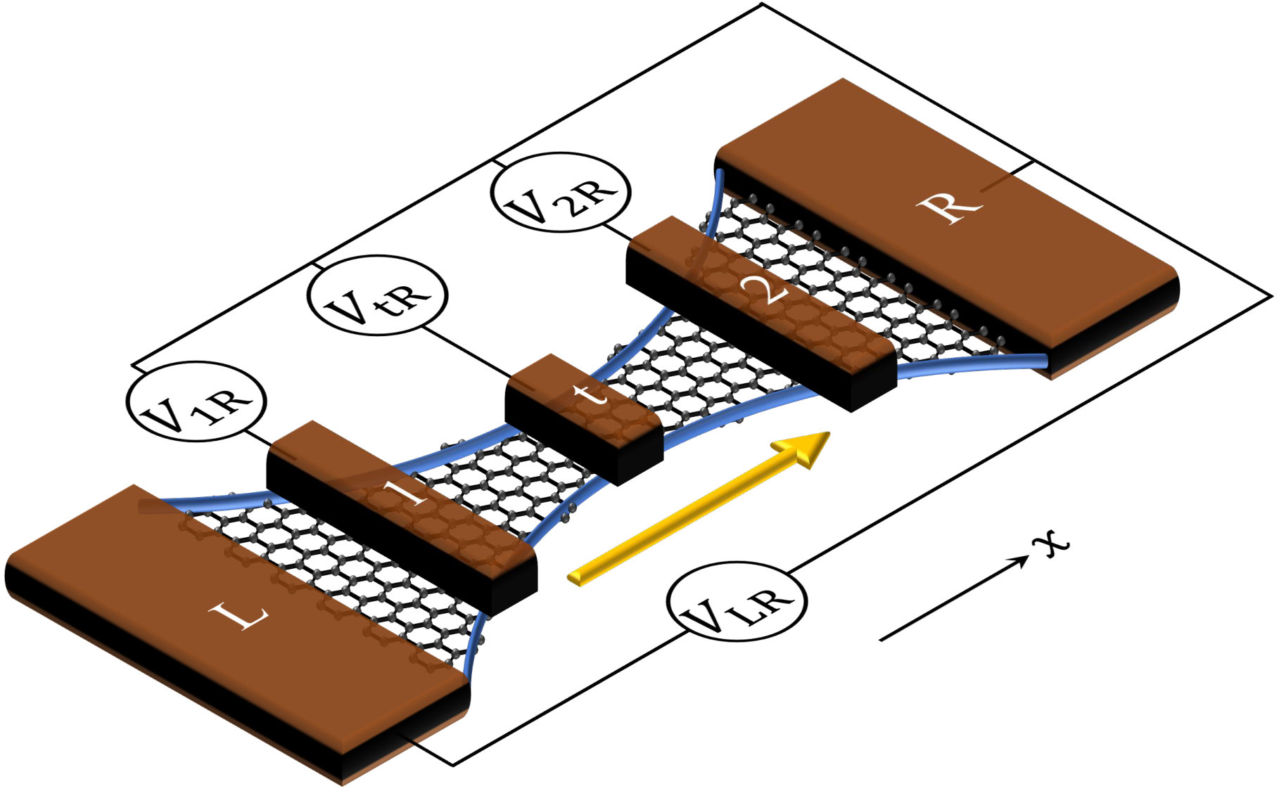 Figure 1
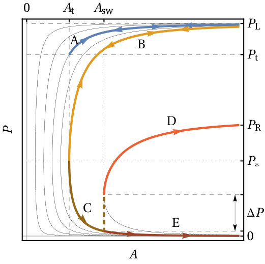 Figure 2
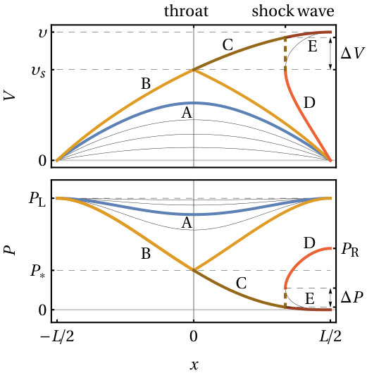 Figure 2
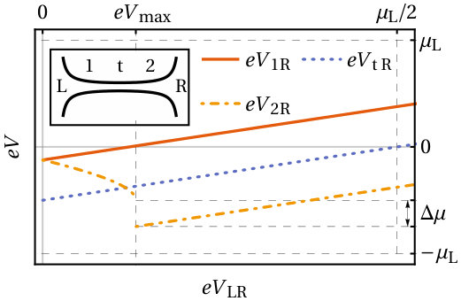 Figure 3
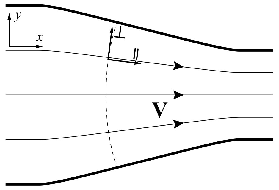 Figure 5
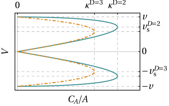 Figure 6
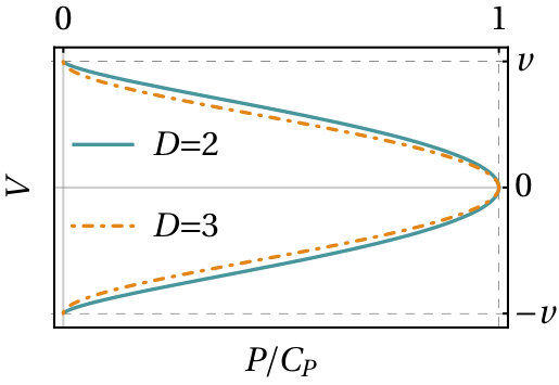 Figure 7
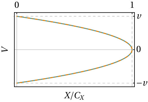 Figure 8
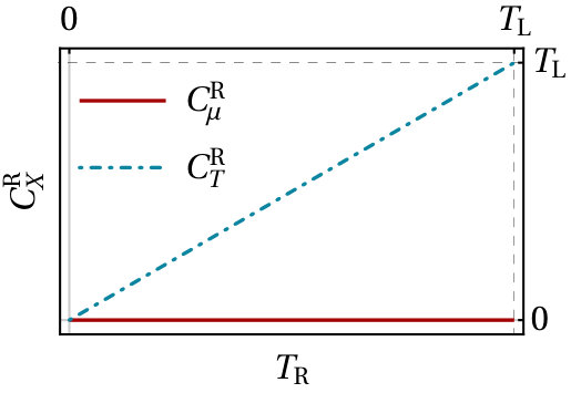 Figure 9
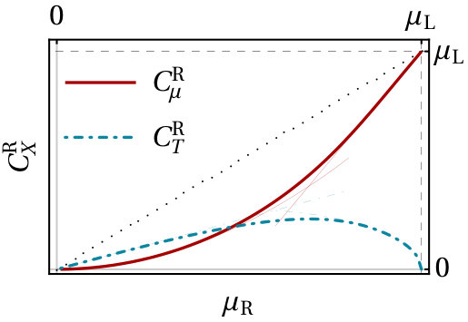 Figure 10
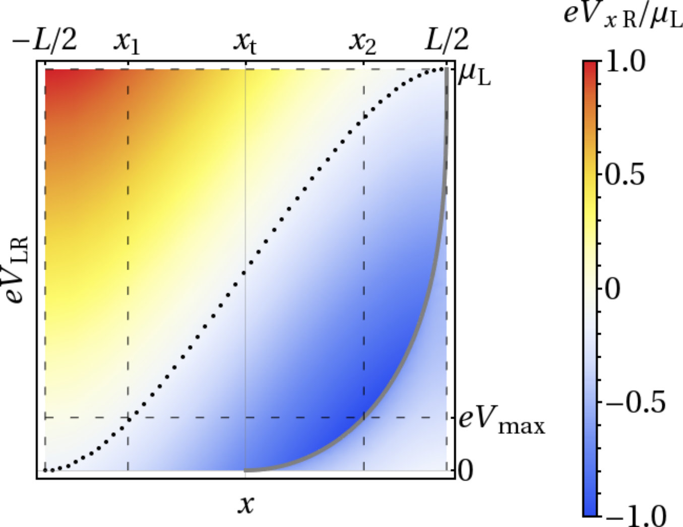 Figure 11
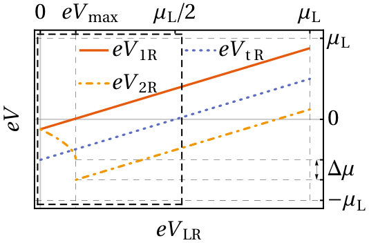 Figure 12
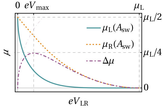 Figure 13
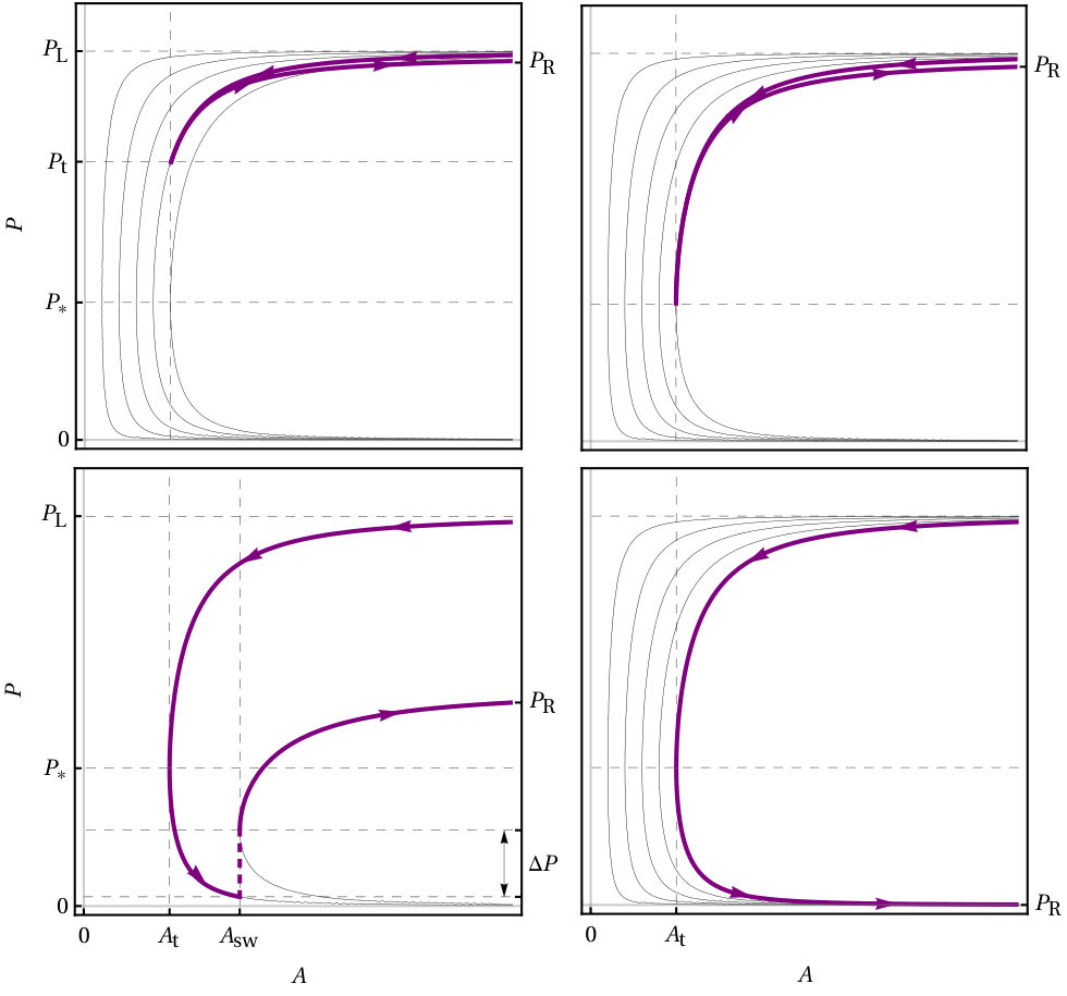 Figure 14
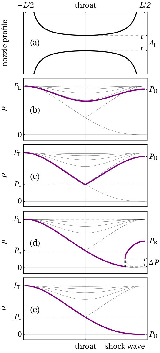 Figure 15
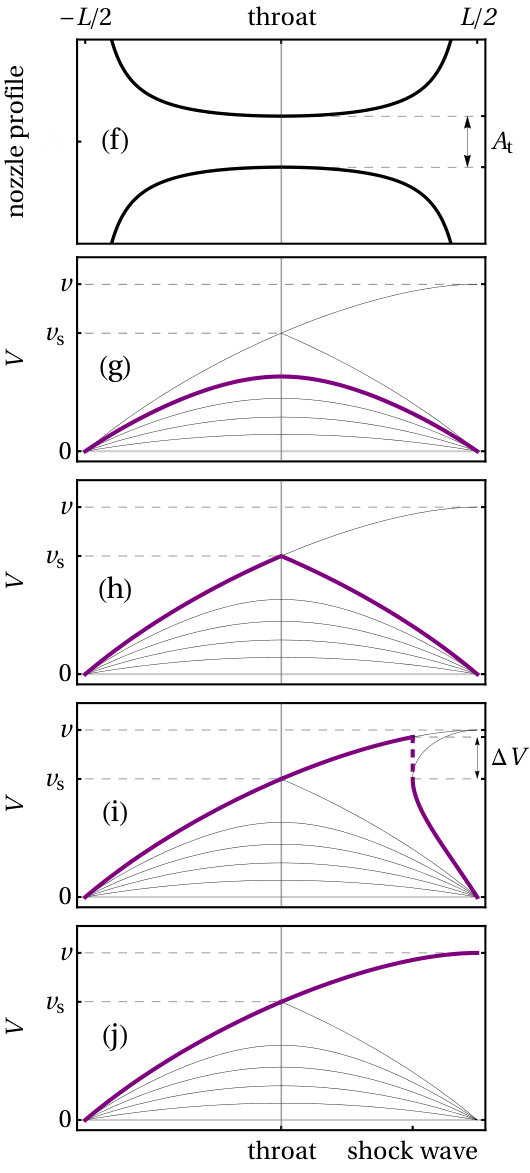 Figure 16
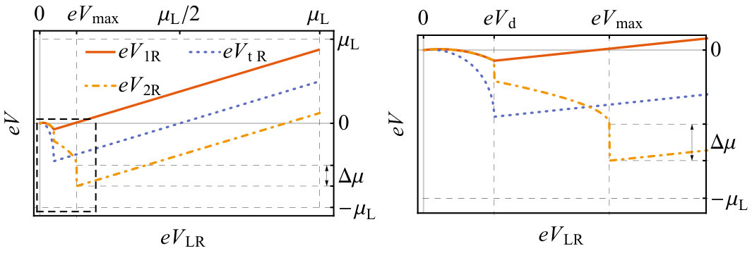 Figure 17
| Dirac Hamiltonian | number of spatial dimensions | ||
| Dirac velocity | speed of sound | ||
| momentum | vector of Pauli matrices | ||
|
chirality or nature of particle (electron or hole) with intensive thermodynamic conjugate
variable |
macroscopic energy density | ||
| interparticle scattering length | typical length scale of momentum relaxation | ||
| effective fluid mass density, with subscript 0 for vanishing flow velocity | particle number (density), with subscript 0 for vanishing flow velocity | ||
| particle current | charge of electron | ||
| pressure |
critical pressure (transition from subsonic to
supersonic flow) |
||
| pressure jump at shock front position | ratio of cross section of throat and cross section at certain position along nozzle | ||
| ratio of pressure drop versus pressure in left lead (where flow originates) | () | flow velocity (speed) | |
| cross section (or width) of nozzle profile | minimal cross section (throat of nozzle profile) | ||
| chemical potential | chemical potential difference (or voltage drop) at shock front position | ||
| temperature |
solution constant of the nozzle equation that
relates cross section to flow speed |
||
|
solution constants of the nozzle equations
representing chemical potential, temperature, and pressure for vanishing flow speed |
upper bound for | ||
| macroscopic momentum (energy flow) | electronic distribution function | ||
| Fermi-Dirac/hydrodynamic flow distribution function | polylogarithm functions | ||
| propagation direction of electrons | stress tensor | ||
| macroscopic chirality | chiral current | ||
| surface of a -dimensional sphere | typical interparticle collision time | ||
| typical time scale for momentum relaxation | viscosity | ||
| (dimensionless) viscosity parameter | electric field | ||
| magnetic field | bias voltage between left and right lead | ||
|
voltage difference between voltage probe with
label .. (position along nozzle) and right lead |
bias voltage with maximal voltage drop induced at the shock front | ||
| momentum relaxation-induced voltage difference across a nozzle | resistance |
Peer Reviews
No public reviews on file for this paper yet. If you reviewed it on a platform where reviews are public (OpenReview, ICLR, NeurIPS, ICML), you can paste yours below so the community can read it here.
Videos
No videos yet. Explain this paper in a talk, walkthrough, or lecture? Add one.
Taxonomy
TopicsQuantum Electrodynamics and Casimir Effect · Graphene research and applications · Radiation Therapy and Dosimetry
Supersonic flow and negative local resistance in hydrodynamic Dirac electron nozzles
Kristof Moors
University of Luxembourg, Physics and Materials Science Research Unit, Avenue de la Faïencerie 162a, L-1511 Luxembourg, Luxembourg
KU Leuven, Department of Physics and Astronomy, Institute for Theoretical Physics, Celestijnenlaan 200D, B-3001 Leuven, Belgium
Forschungszentrum Jülich, Peter Grünberg Institut (PGI-9), D-52425 Jülich, Germany
Oleksiy Kashuba
Universität Würzburg, Institut für Theoretische Physik und Astrophysik, Theoretische Physik IV, D-97074 Würzburg, Germany
Thomas L. Schmidt
University of Luxembourg, Physics and Materials Science Research Unit, Avenue de la Faïencerie 162a, L-1511 Luxembourg, Luxembourg
Abstract
In clean Dirac electron systems such as graphene, electron-electron interactions can dominate over other relaxation mechanisms such as phonon or impurity scattering. It has been predicted that in this limit, collective electron dynamics can be described by hydrodynamic equations. The prerequisites for electron liquids are already fulfilled in current experiments and hints of electron hydrodynamics have been identified in transport measurements. Here, we show that a nozzle geometry, implemented for example in a graphene sample, can cause a transition from subsonic to supersonic flow and provides an interesting probe for the hydrodynamic regime of Dirac electrons. In particular, we predict two distinct transport features that can be seen in the experimentally measurable voltage characteristics on the exit side of the nozzle: a pronounced negative local resistance, and an abrupt change of the electrostatic potential induced by an electron shock wave. Our results pave the way for an experimental identification of supersonic hydrodynamic electron flow and for the experimental study of electron shock waves.
Various electronic transport phenomena can be traced back to the propagation of individual charge carriers, in a ballistic or diffusive regime, for example. The description as individual carriers provides an extremely versatile framework, as the electrons in many condensed matter systems are well described as almost free quasiparticles. However, in recent years, a very different transport regime has taken center stage, namely hydrodynamic electron flow, which occurs in the opposite limit of very strong interparticle interactions [1]. Rather than relying on individual quasiparticles, modeling such transport is based on notions from the classical theory of hydrodynamics, such as the continuity equation and the Navier-Stokes equation. Hydrodynamic flow is possible irrespective of whether the underlying particles are fermionic [2, 3, 4] or bosonic [5, 6, 7, 8, 9, 10].
However, reaching the regime of hydrodynamic electron flow in experiments has proved difficult: in most materials deviations from purely ballistic transport are either caused by disorder-induced scattering (for instance, due to impurities) at low temperatures, or by electron-phonon scattering at higher temperatures. Both of these scattering mechanisms drive the system to a diffusive transport regime and thus inhibit hydrodynamic electron flow. Remarkably however, graphene has emerged as an ideal platform for reaching the hydrodynamic regime. In clean enough samples there exists a large temperature window where electron-electron interactions dominate over both disorder-induced scattering and electron-phonon interactions [11, 12, 1, 13]. In this temperature range, hydrodynamic flow with distinct transport signatures can be realized.
Several effects have already been proposed as signatures of hydrodynamic behavior: a negative nonlocal resistance due to vortex formation [14, 15, 16, 17, 18], a Poiseuille flow profile and the Gurzhi effect in the presence of boundaries [11, 19, 20, 21], superballistic transport [22, 23], as well as the Hall viscosity in the presence of a magnetic field [24, 25, 26, 27, 28, 29].
All the effects that are listed above appear in the regime of subsonic hydrodynamic flow. In this Article, we propose graphene tailored into a nozzle geometry as a feasible experimental setup for the investigation of the supersonic hydrodynamic regime. We predict that a so-called de Laval nozzle displays a number of electronic transport features which can be taken as strong indicators of supersonic hydrodynamic transport. In the perfect-fluid regime where the viscosity can be neglected, the major feature is an abrupt change of flow properties with the appearance of a shock front as the drift velocity increases from subsonic to supersonic speeds (the speed of sound of a two-dimensional hydrodynamic Dirac system is , where is the Dirac velocity).
In classical systems, a de Laval nozzle is widely used for steam turbines and rocket or jet engines and the underlying physics has numerous applications in other areas of physics. In particular, a relativistic de Laval nozzle provides a simple description of jets near black holes or neutron stars [30, 31]. In a condensed-matter context, such nozzle geometries have been considered for the realization of sonic black holes [32], e.g., in trapped Bose-Einstein condensates [33, 34, 35], with the analogue of an event horizon appearing where the flow enters the supersonic regime.
We will show that the properties of de Laval nozzles make them ideal for exploring the hydrodynamic behavior of Dirac electrons in condensed-matter systems, and that their realization with graphene is within reach with existing fabrication techniques and sample qualities. Hydrodynamic transport through a de Laval nozzle can give rise to supersonic flow with a shock front and very distinct voltage characteristics that do not depend on the details of the nozzle geometry. We also discuss the impact of viscosity and how the sharp shock front discontinuity in the flow profile turns into a continuous shock front remnant.
Nozzle equations
We apply the hydrodynamic equations that describe a strongly interacting electronic Dirac system in two or three spatial dimensions (see Methods section) to a system with a nozzle geometry, as shown in Fig. 1. The nozzle is characterized by a varying cross section (which has the dimension of length for the two-dimensional and of an area for the three-dimensional case) as a function of the nozzle coordinate , along which the flow is directed. We consider a smooth change of the nozzle cross section, i.e., , and we assume that the macroscopic quantities are uniform in the plane perpendicular to the flow direction. Note that the cross section in general refers to the effective cross section for the interior of the nozzle where the fluid flows freely without influence from the edges. Near the edges, the flow speed may be reduced due to friction [19], which would violate the assumption of uniformity perpendicular to the flow direction. Turbulent flow would also violate the uniformity assumption but is not expected in realistic samples in the regime dominated by electron-electron interactions. The Reynolds number of the nozzle can be estimated by , with the flow velocity, the typical length scale of the flow profile (i.e., the length of the nozzle in our case), the Dirac velocity, and the interparticle scattering length [1]. Turbulent flow is only expected for a Reynolds number of the order of or higher, requiring hydrodynamic transport over very large samples, which is typically prevented by momentum relaxation.
Under these assumptions, the flow profile is effectively one-dimensional [36] and the hydrodynamic equations simplify to:
[TABLE]
where , is the pressure, the flow velocity, the effective fluid mass density, and the particle density. The first equation is the stationary one-dimensional Navier-Stokes momentum equation in the nonviscous limit (). The last two equations are continuity equations that reflect the conservation of particle current and momentum , given by
[TABLE]
with , , and being functions of the nozzle coordinate . The electrical current is given by , and the energy flow by . This Article focuses on the velocity profile along the flow direction of the nozzle. This is notably different from previous works that focus mainly on the velocity profile perpendicular to the flow direction of highly viscous hydrodynamic Dirac systems with constrictions [22, 23, 20].
Starting from Eq. (1), we can express the change of flow speed and pressure with the nozzle cross section as
[TABLE]
where is the speed of sound (see Methods section). These relations essentially govern the flow through a nozzle and we therefore refer to them as the nozzle equations. Their derivation is provided in Sec. SII of the Supplementary Material (SM).
The nozzle equations tell us that, if the flow starts at subsonic speed , increases as the cross section decreases. This is a well-known consequence of Bernoulli’s law. However, as soon as exceeds , the behavior reverses and increases further with increasing cross section. This is the basic working principle of a de Laval nozzle: a section with decreasing cross section first accelerates the flow to the speed of sound, which is then attained at the throat of the nozzle (i.e., at the narrowest point with cross section ). Past the throat, an increasing cross section further accelerates the flow.
Solving for the flow speed as a function of the cross section with Eq. (3), we obtain
[TABLE]
with integration constant (assumed to be positive without loss of generality). This constant fixes the relation between flow speed and cross section and can, up to a prefactor (see Sec. SII B of the SM), be thought of as the total particle (or electrical) current that flows through the nozzle. Note that there is an upper bound for and, hence, also for the current, which can only be reached when at the throat. A solution for the pressure can also be obtained from Eq. (3) and is given by
[TABLE]
where we have introduced the constant , which corresponds to the pressure for vanishing flow speed.
Pressure-driven flow
To discuss the generic flow behavior of a Dirac electron fluid through a de Laval nozzle, it is convenient to consider a nozzle with length and nozzle coordinate , attached to infinitely wide leads, i.e., . Then, the possible boundary conditions for any flow profile are restricted to [see Eq. (4)], which is convenient to resolve the flow profile. We assume this geometry throughout the text but all our predictions remain qualitatively valid for nozzle profiles with cross sections of the leads much larger than that of the throat.
Stationary hydrodynamic flow is generally driven by a pressure gradient in the Navier-Stokes equation, as can be seen from the first equality in equation 1. However, every solution of the nozzle equations 3 with a flow speed that stays subsonic along the length of the nozzle leads to equal pressure at the entrance and the exit (Fig. 2, line A), where the flow speed vanishes and the pressure is given by in equation 5. The different subsonic flow profiles correspond to different values of or, equivalently, the current, with . As increases, the maximal flow speed, which is realized at the throat and equal to zero when , increases until it reaches the speed of sound when . This value of corresponds to the critical flow profile shown in Fig. 2 (line B), with the pressure dropping to the critical pressure at the throat and returning to the initial pressure at the nozzle entrance. As we will see below, a pressure gradient can be induced by a gradient of the chemical potential or temperature. Hence, in the subsonic regime, a finite current can flow with infinitesimal bias voltage or heat gradient, up to the maximal current that is proportional to the cross section of the throat and . When considering viscosity or momentum relaxation in realistic samples, there can be subsonic flow with finite pressure differences (bias voltages or heat gradients) between the leads and a smoother onset of supersonic flow is expected, as we discuss in Secs. SII D and SII E of the SM.
Apart from the critical flow profile, there is an alternative solution of equations 4 and 5 with , where the flow continues to accelerate, exceeding the speed of sound and reaching at the right lead, and the pressure dropping further past the throat (line C & E). The solution is referred to as the ideal flow profile and is realized when the pressure at the exit is equal to zero. We will see below that this requires the exit lead to be at zero temperature with chemical potential tuned precisely at the Dirac point, which is impossible to realize in practice.
Next, we consider two leads with different but finite pressures, denoted by for the left (right) lead, which necessarily induces a supersonic flow profile. Without loss of generality, we assume , keeping fixed, such that the flow always goes from left to right. Similar to the solution for ideal (supersonic) flow, the solution follows line B and C in Fig. 2. However, the flow needs to return to subsonic speeds to reach at the right lead, and this implies that the nozzle equations become singular at a certain position past the throat (see equation 3 with and ), corresponding to a line (for ) across the nozzle. Therefore, the values of and need not be the same to the left and right of this position. This allows us to match the seemingly incompatible solutions of equation 5, with for the solution that matches the pressure in the left (right) lead. To the left of the position where the nozzle equations become singular, we have , as for the critical and ideal flow profile. To the right, the value of follows from the conservation of momentum along the nozzle, yielding (see Sec. SII A in SM), which, in turn, yields . Having obtained and to the left and right of the singular point, one can see that there is a discontinuity in the flow speed and the pressure, as indicated by the dashed brown lines in Fig. 2. The latter reflects the appearance of a shock wave, which is a well-known phenomenon of supersonic hydrodynamic flows in de Laval nozzles [36].
The shock front appears to the right of the throat and its position along the nozzle can be obtained by first integrating the hydrodynamic equations over the infinitesimal interval , then inserting the solutions for the pressure and velocity of the left and right limits, and finally solving for the cross section of the shock front . The second equality in equation 1 yields , with denoting a jump of the macroscopic quantity across the discontinuity, and can be used together with the first equality to obtain . Inserting the expression for the pressure from the Methods section, we get the following condition for the discontinuity of the flow velocity:
[TABLE]
The numerical solution of this equation is given in Sec. SII A of SM. Starting from equal pressure and lowering the pressure in the right lead, a shock front appears near the throat and gradually shifts to the right lead, where it vanishes again. This is how the flow profile evolves from the critical to the ideal profile.
Note that the current flowing through the nozzle does not change for any supersonic profile in between the critical and ideal profile. The current and flow speed saturate at their maximum value at the throat when reaching the sonic barrier and remain constant as the pressure difference increases. Also note that the solution to the left of the shock front does not depend on the value of the pressure in the right lead. This is expected because the flow of information is bounded by the speed of sound of the Dirac fluid and, hence, the regions are causally disconnected. It is the position of the shock front itself that shifts when varying the pressure in the right lead, along with a change of the flow profile to its right. At the shock front, there is a pressure jump , which, in the case of , is maximal and equal to when , occurring at the position in the nozzle to the right of the throat where the cross section equals (see Sec. SII A in SM for details).
Voltage characteristics
So far, we have considered the flow through a nozzle in terms of the pressure, as in a conventional de Laval nozzle. However, since the temperatures and chemical potentials in the leads are the more accessible control parameters in electronic Dirac systems, we will study their effect on the flow profile in the following.
Based on explicit expressions for the particle number, mass density, and pressure in terms of the chemical potential, temperature, and flow speed of a hydrodynamic Dirac system, we obtain (see Sec. SII B in SM)
[TABLE]
where and are polylogarithm functions, is the temperature, and is the chemical potential. Rewriting equation 1 in terms of temperature and chemical potential, we obtain
[TABLE]
with solution given by
[TABLE]
where, similar to , the constants and represent the temperature and chemical potential, respectively, at vanishing flow speed.
We assume and low temperatures (), such that the flow is induced by a chemical potential difference, corresponding to a bias voltage (see Sec. SII B in SM for a more general treatment). Experimental signatures of hydrodynamic flow have already been reported in a regime where this assumption is appropriate [1].
From the explicit expression of the pressure in terms of the chemical potential in equation 8, it follows that in the low-temperature limit, such that a pressure gradient with supersonic flow from left to right is realized when . In this case, the flow profile inherits the temperature and chemical potential from the left lead, i.e., and . Unlike for the pressure, whose gradient directly drives the hydrodynamic flow, we cannot match the constants for temperature and chemical potential to the right of the shock front to their respective values in the right lead. The values of temperature and chemical potential downstream of the shock front can be obtained by making use of current and momentum conservation, yielding
[TABLE]
where is the Apéry constant. Note that, indeed, the chemical potential of the nozzle exit does not match with the right lead (), unlike for the pressure. Moreover, despite a low temperature in the leads, the exit temperature of the fluid, , is not necessarily small compared to . The hydrodynamic Dirac system heats up significantly while flowing through the nozzle, without any kind of dissipation [37].
The resulting local voltage with respect to the right lead , which can also be understood as a local resistance , is shown in Fig. 3 as a function of the bias voltage, while keeping fixed, for three positions along the nozzle. As illustrated in the inset and on Fig. 1, we consider positions to the left, to the right, and at the throat. The three profiles display a negative local voltage (i.e., with opposite sign as compared to the bias voltage) or, equivalently, negative local resistance that is more pronounced for the position closest to the exit. In addition, there is a discontinuous change of the local voltage as a function of the bias voltage to the right of the throat. This is a consequence of the shock front moving through the nozzle (past the throat) and is an indirect signature of the shock wave of the hydrodynamic Dirac system showing up at that position. The magnitude of the discontinuity (see Fig. 3) on the bias voltage and is maximal and approximately equal to when , which follows from the full numerical solution of (see Sec. SII C in SM). The maximal voltage drop shows up where the cross section is approximately equal to , being the cross section where positions 1 and 2 are considered in Fig. 3.
Discussion
Since we consider hydrodynamic flow without momentum relaxation, any finite bias voltage or pressure difference induces a supersonic flow profile. A smoother onset of supersonic flow is expected in the presence of weak momentum relaxation, with the subsonic-to-supersonic transition in Fig. 2 now appearing at nonzero pressure difference. This also affects the local voltage profile of Fig. 3, but the signatures of supersonic flow survive as long as momentum relaxation is sufficiently weak over the length of the nozzle. Details on the impact of weak but finite momentum relaxation are provided in Sec. SII D of the SM.
In the case of strong momentum relaxation, the (supersonic) hydrodynamic transport behavior is lost and one can expect the nozzle to behave as an Ohmic resistor, with the local voltage profile scaling linearly as a function of the bias voltage and its slope depending on the position along the nozzle and the details of the nozzle geometry. In this regime, neither a negative local resistance nor a discontinuity in the local voltage profile are expected. A simple first step in identifying the hydrodynamic regime of the nozzle with supersonic flow would be to measure the current as a function of the bias voltage. There should be a clear transition from an Ohmic linear increase to a constant, as the current in the supersonic flow regime is fixed. For a graphene nozzle with a wide throat and an electron density on the order of , the saturation current of supersonic flow will be in the range of a few .
If the length of the nozzle does not significantly exceed the interparticle scattering length, a ballistic instead of a hydrodynamic transport regime is expected. The distinct transport signatures of a nozzle with supersonic hydrodynamic flow will also not appear in this regime because of the following reasons. First, we predict a negative local resistance past the nozzle throat, along the direction of the injected current and overall bias voltage drop, and becoming more pronounced further away from the current source, up to the position of the shock front. This is opposite to the behavior in Ref. [18], in which the authors show that a negative nonlocal resistance can be obtained in the ballistic regime when a current originates from a narrow source. Second, the cross section variations of the nozzle are smooth and, therefore, a standard ballistic treatment of a nozzle geometry, based on the transfer-matrix method, for example, will naturally yield a gradually decreasing voltage profile, with neither negative local resistance nor discontinuity in the local voltage profile. Lastly, we present a consistent picture of negative local resistance and discontinuity in the local voltage profile, based on hydrodynamic transport with supersonic flow. To the best of our knowledge, there is no ballistic transport analysis that can similarly reproduce both features.
We have assumed throughout this text that the Dirac electron fluid is nonviscous while, in real nozzle samples, the interparticle scattering length is finite and the fluid therefore viscous [38]. A finite viscosity corresponds to the consideration of a finite interparticle scattering length when deriving the hydrodynamic equations from the quantum kinetic equation (see Sec. SI of our SM), giving rise to a viscosity term in the Navier-Stokes equation [1]. In Sec. II A of the SM, we discuss the impact of viscosity on the nozzle equations and the resulting flow profiles in detail. In general, we find that an effective viscosity parameter governs the corrections to the 1D flow profiles, and these corrections become very small when the interparticle scattering length of the Dirac electrons is small compared to the dimensions of the nozzle. In this regime, there is excellent quantitative agreement between the viscous flow profiles (with low effective viscosity) and the nonviscous flow profiles (obtained in the perfect-fluid regime). The discontinuity in the flow profile turns into a continuous shock front remnant with a highly peaked deceleration of the flow speed, i.e., a steep drop of the flow speed, and, correspondingly, a steep upturn of the pressure. Hence, a steep (albeit continuous) drop of the local voltage as a function of the bias voltage (as shown in Fig. 3) is expected past the throat when the shock front remnant passes the voltage probe and the effective viscosity is sufficiently low.
The realization of supersonic flow in graphene should be within reach with existing fabrication techniques and sample qualities. Large drift velocities () and low electron densities, , have already been reported [39, 40, 1]. The nozzle geometry itself should induce a further increase in velocity so seems to be within reach. To resolve the local current and voltage profile of a graphene nozzle, a recently developed noninvasive technique based on a cantilevered probe could be employed [41, 21]. Apart from graphene, a Dirac de Laval-nozzle and its phenomenology can also be considered for other condensed matter systems with ( or ) Dirac fermions, with the surface states of a 3D topological insulator and Dirac or Weyl semimetals as notable examples [42, 43].
It has been shown that a sonic analogue of a black hole can be realized with a supersonic fluid, with the region where the fluid turns supersonic representing the event horizon [44]. The spread of information is bounded by the speed of sound in place of the speed of light in this hydrodynamic system. For a supersonic de Laval nozzle as considered here, it is expected that quantized density waves or phonons of the hydrodynamic Dirac system are emitted from the throat of a supersonic nozzle toward the entrance with a black body spectrum, analogous to Hawking radiation forming near the event horizon of a black hole [32]. The Hawking temperature of this spectrum can be obtained from the flow speed through T_{\textrm{H}}=\bigl{.}\hbar\partial(|V|-v_{\textrm{s}})/(2\pi k_{\mathrm{B}})\bigr{|}_{|V|=v_{\textrm{s}}}=\hbar v/(2\pi k_{\mathrm{B}}L), with the last step obtained for the width profile considered in Fig. 2. The expression yields a temperature of the order of for a graphene nozzle with length in the range, comparable to the temperature of black hole analogues based on hydrodynamic flow of microcavity polaritons [45]. It is the equivalent of a black hole with a mass one thousand times smaller than the mass of the earth. While being two orders of magnitude lower than the typical temperature that is required in graphene to realize hydrodynamic transport, this Hawking temperature is rather high when compared to other condensed-matter systems that have been proposed, such as superfluid helium or Bose-Einstein condensates, only yielding temperatures in the K [46] or nK [33] range. Detection of this Hawking radiation can be envisioned with a very sensitive voltage probe that identifies the voltage fluctuations due to fluctuations in the fluid of Dirac electrons, and cross-correlating the fluctuations on opposite sides of the shock front would be able to disentangle the Hawking radiation from intrinsic temperature-induced fluctuations. A high ratio of Hawking temperature versus the temperature of the Dirac electrons is crucial. This is challenging, as lowering the temperature of the Dirac electrons will increase the interparticle collision length (typically, ), in turn limiting the minimal size of the nozzle and the maximal Hawking temperature that can be achieved. Whether it could be observed in a given hydrodynamic Dirac system will ultimately depend on the details of the Dirac spectrum and the different scattering processes in that system (interparticle and momentum relaxing).
In conclusion, we have considered a de Laval nozzle to study the hydrodynamic behavior of strongly interacting Dirac fermions in condensed-matter systems. Applying a bias voltage to two leads at opposite ends of the nozzle, a supersonic hydrodynamic flow profile with a shock wave can be induced, as obtained from the Euler equations for the hydrodynamic Dirac system. The flow profile is driven by a pressure gradient between the two leads, which can be obtained from temperature or chemical potential gradients. This results in a distinct voltage profile, which can be probed by locally resolving the voltage profile along the nozzle while sweeping the bias voltage. Our findings provide two interesting signatures: a region of pronounced negative local resistance in the low-temperature regime with respect to the lead where the flow is directed, and a discontinuity in the voltage profile. This discontinuity is a signature of a shock wave of a hydrodynamic Dirac system, which is a distinctive signature of supersonic hydrodynamic flow.
Methods
Hydrodynamic equations in Dirac systems
We consider massless Dirac fermions with the kinetic Hamiltonian in spatial dimension or (in units with ), where is the Dirac velocity. For , is the vector of Pauli matrices, and is the momentum (defined analogously for ).
In the limit of strong interparticle interactions (with the particles being Dirac electrons or holes), other interactions can be neglected (e.g., with impurities or phonons) and this system can be described by the momentum-conserving hydrodynamic equations of a nonviscous fluid [31, 1]. While commonly described as a viscous fluid, a hydrodynamic Dirac electron system can be described as a nonviscous fluid when expanding the hydrodynamic equations as a function of , with the typical interparticle scattering length and the typical length scale of the flow profile (i.e., the length of the nozzle in our case), and only keeping the zeroth order terms. This approximation is suitable for resolving the flow profile on length scales much larger than the interparticle scattering length and allows us to solve the hydrodynamic equations in the nozzle analytically (see Sec. SII E in SM for comparison with viscous flow across the nozzle). Furthermore, momentum-conserving hydrodynamic flow implies that is smaller than the typical length scale for momentum relaxation , induced for example by collisions with impurities or phonons. It is therefore essential that the design of the nozzle satisfies the constraints , provided that such a window with hydrodynamic transport exists. For a very clean graphene sample at around , should be of the order of [1].
Under these assumptions, it is possible to define macroscopic quantities such as the charge density , (effective fluid) mass density , energy density , hydrodynamic pressure , as well as the flow velocity that satisfy the hydrodynamic Euler equations,
[TABLE]
Their precise definitions and derivation from the quantum kinetic equation can be found in Sec. SI of our SM. These Euler equations are, respectively, manifestations of the momentum, energy, and particle number conservation laws respected by the electron-electron interactions in the stationary (zero-frequency) regime (see Refs. [47, 48] for recent work on high-frequency hydrodynamic transport with plasmonic effects). The relation between the mass density and the pressure for our relativistic system is
[TABLE]
where , and the last equality relates the pressure to the energy density. A well-known result from relativistic hydrodynamics states that the speed of sound of a -dimensional Dirac system is equal to [31], so supersonic flow corresponds to .
Acknowledgements
K.M. and T.L.S. acknowledge the support by the National Research Fund Luxembourg with ATTRACT Grant No. 7556175, O.K. acknowledges the financial support from SFB1170, “ToCoTronics”, and K.M. acknowledges the financial support by the Bavarian Ministry of Economic Affairs, Regional Development and Energy within Bavaria’s High-Tech Agenda Project “Bausteine für das Quantencomputing auf Basis topologischer Materialien mit experimentellen und theoretischen Ansätzen” (grant allocation no. 07 02/686 58/1/21 1/22 2/23).
SI Macroscopic quantities & Hydrodynamic equations of Dirac systems
The hydrodynamic description of a -dimensional ( or ) Dirac system is based on the following macroscopic quantities: the particle number , the current , the macroscopic momentum , macroscopic energy , and the stress tensor . They are defined as a function of the (semiclassical) electron distribution function as follows (in units with ):
[TABLE]
where is the Dirac velocity, is the momentum () and the electron or hole nature of the state or, equivalently, its chirality, such that a state with momentum and chirality has an energy . Moreover, is a unit vector in the direction of the momentum. In this Article, we consider a stationary flow, in which case all macroscopic quantities will depend only on position and not on time. In addition, we will consider the macroscopic chirality and the chiral current , given by
[TABLE]
We consider a Dirac system subject to interparticle collisions that conserve the total particle number, chirality, momentum and energy, which can be represented by their intensive thermodynamic conjugate variables , , , and , respectively. The system can then be represented by a distribution function , which cannot be affected by the interparticle collisions and can be expressed in terms of the Fermi-Dirac distribution . We refer to as the hydrodynamic flow distribution function, and proceed with the natural redefinition of in terms of the flow velocity , of in terms of temperature , of in terms of the chemical potential , and of in terms of a chirality-dependent shift of the chemical potential and (in units with ). The particle number , for example, can be obtained from straightforward integration of the Fermi-Dirac distribution function as follows:
[TABLE]
with gamma function , polylogarithm functions , and where we have made use of the relation and redefined to render the integral finite. The surface of a -dimensional sphere and the function were also introduced, defined as:
[TABLE]
We can confirm this result by exploiting Lorentz invariance. We consider a Lorentz boosted reference frame with boost speed and momentum , related to as follows:
[TABLE]
with , and () the component(s) of the momentum parallel (perpendicular) to the boost direction. The last equation presents the Lorentz invariant integration measure over all momenta. This can be used to obtain
[TABLE]
where we have considered a boosted reference frame along the flow, in opposite directions for both terms.
Having obtained the other macroscopic quantities in a similar manner, one can verify that the following relations hold:
[TABLE]
We have added a subscript ’H’ to the (chiral) current and the stress tensor, as these quantities are obtained from the hydrodynamic flow distribution function but are not conserved by interparticle collisions. The relation between the energy and the trace of the stress tensor is valid in general, however. Note that we have introduced the pressure as the component of the stress tensor for vanishing flow velocity, which can be shown to agree with the thermodynamic definition as the derivative of the energy with respect to the system volume for constant entropy and particle number [1]. We have also introduced the effective fluid mass density that relates the flow velocity to the macrosopic momentum. It can be obtained in a similar manner as the particle number, yielding
[TABLE]
It is the analog of the mass density of a conventional fluid.
In the Main Text, we do not consider chiral symmetry breaking, which would correspond to . This quantity only appears inside the functions , which can be expanded for small as:
[TABLE]
Hence, we have only considered the leading-order contribution. This chiral symmetry is equivalent to considering an electron-hole-symmetric system, with the distribution for electrons and holes identical to each other upon changing the sign for energy and momentum.
Approximations for the macroscopic quantities can be obtained in the low and high temperature regimes, by making use of the following expansions:
[TABLE]
Here , with the definition of Eq. (S5), and , with , , , and , for example. Note that a separate treatment is required for and as . For the particle number and effective fluid mass density, for example, we obtain the following limits in two and three spatial dimensions:
[TABLE]
The dynamics of the macroscopic quantities can be obtained from the semiclassical Boltzmann equation, which incorporates the scattering mechanisms through the collision integral [2]. We only consider the regime in which the interparticle (-) collisions are dominant, neglecting any other scattering mechanism:
[TABLE]
with drift term due to external electric and magnetic fields, and , respectively, and collision integral . From this equation, we obtain the following hydrodynamic equations for the particle number, chirality, momentum and energy, noting that the right-hand side vanishes for these quantities:
[TABLE]
where it is understood that the divergence on the third line acts on the first index of the stress tensor. Note that the flow of energy is proportional to the momentum in the absence of an electric field. They are related by a factor of , as can be seen from Eq. (S22).
Close to a hydrodynamic flow distribution, one can write and , with small corrections and . The corrections can be obtained from the Boltzmann equation, linearized around the hydrodynamic flow distribution. We further assume the relaxation time approximation with collisions characterized by a single interparticle collision time (the Callaway ansatz [3, 4, 5]), yielding:
[TABLE]
with distribution function . From this equation, it is clear that the corrections to the Fermi-Dirac values vanish in the nonviscous-fluid limit for infinitely strong interparticle collisions. It is important to note that the gradient terms vanish if is a position-independent function of the quantities. In this work, we mainly consider a space-dependent distribution function whose distribution is captured by local conjugate variables, according to the zeroth order approximation [6, 1], being a suitable ansatz for resolving a flow profile that varies over length scales much larger than the interparticle scattering length.
In the stationary regime and in the absence of electric and magnetic fields, the hydrodynamic equations for particle number, momentum and energy that follow from these considerations are given by:
[TABLE]
Inserting the Fermi-Dirac relations of Eq. (S9), we obtain precisely the hydrodynamic equations of Eq. (13) in the Main Text. We can safely neglect the electric and magnetic fields as very low electron densities are required to reach the hydrodynamic regime in Dirac electron systems, and thus the self-generated fields of the density (gradients) and currents of electrical charge will also be very small.
The speed of sound can easily be obtained from linearizing Eqs. (S21) and (S22) around a fluid at rest () with , , . We obtain
[TABLE]
The equations can be combined to form a wave equation
[TABLE]
if one takes into account the definition of the sound velocity as .
SII Dirac electron nozzle
We apply the hydrodynamic equations of Eq. (S24) to resolve the velocity profile of a nozzle geometry (see Supplementary Fig. S1). We rewrite the velocity with unit vector and we can write , such that the relations in Eq. (13) of the Main Text become:
[TABLE]
with the last line valid for any unit vector . The divergence of the normalized flow vector is related to the increase or decrease of the cross section of the nozzle by
[TABLE]
assuming laminar flow and thereby ruling out turbulent flow. Inserting this into Eqs. (S28) and (S29) and adding Eq. (S30), we retrieve the nozzle equations in (1) of the Main Text, where the subscript of the partial derivative, indicating that it acts along the direction of the flow, is omitted. The last equation derived here, Eq. (S31), describes how a flow profile makes corners and does not affect the nozzle effect. Moreover, it is irrelevant for a straight nozzle geometry with small deviations of the cross section, rendering the flow profile effectively one-dimensional (along the direction of ).
Now we can relate the cross section to the flow speed. Combining the first and second equality of Eq. (1) of the Main Text, we obtain:
[TABLE]
As in the Main Text, we omit the subscript of the partial derivative. Combining the last equality of Eq. (1) of the Main Text with the expression for the pressure in Eq. (S9), we get:
[TABLE]
These equations can be combined to obtain Eq. (3) of the Main Text.
To derive the nozzle equations in terms of temperature and chemical potential [Eq. (9) in Main Text], some additional manipulations are required. Let us separate the velocity dependence,
[TABLE]
where we define and . These definitions can be used to rewrite Eq. (S33) as follows:
[TABLE]
Let us parameterize and as functions of the temperature and its ratio with chemical potential :
[TABLE]
Then Eqs. (S37) and (S38) transform into
[TABLE]
which immediately gives
[TABLE]
The solution of Eq. (S36) is
[TABLE]
with an integration constant that fixes the relation between the cross section of the nozzle and the flow speed. Note that there is an upper limit for , namely,
[TABLE]
The solutions are presented in Supplementary Fig. S2a. The solution of Eq. (S42) is given by
[TABLE]
with the chemical potential and temperature for vanishing flow speed (see Supplementary Fig. S2c). The formulae for and have the same form. We can get the dependence on cross section by substituting Eq. (S45) in Eq. (S43), resulting in
[TABLE]
and an identical equation for . The hydrodynamic equations in principle cannot match the chemical potential and temperature at the entrance and exit of the nozzle with the values in the leads. In the motionless case, i.e., , the chemical potential and can be coordinate-dependent, but if the pressure [equal to for ] is constant, the flow gradient is zero and the hydrodynamic Navier-Stokes equation does not induce any flow. Thus, we should always match the pressure of the leads and cannot match both and .
A Pressure
An explicit expression for the pressure in terms of temperature, chemical potential and flow speed can be obtained from Eq. (S10) and the relation for the pressure in Eq. (S9), resulting in:
[TABLE]
where the last line is obtained with Eq. (S45) and is given by:
[TABLE]
which can be interpreted as the pressure for vanishing flow speed, in analogy to and being the chemical potential and temperature for vanishing flow speed, respectively. The relation is presented for and in Supplementary Fig. S2b. The pressure can also be related to the cross section by combining Eq. (S43) with Eq. (S47):
[TABLE]
as presented in the Main Text in Eq. (5).
The momentum is conserved throughout the nozzle identical for any position along the nozzle and given by:
[TABLE]
where the last equality is obtained by making use of Eqs. (S43) and (S47). The same conservation law applies to the energy flow . Thus, we obtain the following relation:
[TABLE]
with pressures and for the left and right lead, respectively, and the superscript denoting whether the constant belongs to the solution to the left or to the right of the shock front (see discussion of supersonic flow profile in Main Text). Combining this relation with Eq. (S49) and the expression for in case of a supersonic flow profile from left to right, i.e., (with minimal cross section at the throat of the nozzle) we obtain the following relation between the cross section and the pressure of the nozzle:
[TABLE]
To determine the position of the shock front and its cross section , we infinitesimally integrate Eq. (1) of the Main Text across the discontinuity. The integration of the second equality gives
[TABLE]
which tells us that is conserved across the discontinuity. That property can be used in the integration of the first equality, yielding
[TABLE]
Inserting the relation for the pressure of Eq. (S9), we get:
[TABLE]
We proceed to solve this equation for a Dirac system in two spatial dimensions (). Making use of Eq. (S49), we can express the flow speeds just in front and past the jump in terms of the cross section of the throat and the shock front, and the pressure in the leads:
[TABLE]
with critical pressure and with . The flow speed (pressure) is supersonic (subcritical) on the left side of the shock front and subsonic (supercritical) on the right. Inserting the flow speeds in Eq. (S56), we can relate the ratio of pressures in the leads to the ratio of cross sections for the throat and the shock front, leading to the following relation:
[TABLE]
The last factor in the equality is approximately equal to one such that , with a deviation of at most 15% (see Supplementary Fig. S3). We can write
[TABLE]
with written explicitly in Eq. (S59) and obtained by solving the equation for instead. These functions are shown in Supplementary Fig. S3. The pressure at the shock front has a jump , which can be obtained explicitly from Eqs. (S58) and (S59). If we fix and vary , the maximal pressure jump is given by the maximum of the function , which leads to the following values for the cross section of the shock front, the pressure in the right lead, and the size of the pressure jump:
[TABLE]
An example of a supersonic flow profile with finite pressure difference and discontinuity in pressure and flow velocity at the shock front position is presented in Fig. 2 in the Main Text.
B Chemical potential and temperature
We have seen that, to obtain a flow from left to right, we need . In terms of the temperature and chemical potential, we can see from Eq. (S48) that this translates to the following condition:
[TABLE]
An equal pressure is obtained when the left-hand side is equal to one, as required for a subsonic flow profile. In the high and low temperature regimes of the leads, and , respectively, the condition simplifies to and , making use of the expansion in Eq. (S12). As expected, the gradient of the temperature (chemical potential) determines the direction of the flow in the regime where the temperature (chemical potential) dominates, with the flow going from high to low temperature (chemical potential).
To resolve the constants for the chemical potential and temperature profiles that correspond to the solution of the nozzle equations, and , we need another relation in addition to Eq. (S51), originating from momentum (or equivalently, energy flow) conservation. We make use of the conservation of particle current , which is equal to:
[TABLE]
making use of Eqs. (S1), (S43) and (S45). As for the momentum flow, we obtain the last equality from considering an infinitely wide lead with . It is tempting to interpret in this expression as the temperature and chemical potential in the left (right) lead, but this is incorrect, as the flow at the exit does not automatically match the temperature and chemical potential of the lead. Only the pressure in both leads should be matched in general, as governed directly by the Navier-Stokes equation. The integration constants for temperature and chemical potential inherit the values from the lead where the flow originates, whereas, at the exit, they follow from the conservation of current and momentum along the nozzle.
Let us consider a flow that goes from left to right now and work out the flow profile and corresponding profiles for the chemical potential and temperature. In this case, we have , and the following relations hold:
[TABLE]
which follow from matching the current and the momentum in both leads and from matching the pressure in the right lead, respectively, making use of Eqs. (S48), (S50) and (S63). We separate the cases of subsonic and supersonic flow:
[TABLE]
These relations are sufficient to extract the values of and reconstruct the profiles in the nozzle via Eq. (S46).
We proceed here by considering explicitly the case of . The solution of Eq. (S46) is then given by:
[TABLE]
and an identical solution holds for . In the subsonic regime, we get the following profile in the nozzle
[TABLE]
with related to the current via Eq. (S67). In the supersonic regime, the profile to the left of the shock front is given by:
[TABLE]
where the () sign corresponds to the solution to the left (right) of the throat. Past the shock front, we get:
[TABLE]
To solve for the values of and and the resulting profile past the shock front, we can use the two independent equations that remain from Eqs. (S64)-(S66):
[TABLE]
making use of the relation between and in the supersonic regime, given by Eq. (S68). Let us consider first the limit regime . Then we have:
[TABLE]
We see that the exit temperature matches the value in the right lead, whereas the chemical potential does not (see Fig. S4a). For the opposite limit regime, with , we obtain:
[TABLE]
In this case, a small exit temperature, , is not guaranteed. In the limit of very small chemical potential difference, , we can expand the left-hand side of both equations, using the expansions in Eqs. (S12) and (S13), yielding:
[TABLE]
In the opposite limit, , we can consider the following expansion and corresponding solution:
[TABLE]
The general solution of Eq. (S77) for the low entrance-temperature regime is shown in Supplementary Fig. S4b, together with the asymptotes obtained in Eqs. (S78) and (S79). Note that there is significant hydrodynamic heating in general, with the exit temperature being proportional to the chemical potential in the entrance lead, which is considered to be much larger than the temperature in the leads. Only when does the chemical potential at the nozzle exit match with the right lead. The case is impossible in real experiment since it automatically forbids a nonzero charge current in the right lead.
C Voltage characteristics
Based on the results of the previous section, we can reconstruct the voltage profile for a de Laval nozzle of Dirac electrons connected to two leads with a bias voltage . In the low-temperature regime (), the bias voltage is related to the chemical potentials in the leads as follows:
[TABLE]
When momentum relaxation and viscosity can be neglected, any finite voltage difference will automatically induce a supersonic flow profile and we can use the relations of Eq. (S68) to obtain:
[TABLE]
The solution constants for temperature and chemical potential follow from Eqs. (S64)-(S66). In the case of , we can use the solution of Eq. (S77) and obtain the profile of the chemical potential at any position along the nozzle . In this way, we can define the local voltage with respect to the right lead as (see Figs. S5a and S5b). Note that we can equivalently consider a nozzle resistance and a local resistance (with respect to the right lead) without ambiguity, as the current remains constant (equal to ) for any finite bias voltage.
Similar to a discontinuity of flow speed and pressure at the shock front position, there is a discontinuity of the chemical potential or, equivalently, the local voltage profile. The chemical potential jump at the shock front can be obtained by combining Eqs. (S48), (S59), (S68), and (S72)-(S73), yielding
[TABLE]
The result is shown as a function of the bias voltage in Supplementary Fig. S5c. The bias voltage that induces a maximal voltage drop at the shock front, denoted by , can be extracted from the numerical solution for of Eq. (S77), which leads to with a drop of . For this bias voltage, the shock front appears to the right of the throat where the cross section of the nozzle is approximately equal to , as can be obtained from the following relation for the cross section of the shock front as a function of the chemical potential in the leads:
[TABLE]
This cross section is slightly larger than the one with maximal pressure jump (with cross section approximately equal to , as obtained in Sec. A).
D Momentum relaxation
A pressure difference for a subsonic laminar flow profile can be described with an effective momentum relaxation term in the 1D Navier-Stokes equation [see Eq. (13) in Main Text]:
[TABLE]
describing dissipative scattering processes in the system, due to impurity or phonon scattering for example, with a phenomenological momentum relaxation time . For weak dissipation, i.e., , the pressure is weakly affected, so its correction as a function of the nozzle coordinate, , can be calculated as:
[TABLE]
having made use of Eq. (S50). Here we assumed that the nozzle starts at and ends at , with , and consider explicitly the nozzle profile (as for Figs. 2b and 2c in the Main Text) to obtain the last equality. The total pressure difference between the two leads due to momentum relaxation is thus given by:
[TABLE]
again considering the nozzle profile to obtain the last equality. From this result, it is clear that momentum relaxation gives rise to a smoother onset of supersonic flow, as a subsonic flow profile already undergoes a small pressure decrease due to momentum relaxation. A finite minimum pressure difference is thus required to reach the supersonic flow regime. The transition to supersonic flow is presented in Figs. S6 and S7.
Let us now look at how the momentum relaxation term affects the chemical potential profile at the throat () and to its left () and right (), where the cross section is equal to (similar to Fig. 3 in the Main Text). We introduce a chemical potential that corresponds to the value of that induces a critical flow profile in the presence of momentum relaxation. Associated with this, there is a momentum relaxation-induced voltage and a momentum relaxation-induced resistance . We further assume .
For , we are in the subsonic regime with current equal to and we make use of Eqs. (S67) and (S71) to obtain:
[TABLE]
In the supersonic regime, the current is equal to and is given by:
[TABLE]
where . In order to probe the discontinuity at the shock front, it is clear that momentum relaxation needs to be sufficiently weak such that . Summarizing the results, we get:
[TABLE]
The results are illustrated in Supplementary Fig. S8.
E Viscosity
In this section, we consider the impact of (bulk) viscosity on the (supersonic) flow profiles in a Dirac electron nozzle. The viscosity can be described as an additional term in the Navier-Stokes equation, given by , with constant (bulk) viscosity [7]. Under the assumption of laminar flow, in which case the transverse component of the Laplacian of the viscosity term drops out () and the flow equation remains one-dimensional, viscous flow across the nozzle can be described with the following modified 1D Navier-Stokes equation [see Eq. (13) in Main Text]:
[TABLE]
with viscosity .
With the viscosity term included, the 1D nozzle equation becomes:
[TABLE]
writing the viscosity term in terms of an effective viscosity . Note that considering this effective viscosity to be constant is equivalent to considering the physical viscosity to be constant due to the conservation of momentum (). This assumption thus boils down to neglecting any dependence of the viscosity on chemical potential and temperature (also see subsection on viscosity in graphene below), which vary across the nozzle in general. Further note that the is dimensionless for a two-dimensional () nozzle, e.g., a graphene-based nozzle.
We numerically resolve Eq. (S92) throughout the nozzle region, starting with boundary conditions for () and at the left lead. In practice, we propagate the solution from a very small but finite distance from the infinitely-wide left lead with different (finite) flow speeds and . The acceleration of the flow readjusts to the proper boundary value over a very short distance and well-behaved subsonic and supersonic flow profiles are obtained, as can be seen in Fig. S9.
E.1 Pressure-driven flow
In the section above, we have managed to obtain the flow profile for a given initial flow speed at the left lead and a particular value of effective viscosity . Here, we work out how the viscous flow profile changes as a function of the pressure difference across the nozzle. As in the perfect-fluid regime, this pressure difference can be obtained by applying a voltage or temperature difference to the (infinitely-wide) leads of the nozzle, where the viscosity is effectively zero. We can relate the pressure difference to the flow profile at the nozzle ends by considering momentum conservation and evaluating it at the nozzle ends where the flow speed vanishes as follows:
[TABLE]
making use of the expression for pressure in Eq. (S9) and of the relation in the limit , . We can also relate the pressure inside the nozzle to the pressure in the left lead, making use of the same expression for the pressure:
[TABLE]
Now, let us consider the chemical potential and temperature (and thus pressure) of the left lead fixed, as well as the physical viscosity, while increasing the flow speed by letting the pressure drop at the right lead. As the viscosity has a proportionality , we must simultaneously rescale with a factor while lowering the pressure on the right to keep the physical viscosity constant. This implies that the effective viscosity in the viscous nozzle equation decreases as the flow speed increases (by lowering pressure on the right lead) and vice versa.
By mapping out the flow profiles in the two-dimensional parameter space of (or, alternatively, ) and viscosity parameter , we can trace the flow-profile solutions along isocontours for constant physical viscosity () with increasing pressure difference across the nozzle. Such isocontours are presented in Fig. S9b. It can be seen that becomes constant at higher pressure differences (flow speeds) along the isocontours. For low pressure differences, however, the effective viscosity shoots up. In summary, the flow profile becomes effectively less viscous for higher flow speeds and drops down to a minimum effective viscosity that is determined by the specifics of the nozzle, the properties of the left lead (in particular, pressure of the Dirac electrons, or temperature and chemical potential), and the viscosity .
The flow speed, acceleration, and pressure profiles of different (near-)supersonic viscous flow profiles are presented in Fig. S9c. While there are no more discontinuities in the viscous supersonic flow profiles, a clear remnant of the discontinuous shock front can still be seen when the effective viscosity parameter is small enough (), with a steep drop of the flow speed (supersonic to subsonic) and a steep upturn of the pressure. The remnant can be seen most clearly in the flow acceleration profile with a highly peaked deceleration where the flow profile returns from supersonic to subsonic flow speeds past the throat. Overall, the flow profiles in the (effectively) low-viscosity regime are in good qualitative and quantitative agreement with those obtained in the perfect-fluid regime.
E.2 Viscosity in graphene
Evaluating the expression for the viscosity parameter at the infinitely-wide leads of the nozzle, we obtain:
[TABLE]
The viscosity can be related to the microscopic interparticle scattering time as follows [1]:
[TABLE]
For graphene in the Dirac-fluid regime () at , we obtain [1]:
[TABLE]
Considering Eqs. (S95) and (S96), the viscosity parameter becomes:
[TABLE]
For , we require that the width of the nozzle throat is much larger than the electron-electron scattering length . Note that we also require the length of the nozzle to be smaller than the momentum relaxation length (see previous subsection). Considering the current experimental status in graphene, with reaching values up to , there appears to be a window of opportunity with nozzle dimensions between and for resolving a signature of supersonic hydrodynamic flow with the appearance of a shock front.
SIII List of notations
References
- Lucas and Chung Fong [2018] A. Lucas and K. Chung Fong, J. Phys.: Condens. Matter 30, 053001 (2018).
- Lifshitz and Pitaevskii [1981] E. M. Lifshitz and L. P. Pitaevskii, Physical Kinetics (Pergamon Press, 1981).
- Callaway [1959] J. Callaway, Phys. Rev. 113, 1046 (1959).
- De Gennaro and Rettori [1984] S. De Gennaro and A. Rettori, J. Phys. F 14, L237 (1984).
- De Gennaro and Rettori [1985] S. De Gennaro and A. Rettori, J. Phys. F 15, 2177 (1985).
- Rezzolla and Zanotti [2013] L. Rezzolla and O. Zanotti, Relativistic Hydrodynamics (Oxford University Press, 2013).
- Narozhny [2019] B. N. Narozhny, Ann. Phys. (N. Y.) 411, 167979 (2019).
The reference list from the paper itself. Each links out to its DOI / PubMed record.
- 1Lucas and Chung Fong [2018] A. Lucas and K. Chung Fong, J. Phys.: Condens. Matter 30 , 053001 (2018) . · doi ↗
- 2Gurzhi [1963] R. N. Gurzhi, Sov. Phys. JETP 17 , 521 (1963) .
- 3Gurzhi [1964] R. N. Gurzhi, Sov. Phys. JETP 19 , 490 (1964) .
- 4Gurzhi [1968] R. N. Gurzhi, Sov. Phys. Usp. 11 , 255 (1968) . · doi ↗
- 5Guyer and Krumhansl [1966] R. A. Guyer and J. A. Krumhansl, Phys. Rev. 148 , 766 (1966) . · doi ↗
- 6Gurevich and Shklosvkii [1967] L. Gurevich and B. Shklosvkii, Sov. Phys. Solid State 8 , 2434 (1967), [Fiz. Tverd. Tela 8 , 2050 (1966)].
- 7Nielsen and Shklosvkii [1969 a] H. Nielsen and B. Shklosvkii, Sov. Phys. Solid State 10 , 2857 (1969 a), [Fiz. Tverd. Tela 10 , 3602 (1968)].
- 8Nielsen and Shklosvkii [1969 b] H. Nielsen and B. Shklosvkii, Sov. Phys. JETP 29 , 386 (1969 b) , [Zh. Eksp. Teor. Fiz. 56 , 709 (1969)].