Numerical Analysis of Sparse Initial Data Identification for Parabolic Problems
Dmitriy Leykekhman, Boris Vexler, Daniel Walter

TL;DR
This paper develops a numerical method for identifying sparse initial data in parabolic equations from final observations, formulating it as a convex optimization problem with error estimates and efficient algorithms.
Contribution
It introduces a novel sparse regularization approach for initial data identification in parabolic problems, with rigorous error analysis and practical algorithms.
Findings
Control variable can be a finite sum of Dirac measures under structural assumptions.
Error estimates for the locations and coefficients of Dirac measures are established.
Numerical experiments validate the theoretical error bounds and algorithm efficiency.
Abstract
In this paper we consider a problem of initial data identification from the final time observation for homogeneous parabolic problems. It is well-known that such problems are exponentially ill-posed due to the strong smoothing property of parabolic equations. We are interested in a situation when the initial data we intend to recover is known to be sparse, i.e. its support has Lebesgue measure zero. We formulate the problem as an optimal control problem and incorporate the information on the sparsity of the unknown initial data into the structure of the objective functional. In particular, we are looking for the control variable in the space of regular Borel measures and use the corresponding norm as a regularization term in the objective functional. This leads to a convex but non-smooth optimization problem. For the discretization we use continuous piecewise linear finite elements in…
Click any figure to enlarge with its caption.
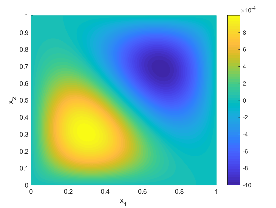 Figure 1
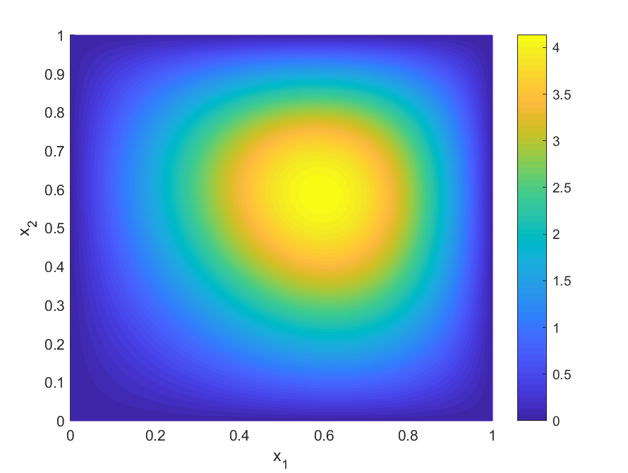 Figure 2
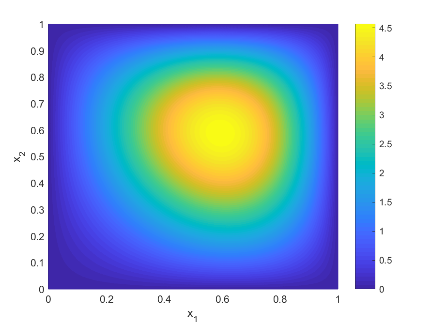 Figure 3
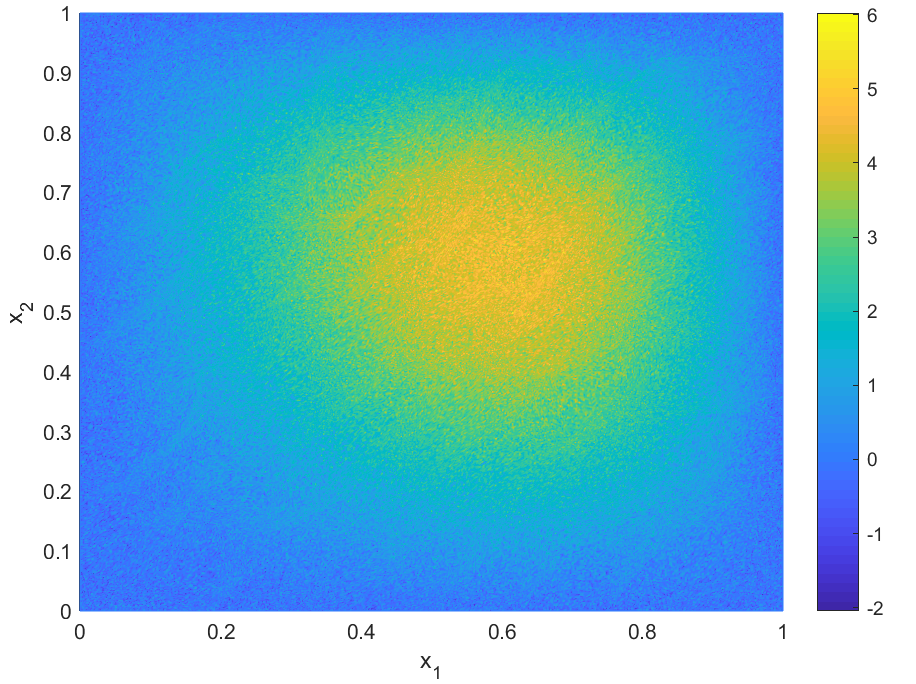 Figure 4
Peer Reviews
No public reviews on file for this paper yet. If you reviewed it on a platform where reviews are public (OpenReview, ICLR, NeurIPS, ICML), you can paste yours below so the community can read it here.
Videos
No videos yet. Explain this paper in a talk, walkthrough, or lecture? Add one.
Numerical Analysis of Sparse Initial Data Identification
for Parabolic Problems
Dmitriy Leykekhman
Department of Mathematics, University of Connecticut, Storrs, CT 06269, USA ([email protected]).
,
Boris Vexler
Chair of Optimal Control, Technical University of Munich, Department of Mathematics , Boltzmannstraße 3, 85748 Garching b. Munich, Germany ([email protected]).
and
Daniel Walter
Johann Radon Institute for Computational and Applied Mathematics, ÖAW, Altenbergerstraße 69, 4040 Linz, Austria ([email protected]). The third author gratefully acknowledges support from the International Research Training Group IGDK, funded by the German Science Foundation (DFG) and the Austrian Science Fund (FWF).
Abstract.
In this paper we consider a problem of initial data identification from the final time observation for homogeneous parabolic problems. It is well-known that such problems are exponentially ill-posed due to the strong smoothing property of parabolic equations. We are interested in a situation when the initial data we intend to recover is known to be sparse, i.e. its support has Lebesgue measure zero. We formulate the problem as an optimal control problem and incorporate the information on the sparsity of the unknown initial data into the structure of the objective functional. In particular, we are looking for the control variable in the space of regular Borel measures and use the corresponding norm as a regularization term in the objective functional. This leads to a convex but non-smooth optimization problem. For the discretization we use continuous piecewise linear finite elements in space and discontinuous Galerkin finite elements of arbitrary degree in time. For the general case we establish error estimates for the state variable. Under a certain structural assumption, we show that the control variable consists of a finite linear combination of Dirac measures. For this case we obtain error estimates for the locations of Dirac measures as well as for the corresponding coefficients. The key to the numerical analysis are the sharp smoothing type pointwise finite element error estimates for homogeneous parabolic problems, which are of independent interest. Moreover, we discuss an efficient algorithmic approach to the problem and show several numerical experiments illustrating our theoretical results.
Key words and phrases:
optimal control, sparse control, initial data identification, smoothing estimates, parabolic problems, finite elements, discontinuous Galerkin, error estimates, pointwise error estimates
1991 Mathematics Subject Classification:
65N30,65N15
1. Introduction
In this paper we consider a problem of identification of an unknown initial data for a homogenous parabolic equation
[TABLE]
from a given (measured) data of the terminal state for some . In general, this problem is known to be exponentially ill-posed, see, e.g., [17]. We are interested in the situation, where the initial data we are looking for, is known to be sparse, i.e. to have a support of Lebesgue measure zero. The strong smoothing property of the above equation makes it difficult to identify such sparse initial data. The remedy is the incorporation of the information that the unknown should be sparse in the optimal control formulation. Following the idea for measure valued formulation of sparse control problems, see, e.g., [7, 8, 9, 20, 28], we will look for the initial state in the space of regular Borel measures on the domain , which is known to be isomorphic to the dual space of continuous functions which are zero on , .
The corresponding optimal control formulation reads as follows
[TABLE]
Here and in what follows, is a convex polygonal/polyhedral domain in , , is the time interval, is the given (desired /measured) final state, and is the regularization parameter. A very similar problem is considered in [7]. There, the initial state is also searched for in the space . For given and the optimal control problem in [7] is formulated as follows:
[TABLE]
One can directly show, that problems (2) and (3) are equivalent by appropriate choices of and .
The optimal control problem (2) possesses a unique solution , see next section for details. For a numerical solution of the optimal control problem under consideration we will use discontinuous Galerkin methods dG() of order for temporal and linear (conforming) finite elements for spatial discretizations of the state equation (1) leading to the discrete optimal solution . The same type of discretization (with ) is used in [7], where weak-star convergence in for the control and strong convergence in is shown for the discretization parameters and tending to zero. However, no convergence rates with respect to or are derived in [7]. The main goal of this paper is to close this gap and obtain precise error estimates. In addition, in the case when the optimal control is in the form of linear combination of Diracs, we obtain convergence rates for the source locations and the corresponding coefficients. We illustrate the theoretical results with numerical experiments.
For the general case (i.e. without any further assumptions) we will prove the following error estimate
[TABLE]
where denotes the maximal time step, is the spatial mesh size, and is a logarithmic term, see Theorem 5 for details.
From the optimality system (see next section) we will deduce, that the support of the optimal control (optimal initial state) is contained in the set of maxima and minima of the adjoint state , see Corollary 2. Under additional assumptions (Assumption 1) on this set, which implies that the optimal control consists of finitely many Dirac measures, i.e.
[TABLE]
we will show, that the discrete optimal control has a similar structure, i.e.
[TABLE]
where each Dirac measure on the continuous level is approximated by Dirac measures on the discrete level, see Lemma 6.2 for details. In this setting we will provide (see Theorem 6.1 and Theorem 6.2) an improved error estimate for the optimal states, i.e.
[TABLE]
Moreover, we will prove an estimate for the error in position of the support points,
[TABLE]
for all and and a corresponding estimates for the coefficients. As a corollary we obtain an error estimate for the discrete optimal solutions in the norm on the topological dual of the Sobolev space . This also implies the same rate of convergence for with respect to the Kantorovich-Rubinshtein norm, [3, Section 8.3], given by
[TABLE]
for . In fact, we readily verify that this norm is equiavalent to the norm. Roughly speaking, the metric induced by the Kantorovich-Rubinshtein norm can be interpreted as an extension of the well-known Wasserstein-1 distance, [18], which is defined for probability measures, to signed measures with different mean values.
In order to obtain such convergence rates we need to revise fully discrete pointwise smoothing error estimates for a homogeneous parabolic problem
[TABLE]
with a general initial condition . This means that for the fully discrete approximation we need optimal pointwise spatial error estimates for in terms of the norm of the initial data. This problem is classical and was considered in a number of papers, we only mention the most relevant ones to our presentation. Global error estimates for smooth domains and uniform time steps were established in [16], on the other hand superconvergent results at time nodes in norm, again on smooth domains were established in [12]. One of the main contributions of our paper is the derivation of superconvergent in time and pointwise in space interior error estimates on convex polygonal/polyhedral domains. More precisely, we establish the following result
[TABLE]
where is an interior point. The precise form of the constants and the logarithmic terms are given in the statements of the Theorem 3.2 and Theorem 3.2. This result is required for our error analysis for the problem (2) and is also of independent interest.
Throughout the paper we use for the absolute value and also for the Euclidian norm of a vector in . We employ the usual notation for the Lebesgue and Sobolev spaces. We denote by the inner product in , by the duality product between and , and by the inner product in with a subinterval . With we denote the usual space
[TABLE]
The paper is organized as follows. In the next section we introduce the optimal control problem, derive first order optimality conditions and discuss structural properties of the optimal solutions. In section 3, we present a fully discrete scheme for the homogeneous parabolic equation (5) and state key smoothing error estimates, the proofs of which are postponed until sections 7 and 8. In section 4, we look separately at the time semidiscretization and the full discretization of the optimal control problem and derive some preliminary results. In section 5 we first obtain suboptimal error estimates for the general case which under additional assumptions we improve in section 6. Finally, the last two sections are devoted to the description of the algorithm and numerical illustrations of our theoretical results.
2. Optimal control problem
To introduce the precise formulation of the optimal control problem under the consideration we first discuss the solution of the state equation (1). For a given we define a (very weak) solution of (1) if the following identity holds
[TABLE]
for all , where is the weak solution of
[TABLE]
It is well known, that for , see, e.g., [15, Theorem 6.8] on general Lipschitz domains, or [4, Theorem 5.1]. Therefore, and the solution is well defined. There holds the following proposition, see [7, Lemma 2.2].
{prpstn}
For each there exists a unique solution of (1) in the above sense. Moreover, there holds for all with
[TABLE]
and with the corresponding estimates
[TABLE]
and
[TABLE]
{rmrk}
The final state has more regularity. There holds for any natural number . For example by taking , we obtain using the convexity of the domain.
The unique solvability of the state equation allows us to introduce the control-to-state mapping with . By the discussion above this operator is linear continuous and due to it maps every weakly star converging sequence to a strongly converging sequence in . Based on this operator we define the reduced cost functional by
[TABLE]
The optimal control problem (2) can then be formulated as
[TABLE]
{thrm}
The problem (7) possesses a unique solution . There holds the estimates
[TABLE]
where is the corresponding optimal state.
Proof.
The existence follows by standard arguments, cf., e.g, [9, Proposition 2.2.]. The uniqueness follows as in [7, Theorem 2.4] using density of the range of the semigroup generated by the heat equation [14], which is equivalent to the backward uniqueness property of the heat equation. The estimates follow from . ∎
The unique solution and the corresponding optimal state can be characterized by the following optimality conditions.
{thrm}
The control is the solution of (7) if and only if the triple satisfies the following conditions:
- •
state equation, in the sense of Proposition 2.
- •
adjoint equation for being the weak solution of
[TABLE]
- •
variational inequality
[TABLE]
Proof.
The proof is similar to [5, Theorem 2.1]. Note, that , which makes the duality product in the variational inequality well defined. ∎
The next lemma states additional regularity for .
{lmm}
Let be the solution of (7), be the corresponding state and the corresponding adjoint state. Let be an interior subdomain of , i.e. . Then there holds with
[TABLE]
where the constant depends on , and .
Proof.
As in Remark 2, one shows directly with
[TABLE]
cf. also (17) below. Then the elliptic interior regularity result from [13, Chapter 6.3,Theorem 2] implies
[TABLE]
where in the last estimate we used Theorem 2. ∎
From the above optimality condition we obtain the following structural properties of the optimal solution and the corresponding optimal adjoint state .
{crllr}
Let be the solution of (7), be the corresponding state and the corresponding adjoint state. Then there hold
- (a)
a bound for the adjoint state
[TABLE]
- (b)
a support condition for the positive and the negative parts in the Jordan decomposition of
[TABLE]
Moreover there is a subdomain with such that
[TABLE]
Proof.
The proof is similar to [9] or [5]. ∎
{rmrk}
The adjoint state is analytic on , see [19]. This implies by the above corollary that Lebesgue measure of is zero.
3. Discretization and smoothing type error estimates
In this section we describe the (fully discrete) finite element discretization of the (axillary) homogeneous equation (5) and present smoothing type error estimates. To discretize the problem we use continuous linear Lagrange finite elements in space and discontinuous Galerkin methods of order in time. To be more precise, we partition into subintervals of length , where . The maximal and minimal time steps are denoted by and , respectively. We impose the following conditions on the time mesh (as in [22] or [24]):
- (i)
There are constants independent on such that
[TABLE] 2. (ii)
There is a constant independent on such that for all
[TABLE] 3. (iii)
It holds .
The semidiscrete space of piecewise polynomial functions in time is defined by
[TABLE]
where is the space of polynomial functions of degree in time om with values in a Banach space . We will employ the following notation for functions with possible discontinuities at the nodes :
[TABLE]
Next we define the following bilinear form
[TABLE]
where is the duality product between and . We note, that the first sum vanishes for . The dG() semidiscrete (in time) approximation of (5) is defined as
[TABLE]
Rearranging the terms in (9), we obtain an equivalent (dual) expression for :
[TABLE]
In the sequel we require the projection operator for with for on each subinterval by
[TABLE]
In the case , is defined only by the second condition.
Next we define the fully discrete approximation scheme. For ; , let denote a quasi-uniform triangulation of with mesh size , i.e., is a partition of into cells (triangles or tetrahedrons) of diameter such that for ,
[TABLE]
hold. Let be the set of all functions in that are affine linear on each cell , i.e. is the usual space of linear conforming finite elements. We define the following three operators to be used in the sequel: discrete Laplacian defined by
[TABLE]
the projection defined by
[TABLE]
and the Ritz projection defined by
[TABLE]
To obtain the fully discrete approximation of (5) we consider the space-time finite element space
[TABLE]
We define a fully discrete cG()dG() approximation of (5) by
[TABLE]
Notice that we have the following orthogonality relations
[TABLE]
In the proofs we will use the following truncation argument. For , we let and , where is the characteristic function on the interval , for some , i.e. on for some and on the remaining time intervals. Then from (9), we have the identity
[TABLE]
Same identity holds of course for fully discrete functions . The following smoothing properties of the continuous, semidiscrete and fully discrete solutions are essential in our arguments.
3.1. Parabolic smoothing
It is well known that the solution to the homogeneous problem (5) has the following smoothing property.
[TABLE]
To get smoothing estimates in some other norms, we will frequently use the Gagliardo-Nirenberg inequality
[TABLE]
which holds for any subdomain fulfilling the cone condition (in particular for ) and for all , see [1, Theorem 3]. For it follows with the -regularity
[TABLE]
The following smoothing estimates can be obtained from (17). {lmm} Let and be the solution of (5). Then and the following estimate holds
[TABLE]
Moreover, for each interior subdomain with , the final state is (real) analytic on such and there hold
[TABLE]
Proof.
The first inequality follows right the way from (17) with by regularity. The analyticity can be found, e.g., in [19]. To prove the second inequality we first observe that
[TABLE]
Then we use Gagliardo-Nirenberg inequality (18) for and resulting in
[TABLE]
where we have used the interior regularity result [13, Chapter 6.3,Theorem 2]. To show the last inequality we use Gagliardo-Nirenberg inequality (18) for and resulting in
[TABLE]
where we again have used the interior regularity result [13, Chapter 6.3,Theorem 2] and convexity of . ∎
For the discontinuous Galerkin methods similar smoothing type estimates also hold, see Theorems 3,4,5,10 in [23] for general norms, cf. also [11, Theorem 5.1] for the case of the norm. {lmm}[Smoothing estimate] Let and be the semidiscrete and fully discrete solutions of (10) and (14), respectively. Then, there exists a constant independent of and such that
[TABLE]
for and any . For the jump term is understood as and .
In addition the stability with respect to the norm is valid for the semidiscrete and fully discrete approximations of the heat equation. For the proof we refer to [23, Lemma 5], see also [27]. {lmm} Let and be the semidiscrete and fully discrete solutions of (10) and (14), respectively. Then, there exists a constant independent of and such that
[TABLE]
holds for any .
From Lemma 3.1 we immediately obtain the following corollary. Note, that the corresponding estimate is not true on the continuous level, which explains the presence of the logarithmic term. {crllr} Under the assumptions of Lemma 3.1, for any we have
[TABLE]
and
[TABLE]
Proof.
We only provide the proof for the semidiscrete case, the fully discrete case is identical. Using the above smoothing result from Lemma 3.1, we have
[TABLE]
where in the last step we used that
[TABLE]
∎
For sufficiently many time steps, applying Lemma 3.1 iteratively, we immediately obtain the following result. {lmm} Let and be the semidiscrete and fully discrete solutions of (10) and (14), respectively. For any , any , and any there hold
[TABLE]
and
[TABLE]
provided .
The next lemma is the semidiscrete analog of Lemma 3.1. {lmm} Let and be the semidiscrete solution of (10). Let be an interior subdomain, i.e. . Then and the followings estimates hold
[TABLE]
Proof.
The proof is similar to the proof of Lemma 3.1 and uses Lemma 3.1. ∎
Using the discrete version of the Gagliardo-Nirenberg inequality
[TABLE]
which for example was established for smooth domains in [16, Lemma 3.3], but the proof is valid for convex domains as well, we immediately obtain the following smoothing result. {crllr} Under the assumption of Lemma 3.1 for all , we have
[TABLE]
3.2. Smoothing pointwise error estimates
One of the main tools in obtaining error estimates for the optimal control problem under consideration are the pointwise smoothing error estimates that have an independent interest. The next theorems show that for the error at a point we can obtain nearly optimal convergence rates in space and superconvergent rates in time. For elliptic problems such interior pointwise elliptic results are known from [30, 31]. For homogeneous parabolic problems with smoothing such results are new.
The first theorem provides an error estimate for the semidiscrete error .
{thrm}
Let , let and satisfy (5) and (10). Then there holds
[TABLE]
with .
Note, that we obtain here a superconvergent estimate of order for the discretization with polynomials of order . The proof of this theorem is given in Section 7.
{rmrk}
In the sequel we will apply this and the following theorems for both, a heat equation formulated forward in time (5) and for a heat equation formulated backward in time, i.e.
[TABLE]
for some . Its semidiscrete approximation solves
[TABLE]
For this case the statement of the above theorem reads
[TABLE]
Correspondingly we will apply also Theorem 3.2 and Theorem 3.2 for this setting.
A corresponding result is true also for the norm of the gradient.
{thrm}
Let , let and satisfy (5) and (10). Let moreover with be an interior subdomain. Then there holds
[TABLE]
with .
The proof of this theorem is given in Section 7. {rmrk} The result of Theorem 3.2 is valid also on the whole domain instead of with a slightly different constant .
For the spatial error we can not expect an estimate with respect to the global norm. However for a given point we obtain the following result.
{thrm}
Let , let and satisfy (10) and (14), respectively and let such that with . Then there holds
[TABLE]
where and is a constant, which explicit dependence on and can be tracked from the proof.
The proof of this theorem is given in Section 8. Combining both theorems we immediately obtain an estimate for . {crllr} Let , let and satisfy (5) and (14), respectively and let such that with . Then there holds
[TABLE]
where .
4. Discretization of optimal control problem
In this section we describe the temporal and spatial discretizations of the optimal control problem (2).
4.1. Temporal semidiscretization
To introduce the associated semidiscrete state for a given control we consider slightly modified semidiscrete spaces defined by
[TABLE]
and
[TABLE]
with some and with . For this setting we have for all due to the embedding . The bilinear form from (9) can be extended to . This allows us to define the semidiscrete state by
[TABLE]
The corresponding semidiscrete control-to-state mappings is given by and the semidiscrete reduced cost functional by
[TABLE]
With this reduced cost functional we formulate the semidiscrete optimal control problems without discretization of the control space as follows:
[TABLE]
As on the continuous level we obtain the existence of a solution to (23). {thrm} The problem 23 possesses at least one solution with corresponding state . There hold the estimates
[TABLE]
Proof.
The existence and the estimates follow by standard arguments, as on the continuous level. ∎
The question of uniqueness of is more involved and is discussed after the statement of the optimality system.
{thrm}
The control is a solution of (23) if and only if the triple fulfills the following conditions:
- •
semidiscrete state equation, in the sense of (22).
- •
semidiscrete adjoint equation for being the solution of
[TABLE]
- •
variational inequality
[TABLE]
Proof.
The proof is the same as for the continuous problem. ∎
{crllr}
Let be a solution of (23), be the corresponding state, and the corresponding adjoint state. Then there hold
- (a)
a bound for the adjoint state
[TABLE]
- (b)
a support condition for the positive and the negative parts in the Jordan decomposition of
[TABLE]
Moreover there is a subdomain with such that
Proof.
The proof is the same as for the continuous problem. ∎
The uniqueness of the solution on the continuous level follows (cf. [7, Theorem 2.4]) by the fact that for the solution of the heat equation (5) we have that implies . This is also true for the discretization but is in general wrong for the dG() semidiscretization with . However, the following technical lemma allows us to prove uniqueness of the semidiscrete control .
{lmm}
Let and be the corresponding semidiscrete state defined by (22). Let . Then the holds:
- (1)
For we have . 2. (2)
Let . If there exists an open set such that , then .
Proof.
It is well known, cf., e.g., [12], that dG() discretization of a homogeneous problem coincides with the corresponding subdiagonal Padé approximation scheme. Therefore, there is a rational function with polynomials , and for , such that
[TABLE]
By the assumption of the lemma we have .
- (1)
For we have and therefore
[TABLE]
which implies . Similarly, we obtain for all and consequently . 2. (2)
For we argue differently. We consider the eigenvalues of and the corresponding system of eigenfunctions with . The initial condition can be expanded as
[TABLE]
and the convergence to be understood in . We define the polynomials
[TABLE]
With this notation we have
[TABLE]
and consequently . This results is
[TABLE]
and therefore
[TABLE]
Assume now that . Since has no more than positive zeros, there are only finitely many with . For this reason we have that the expansion (24) is a finite sum and therefore since for every by convexity of . We have with some
[TABLE]
From and we obtain that also vanishes on for every . Therefore, we have
[TABLE]
and dividing by we have
[TABLE]
For all summands with converge to zero resulting in
[TABLE]
This is an eigenfunction of , which provides a contradiction, since a nontrivial eigenfunction can not vanish on an open set by the unique continuation principle, see, e.g., [21, p. 64]. This completes the proof.
∎
{thrm}
The solution of (23) is unique.
Proof.
We first observe the uniqueness of by the strict convexity of the tracking term in . It remains to show, that this implies the uniqueness of . Assume there are two optimal controls and consider the difference . Let , i.e. . Then there holds . In the case we immediately obtain by the first statement of Lemma 4.1. For we obtain from Corollary 4.1, that with and therefore . This implies the existence of an open set with . Then we obtain from the second statement of Lemma 4.1. ∎
4.2. Space-time discretization
For a given control we also introduce the associated fully discrete state by
[TABLE]
the fully discrete control-to-state mappings by , and the fully discrete reduced cost functional by
[TABLE]
Based on this definition we formulate the corresponding optimal control problem, where we first look for the control variable in the whole space . This leads to the following formulation.
[TABLE]
One can not expect, that this problem has a unique solution. For however, where is a unique solution in the properly defined discrete subspace of , see the discussion below. To introduce the space , let be the set of all interior nodes of the mesh . For let denote the Dirac measure concentrated in and be the nodal basis function associated to the node . Then we define the space as
[TABLE]
and introduce a projection operator (cf., e.g., [5]) by
[TABLE]
The definition implies that
[TABLE]
where is the nodal interpolation operator. The following two properties of can be directly checked. {lmm} There holds
- (a)
for all .
- (b)
The fully discrete solutions of the state equation associated with and with are the same, i.e.
[TABLE]
Proof.
The proof of (a) follows from [6, Thm. 3.1] and the proof of (b) uses the definition (25) of and (27). ∎
The next theorem provides the existence of a solution to (26). {thrm} There exists a solution of (26). For each solution the projection is also a solution of (26). For the solution is unique. For any solution and the corresponding state the following estimates hold
[TABLE]
Proof.
The existence and the estimates follow as on the continuous level. The fact that is also a solution of (26) follows directly from Lemma 27. The uniqueness in the case of follows from the fully discrete analog of the first statement of Lemma 4.1, cf. also the proof of [7, Theorem 4.8]. ∎
{rmrk}
For it seems that problem (26) may in general have multiple solutions in . The argument we used to prove uniqueness of the semidiscrete solution is based on the second statement of Lemma 4.1, which does not extend to the fully discrete setting.
In the next theorem we state the optimality system on the fully discrete level. {thrm} The control is a solution of (26) in if and only if the triple fulfills the following conditions:
- •
fully discrete state equation, in the sense (25).
- •
fully discrete adjoint equation for being the solution of
[TABLE]
- •
variational inequality
[TABLE]
Proof.
The proof is the same as for the continuous problem. ∎
{rmrk}
Please note, that the variational inequality in the above theorem holds for all variations and not only for those from . This is due to the fact that the solution solves the problem (26), where the control is not discretized, see Theorem 4.2.
{crllr}
Let be a solution of (26), be the corresponding state and the corresponding adjoint state. Then there hold
- (a)
a bound for the adjoint state
[TABLE]
- (b)
a support condition for the positive and the negative parts in the Jordan decomposition of
[TABLE]
Moreover there is a subdomain independent on and with such that
Proof.
The proof is the same as for the continuous problem. ∎
5. General error estimates for the optimal control problem
In this section we prove an error estimate for the error between the optimal state on the continuous and on the discrete level, which does not require any further assumptions on the structure of the solution.
As the first step we provide an estimate for the error in the state at terminal time for a given control .
{lmm}
Let be a given control with and . Let be the solution of the state equation (1), be the semidiscrete approximation (22) and the fully discrete approximation (25). Then there hold
[TABLE]
and
[TABLE]
where .
Proof.
To prove the first estimate we consider the solution of the dual problem
[TABLE]
and its semidiscrete approximation solving
[TABLE]
There holds
[TABLE]
where in the last step we used Theorem 3.2 for the error in the norm, see also Remark 3.2.
For the proof of the spatial estimate we consider the dual solution solving
[TABLE]
and solving
[TABLE]
Then we get
[TABLE]
where we used the fact that and Theorem 3.2 in the last step.
∎
{rmrk}
Please note that the assumption with in the above theorem is required only for the spatial estimate.
Based on this theorem we can directly obtain estimates for optimal values of the cost functional.
{thrm}
Let be the optimal solution of (7) with the corresponding optimal state . Let be the optimal solution of the semidiscrete problem (23) with the corresponding state and let be a solution of the fully discrete problem (26) with the corresponding state . Then there hold:
[TABLE]
and
[TABLE]
where and depends on and .
Proof.
By the optimality of for (7) we have
[TABLE]
Similarly by the optimality of for (7) we have
[TABLE]
and therefore
[TABLE]
For both and we estimate
[TABLE]
Then using the first estimate from Lemma 5, the estimates
[TABLE]
as wells as estimates for and from Theorem 2 and Theorem 4.1 we complete the proof for the temporal error. The spatial error is estimated similarly by using the second estimate from Lemma 5. ∎
The next theorem is the main result of this section, which provides an estimate for the error between the optimal states.
{thrm}
Let be the optimal solution of (7) with the corresponding optimal state . Let be the optimal solution of the semidiscrete problem (23) with the corresponding state and let be a solution of the fully discrete problem (26) with the corresponding state . Then there hold:
[TABLE]
and
[TABLE]
where and depends on , and .
Proof.
To prove the first estimate we use the variational inequality from Theorem 2 with
[TABLE]
and the corresponding variational inequality from Theorem 4.1 with
[TABLE]
Adding these two inequalities results in
[TABLE]
To proceed we introduce as the solution of (22) for and fulfilling
[TABLE]
Using the semidiscrete state and adjoint equations we obtain
[TABLE]
This results in
[TABLE]
By the Cauchy-Schwarz inequality in the last term and absorbing in the left-hand side we obtain
[TABLE]
Using the estimates for and from Theorem 2 and Theorem 4.1 we get
[TABLE]
For the term we can directly apply Theorem 3.2 resulting in
[TABLE]
The term is estimated by the first estimate in Lemma 5 leading to
[TABLE]
Putting these estimates together we obtain
[TABLE]
which is the the first desired estimate. The estimate for is obtained similarly using Theorem 3.2 and the second estimate from Lemma 5. ∎
For the error in the control we can in general only expect a weak star convergence, see the following lemma. {lmm} Let be the optimal solution of (7), be the optimal solution of the semidiscrete problem (23), and be a solution of the fully discrete problem (26). Then there holds
[TABLE]
and for fixed
[TABLE]
Proof.
The proof is similar to the proof of [7, Theorem 4.10]. ∎
Under an additional assumption stronger results are discussed in the next section.
6. Improved error estimates for the optimal state and control
In the previous section we provided error estimates for the error in the cost functional and for the optimal states at the terminal time. In general we can not expect an error estimate for the control, , with respect to the norm in , since only weak star convergence of the controls can be expected, cf. the corresponding discussion in [7]. However, if the optimal control consists of finitely many Diracs, error rates for the positions and the coefficients of these Diracs can be shown. To prove such error estimates and to improve the estimate for the state from Theorem 5 we make the following assumption.
Assumption 1**.**
Let be the solution of the problem of (7) with the corresponding optimal state and adjoint state . We assume that
[TABLE]
with and for are pairwise disjoint points. Moreover, there holds
[TABLE]
and
[TABLE]
where denotes the Hessian matrix of with respect to the spatial variable.
{rmrk}
- •
From Corollary 2 (b) we have that
[TABLE]
Here, we assume equality of these two sets and the finite cardinality of them.
- •
Due to the fact by Corollary 2 (a), the points with are the minimizers and the points with are the maximizers of . Therefore, we have and the corresponding Hessian matrices are positive semidefinite in the former and negative semidefinite in the later case. In addition we assume positive and negative definiteness respectively. This assumption corresponds to sufficient second order optimality conditions for minimizers and maximizers of .
- •
Similar assumptions can be found in the literature, see [25, 32] in the context of semi-infinite programming and the notion of non-degeneracy in super-resolution [10].
Under the above assumption the optimal control consists of finitely many Diracs and has the form
[TABLE]
with , where for with and for with .
6.1. Error estimates for the temporal error
We first prove that under Assumption 1 the structure of the semidiscrete control is similar to that of (30). To this end we first show that Hessian matrix of the discrete adjoint state has the same definiteness properties as of the continuous adjoint state in the neighborhoods of the points . {lmm} Let Assumption 1 be fulfilled. Let be the optimal solution of the semidiscrete problem (23) with the corresponding state and the adjoint state . Then there exist , , and such that
[TABLE]
for all and all for with , where denotes the smallest eigenvalue of the corresponding matrix. Similarly,
[TABLE]
for all and all for with .
Proof.
We consider with . The Hessian matrix is positive definite by Assumption 1. Moreover by Lemma 2. Therefore, there exists a neighborhood such that is uniformly positive definite for . It remains to prove that
[TABLE]
There holds
[TABLE]
by the embedding , the interior regularity result [13, Chapter 6.3,Theorem 2] and convexity of . To proceed we insert defined by (28) leading to
[TABLE]
The first term is directly estimated by Lemma 7 (below) with resulting in
[TABLE]
and for the second term we have by the smoothing estimate Lemma 3.1
[TABLE]
where in the last step we used the first estimate from Theorem 5. This completes the proof. ∎
{lmm}
Let Assumption 1 be fulfilled. Let be the optimal solution of the semidiscrete problem (23) with the corresponding state and the adjoint state . Then there is an and such that the neighborhoods are pairwise disjoint and for each and there is a unique such that
[TABLE]
and
[TABLE]
Moreover there are no further points with and the semidiscrete control has the structure
[TABLE]
with , where for with and for with .
Proof.
First we choose such that the statement of Lemma 6.1 are fulfilled for all and the balls are pairwise disjoint. Let be fixed with . The case of is discussed in the same fashion. From Lemma 5 we have in . We choose a smooth cut-off function with for all and with . From the weak star convergence we obtain
[TABLE]
Therefore, there exists such that for all , which proves that is not empty. The support condition for from Corollary 4.1 implies the existence of at least one with . By Lemma 6.1 is strictly convex on . This implies the uniqueness of the minimizer in . In order to show that there are no further points with in the complement of the union of all , it is sufficient to show that for . We have as in the proof of the previous lemma
[TABLE]
where is defined by (28). For the first term we obtain by Theorem 3.2
[TABLE]
and for the second one
[TABLE]
where in the last step we used the first estimate from Theorem 5. This completes the proof. ∎
The main result of this section provides optimal order estimates for the error in the position , the coefficients and improves the first estimate from Theorem 5 for the state error .
{thrm}
Let be the solution of the problem of (7) with the corresponding optimal state and the adjoint state and let Assumption 1 be fulfilled. Let moreover be the optimal solution of the semidiscrete problem (23) with the corresponding state and the adjoint state . Then there exists such that for there hold
- (a)
[TABLE]
- (b)
[TABLE]
- (c)
[TABLE]
- (d)
[TABLE]
where depends on , and .
{rmrk} From the equivalence relation in (LABEL:eqofwinfkr) we directly infer
[TABLE]
from statement (d) above.
To prepare the proof of Theorem 6.1 we first estimate the error in the position and in the coefficients in terms of the state error .
{lmm}
Let Assumption 1 be fulfilled. Then there exists such that for there holds
[TABLE]
for all , where depends on and .
Proof.
For a fixed we assume without restriction that (the case can be treated similarly). Then we have that by Lemma 6.1. The point is a minimizer of and the point is a minimizer of . Therefore, there holds
[TABLE]
Due to the fact that is uniformly positive definite on and we have
[TABLE]
and therefore
[TABLE]
where is the solution of the intermediate discrete adjoint equation (28) and is an interior subdomain with
[TABLE]
By Theorem 3.2 we have
[TABLE]
and by the smoothing property from Lemma 3.1
[TABLE]
This completes the proof. ∎
To proceed we introduce the operators by
[TABLE]
where and are the continuous and the semidiscrete solution operators defined above. Moreover we restrict the codomains of these operators to the corresponding image sets and call the resulting operator , and with
[TABLE]
and
[TABLE]
In the next lemma we estimate the errors between these operators. {lmm} Let Assumption 1 be fulfilled. There hold
[TABLE]
and
[TABLE]
Proof.
For given we consider defined by
[TABLE]
as well as the corresponding states , in the sense of Proposition 2 and in the sense of (22). The second statement is then directly given by Lemma 5, since
[TABLE]
To prove the first statement we consider a dual problem for solving
[TABLE]
and obtain
[TABLE]
where in the last step we used smoothing estimate from Lemma 3.1 for . This completes the proof. ∎
{lmm}
Let Assumption 1 be fulfilled. The operators , are bijective and there is a constant such that
[TABLE]
hold for all . Moreover, there is such that is bijective and the estimate
[TABLE]
holds for all and all .
Proof.
All three operators , and are surjective by definition. We first argue the injectivity of . Let for some . This means that for the solution of the heat equation with the initial condition given as the corresponding linear combination of Diracs, i.e. , we have . By a similar argument as in proof of uniqueness of the optimal control , cf. [7, Theorem 2.4], we obtain
[TABLE]
This results in by the fact that the points are pairwise disjoint. This provides the existence of an inverse mapping and the estimate
[TABLE]
holds. For the operator we can argue similarly. It remains to show that is bijective and is bounded independently of . Let be arbitrary. There holds by (32) and Lemma 6.1
[TABLE]
where in the last step we used Lemma 6.1 and Theorem 5. Choosing small enough we obtain
[TABLE]
which completes the proof. ∎
{lmm}
Let Assumption 1 be fulfilled. Then there exists such that for there holds
[TABLE]
where depends on and .
Proof.
There holds by Lemma 6.1
[TABLE]
By the definition we have and . Using Lemma 6.1 and Lemma 6.1 we obtain
[TABLE]
The fact that
[TABLE]
completes the proof. ∎
Previous lemmas allow us to obtain the corresponding estimate for a negative norm of in terms of .
{lmm}
Let Assumption 1 be fulfilled. Let be the solution of (7) and be the solution of the semidiscrete problem (23). Then there holds
[TABLE]
Proof.
Let with . We have to estimate
[TABLE]
Using Lemma 6.1 and Lemma 6.1 we obtain
[TABLE]
which completes the proof. ∎
We proceed with the proof of Theorem 6.1.
Proof.
We start with the estimate (29) from the proof of Theorem 5, i.e.
[TABLE]
where and is the solution of (28). The second term can be estimated as in the proof of Theorem 5 by the first estimate in Lemma 5 leading to
[TABLE]
It remains to estimate the duality product from (33). We have by Lemma 6.1
[TABLE]
where we have used the fact that . Using Theorem 3.2 and Theorem 3.2 we have
[TABLE]
Putting all terms in (33) together we get
[TABLE]
Absorbing in the left-hand side we obtain the estimate (a) in Theorem 6.1. The estimates (b), (c), and (d) are obtained from (a) using Lemma 6.1, Lemma 6.1 as well as Lemma 6.1. ∎
6.2. Error estimates for the spatial error
For the semidiscretization we have shown (see Lemma 6.1) that the number of support points of the semidiscrete control is the same as on the continuous level in Assumption 1. For the fully discrete control the situation is different. We will show (see next lemma) that in the neighborhood of each support point of there is at least one support point of , but there could be more than one such point. This phenomena is also observed in our numerical experiments.
{lmm}
Let Assumption 1 be fulfilled. Let be the optimal solution of the semidiscrete problem (23) with the corresponding state and the adjoint state . Let be an optimal solution of the fully discrete problem (26) with the corresponding state and the adjoint state . Then there is such that for any fixed the following holds. There is an and such that the neighborhoods are pairwise disjoint and for each and there is at least one such that
[TABLE]
and
[TABLE]
Moreover there are no points with .
Proof.
The proof is similar to the proof of Lemma 6.1. ∎
Under the conditions of Lemma 6.2 a fully discrete control consists of groups of Dirac functionals for each single Dirac on the semidiscrete level. This means, that is given as
[TABLE]
where describes the cardinality of . The cardinality of is then . In order to compare the vector of coefficients with the vector on the semidiscrete level, we define by
[TABLE]
The next theorem is the main result of this section. {thrm} Under the conditions of Lemma 6.2 there holds
- (a)
[TABLE]
- (b)
[TABLE]
for all and .
- (c)
[TABLE]
- (d)
[TABLE]
where .
{rmrk} As in Remark 6.1, we directly conclude the a priori estimate
[TABLE]
from statement (d) in Theorem 6.2.
To prove Theorem 6.2 we start with the lemma providing a sub-optimal estimate for the distance between the support points of and .
{lmm}
Under the conditions of Lemma 6.2 there is a constant such that for each with there holds
[TABLE]
where .
Proof.
We consider the Taylor expansion with an appropriate
[TABLE]
where we used that by the previous lemma and by the optimality of for , see Corollary 4.1 and Lemma 6.1. Using uniform definiteness of , see Lemma 6.1, we obtain
[TABLE]
where is an interior subdomain with
[TABLE]
see Corollary 4.1 and Corollary 4.2. To proceed we introduce an intermediate discrete adjoint state fulfilling
[TABLE]
We obtain
[TABLE]
The first term is estimated by Theorem 3.2 leading to
[TABLE]
and the second term by the smoothing property from Corollary 3.1 and by the second estimate from Theorem 5
[TABLE]
This completes the proof. ∎
For the proof of Theorem 6.2 we introduce a further intermediate adjoint state defined by
[TABLE]
{lmm}
Let the conditions of Lemma 6.2 be fulfilled and let be defined by (35). Then for each with there is a minimizer of and for each with there is a maximizer of . Moreover there holds
[TABLE]
Proof.
Without restriction we assume that and from Lemma 6.2 are chosen such that the statement of Lemma 6.1 holds. We fix with and introduce two functions by
[TABLE]
There holds by the optimality of for that and by Lemma 6.1 that is positive definite. Moreover we have
[TABLE]
and
[TABLE]
by the smoothing property from Lemma 3.1 and the estimate from Theorem 5. In addition is Lipschitz continuous on with the Lipschitz constant
[TABLE]
where we have used interior estimate as in the proof of Lemma 3.1. In this setting we can apply [29, Theorem 3.1] to get the existence of (for ) with and a positive definite , such that
[TABLE]
This completes the proof. ∎
In the next lemma we improve the estimate from Lemma 6.2. {lmm} Let the conditions of Lemma 6.2 be fulfilled. Then there holds for all and all
[TABLE]
Proof.
We fix an with and an . For defined in (35) we observe
[TABLE]
by Theorem 3.2. Due to Corollary 4.1 we have for all and therefore
[TABLE]
Using the Taylor expansion and the fact that we get with some
[TABLE]
where we have used that is uniformly positive definite on by the positive definiteness of and (36). This results in
[TABLE]
This completes the proof. ∎
We proceed with the proof of Theorem 6.2.
Proof.
The first statement is already shown in Theorem 5. The second statement follows directly from Lemma 6.2 and Lemma 6.2 by the triangle inequality. It remains to prove statements (c) and (d). To this end we will use the operator introduced in (31). Similarly we introduce the operator by
[TABLE]
Without restriction we assume that from Lemma 6.2 is chosen such that the statement of Lemma 6.1 holds. Then we obtain similarly to the proof of Lemma 6.1 using
[TABLE]
The first term is estimated by Theorem 5
[TABLE]
the last term is estimated by Lemma 5 leading to
[TABLE]
To estimate the second term in (37) we observe that
[TABLE]
For a given we get for the inner difference using
[TABLE]
Then by a duality argument as in the proof of Lemma 6.1 we obtain
[TABLE]
resulting in
[TABLE]
by the statement (b). Inserting this into (37) completes the proof of the statement (c). To prove statement (d) let with be given. We estimate
[TABLE]
Using statements and from Theorem 6.2 as well as the boundedness of we obtain
[TABLE]
which completes the proof. ∎
7. Proof of smoothing error estimates in time
In this section we prove Theorem 3.2 and Theorem 3.2. First we establish the following result.
{lmm}
Let , let and satisfy (5) and (10). Then for , there exists a constant independent of and such that
[TABLE]
Proof.
For any , let be the solution to the following backward problem
[TABLE]
and be its dG() approximation, i.e.
[TABLE]
Using the orthogonality conditions (15a) and the dual representation of the bilinear form (11)
[TABLE]
where is the projection defined in (12). Note, the jump terms vanish by the definition of . We set and . Using the approximation and the standard energy estimate we have
[TABLE]
Using the properties of the bilinear form (9), we have
[TABLE]
Canceling and using (38) we obtain
[TABLE]
Combining (38) and (39) we also have
[TABLE]
Next we estimate . By the triangle inequality, inverse inequality and (38), (39), and (40) we obtain
[TABLE]
This allows to estimate as follows
[TABLE]
Similarly, using approximation and (40) we obtain for
[TABLE]
Combining the estimates for and and canceling , we obtain the lemma. ∎
Now we show the next result.
{lmm}
Let , let and satisfy (5) and (10). Then for provided and , there exists a constant independent of such that
[TABLE]
where .
Proof.
For any , let and be the solutions to the continuous and to the semidiscrete dual problems with , i.e. solving
[TABLE]
and satisfying
[TABLE]
We choose such that and define as well as , i.e. and are zero on and and on the remaining time intervals. Then we test (42) with and choose in (43). Using (16), we have
[TABLE]
Note, that and by construction. Using the Cauchy-Schwarz inequality, Lemma 7 with and and the smoothing estimate (17)
[TABLE]
Similarly, using the Cauchy-Schwarz inequality, Lemma 7 with and and the semidiscrete smoothing estimate in Lemma 3.1
[TABLE]
Combining the estimates for and and canceling on both sides, we obtain the lemma. ∎
7.1. Proof of Theorem 3.2
We use the Gagliardo-Nirenberg inequality (19) and obtain
[TABLE]
Application of Lemma 7 with and yields the result.
7.2. Proof of Theorem 3.2
We use Gagliardo-Nirenberg inequality (18) with as in the proof of Lemma 3.1 and obtain
[TABLE]
Application of Lemma 7 with , , and yields the result.
8. Proof of smoothing error estimates in space
In this section we prove Theorem 3.2. Before we provide the proof we show the following results. {lmm} Let and be the semidiscrete and fully discrete solutions of (10) and (14), respectively. Then there exists a constant independent of , , and such that
[TABLE]
Proof.
Let be the solution to a dual problem with , i.e.
[TABLE]
Then taking by the Galerkin orthogonality, the stability of the projection, the standard elliptic error estimates, Lemma 3.1 and Corollary 3.1, we obtain
[TABLE]
Canceling, we obtain the result. ∎
In order to establish optimal pointwise error estimates for , we first show the corresponding estimate with respect to the norm and then for in the norm likewise. {lmm} Let and be the semidiscrete and fully discrete solutions of (10) and (14), respectively. There exists a constant independent of , , and such that
[TABLE]
Proof.
Let be the solution to a dual problem with , i.e. satisfies
[TABLE]
We abbriviate and set to be zero on for such that and on the remaining time intervals. Similarly we define . Then by (16) and using the Galerkin orthogonality, we have
[TABLE]
Using (11) and the property of the Ritz projection, we have
[TABLE]
By the Lemma 3.1 and Lemma 3.1 we obtain
[TABLE]
By the approximation properties of the Ritz projection, regularity, and using the fact that we have
[TABLE]
Canceling, be obtain the result for .
To estimate we add and subtract . Thus we obtain
[TABLE]
Similarly to the above, using Lemma 3.1 and Lemma 3.1 we obtain
[TABLE]
To estimate we use Lemma 8 with and the fact the constant there does not depend on together with Lemma 3.1. Hence,
[TABLE]
Canceling, we obtain the lemma. ∎
Next we establish the following smoothing result in norm with discrete Laplacian. {lmm} Let and be the semidiscrete and fully discrete solutions of (10) and (14), respectively. There exists a constant independent of , , and such that
[TABLE]
Proof.
Let be the solution to a dual problem with , i.e. satisfies
[TABLE]
As in the proof of the previous lemma we abbriviate and set to be zero on for some to be specified later and on the remaining time intervals. Similarly we define . Then setting and using the Galerkin orthogonality and (16), we have
[TABLE]
Choosing such that , using the definition of the bilinear form , the discrete maximal parabolic regularity from Corollary 3.1 and Lemma 3.1 we obtain
[TABLE]
Canceling we obtain the desired estimate for .
To estimate we proceed as in the proof of the previous lemma,
[TABLE]
Similarly to the above,
[TABLE]
To estimate , we proceed as in the proof of the previous lemma, and using Lemma 8, we have
[TABLE]
Canceling we obtain the lemma. ∎
As a consequence of the two lemmas above and the discrete Gagliardo-Nirenberg inequality (21) we immediately obtain the following result. {lmm} Let and be the semidiscrete and fully discrete solutions of (10) and (14), respectively. Then, there exists a constant independent of and such that
[TABLE]
{rmrk}
The result in Lemma 8 is rather interesting and of independent interest. It shows that the error between the semidiscrete solution and its Ritz projection for piecewise linear elements is of optimal second order even if the exact solution at a final time is not in as for example in the case if the domain has strong corner singularities. This in particular shows a well-known fact that the presence of corner singularities is essentially an elliptic problem.
Similar to the results in [33], it also can be used to show a superconvergent result for the gradient. Thus for using the discrete Sobolev inequality
[TABLE]
we also have the following superconvergent estimate
[TABLE]
8.1. Proof of Theorem 3.2
Adding and subtracting , we have
[TABLE]
From Lemma 8 we have
[TABLE]
Using the pointwise interior elliptic results from [30] we have
[TABLE]
where we used the embedding , the interior regularity result [13, Chapter 6.3,Theorem 2] and convexity of .
9. Algorithmic treatment
This section is devoted to the algorithmic solution of the sparse initial data identification problem under consideration. Let us first note that by Theorem 4.2 we can look for a minimizer in the space consisting of linear combinations of Diracs concentrated in the interior nodes of the mesh, i.e.
[TABLE]
where is a vector of optimal coefficients. Thus, the fully discrete problem (26) can be equvalently reformulated as a finite dimensional problem (of dimension ) in the coefficients with an regularization term leading to
[TABLE]
This problem can be solved by a variety of efficient solution algorithms, e.g., semi-smooth Newton methods, [26], or FISTA, [2]. However, a direct application of finite dimensional optimization algorithms to this problem may lead to mesh-dependent methods, whose convergence behavior critically depends on the fineness of the discretization. In contrast, we employ an optimization algorithm, which can be described on the continuous level, as a solution algorithm for the problem (7). This algorithm can be then directly adapted to the discretized problem (26). Since the convergence properties of the presented algorithm can be analyzed on the continuous level, see [34], one expects mesh independent behavior for the discretized problem, which is also confirmed by our numerical results.
We propose a version of the Primal-Dual-Active-Point (PDAP) method from [34] which iteratively generates a sequence of finite linear combinations of Dirac delta functions. The algorithm on the continuous level is briefly described and its convergence properties are summarized below. Given an ordered set of finitely many points define the parametrization
[TABLE]
as well as the finite dimensional subproblem
[TABLE]
We initialize the proposed algorithm with a sparse initial iterate , . In the -th iteration, a new support point is determined based on the violation of the condition (a) in Corollary 2 by the current adjoint state . Subsequently, the new iterate is found as where is a solution to (47) for . Thus, the method alternates between updating the active set by adding to the support of the current iterate and computing a minimizer of over . The procedure is summarized in Algorithm 1.
Note that the support of is pruned after each iteration i.e. Dirac delta functions with zero coefficients are removed from the iterate. Additionally, we observe that Algorithm 1 is monotonous, i.e. , and thus also for all . To monitor the convergence of the algorithm we consider the primal-dual-gap functional which is defined as
[TABLE]
and . This is justified by the following lemma, see [34, Lemma 6.12 and Lemma 6.41]. {lmm} There holds for all with equality if and only if is the optimal solution of (7). Furthermore we have
[TABLE]
Let denote the sequence generated by Algorithm 1. Then we obtain
[TABLE]
for .
We point out that, due to (48), the primal-dual-gap can be cheaply computed as a byproduct of step .
The following theorem, see [34, Theorem 6.43], provides two convergence results. For the general case we obtain sub-linear convergence of the the cost functional. Under Assumption 1, we obtain linear convergence for the functional, positions of the Diracs and for the corresponding coefficients. {thrm} Let the sequence be generated by Algorithm 1 starting from . Then we have
[TABLE]
for all and a constant . If Assumption 1 holds, then and there exist , with
[TABLE]
as well as
[TABLE]
for all large enough.
We emphasize that the adaption of Algorithm 1 to the discrete problem (26) is straightforward. In detail, we replace the control-to-state operator by its fully discrete counterpart and compute . Moreover, in view of Theorem 4.2, the search for the maximizer in step can be restricted to the set of interior nodes . The new coefficient vector is then found as solution to the finite-dimensional subproblem
[TABLE]
Note, that the support of usually consists of only few points, i.e. the dimension of the subproblem (49) is small the this subproblem can be solved efficiently by existing finite dimensional algorithms. In our numerical realization we use the semi-smooth Newton method for the solution of (49).
10. Numerical examples
The final section is devoted to the presentation of numerical experiments which serve to underline the practical applicability of the proposed sparse control approach as well as to verify the derived theoretical results. Throughout the section, the spatial domain is given by the unit square and the final time is set to . All arising discrete optimal control problems are solved by an adaptation of the PDAP method, Algorithm 1, as described at the end of the previous section.
10.1. Identification of point sources
First, we aim to identify a sparse source term from noisy observations of . The time interval is uniformly partitioned into subintervals, the spatial domain is divided into triangles, see the description in Section 3. We emphasize that the support points and , respectively, correspond to nodes of the triangulation. For the discretization of the state equation a cG()dG([math]) (i.e ) approximation is considered. The observations are given by where is a given noise term. We plot alongside in Figure 1.
To reconstruct from the given final time observation we propose to solve with . For the described example we empirically determine as a suitable regularization parameter. Applying the Primal-Dual-Active-Point method to yields a reconstruction with . By a closer inspection, two of its support points are located in adjacent nodes of the triangulation. A possible explanation for this clustering of support points is provided by Theorem 4.2. More in detail, a spike appearing in a discrete optimal solution at an off-grid location will appear as several nodal Dirac delta functions in the projected solution . For a better visualization of the results we replace the Dirac delta functions associated to the clustering support points by a single one of the same combined mass located at the center of gravity of the original positions. The post-processed measure is depicted in Figure 2 together with .
As predicted by Corollary 4.2 we have for all and equality holds at the support points of . Moreover, we also plot the final state corresponding to the initial source as well as the reconstructed final state . We see that the proposed sparse control approach together with the lumping of clustering support points recovers the main structural features of the source . In particular, we point out to the correct number of points sources as well as quantitatively reasonable estimates of their locations and coefficients. Note that we cannot expect the exact recovery of due to the appearance of the noise term as well as the nonzero regularization parameter . We specifically stress that .
10.2. Space refinement
Next we practically verify the derived a priori error estimates for the optimal states. Let us first discuss spatial refinement. To this end we consider cG()dG() approximations for both and of the state equation on an equidistant grid in time with steps and a sequence of spatial triangulations. Here, is obtained by one global uniform refinement of , . The desired state and the regularization parameter are chosen as in Section 10.1. Since no analytic solution for this problem is known we take the optimal state on the finest spatial grid as a reference . On each refinement level, the optimal state is computed using the PDAP algorithm. The convergence plots are given in Figure 3. For visual comparison we also plot the corresponding rate of convergence as given in Theorem 6.2 without the logarithmic factor. We clearly see that the computed rates for the optimal states match the predicted order of for both temporal approximation schemes.
10.3. Time refinement
In order to verify the temporal error estimate we discretize the state equation again by the cG()dG() scheme for both and , on equidistant time grids with steps, , and a fixed triangulation of the spatial domain. The desired state is chosen as the discrete final state corresponding to the measure on the finest discretization. The regularization parameter is set to . Again, the optimal state on the finest discretization is considered as reference . The computed convergence results for the optimal states are plotted in Figure 4 alongside the rates of convergence derived in Theorem 6.1. As predicted by the theory, we observe a linear rate for dG([math]) and a cubic rate of convergence for dG().
The reference list from the paper itself. Each links out to its DOI / PubMed record.
- 1[1] R. A. Adams and J. Fournier , Cone conditions and properties of Sobolev spaces , J. Math. Anal. Appl., 61 (1977), pp. 713–734.
- 2[2] A. Beck and M. Teboulle , A fast iterative shrinkage-thresholding algorithm for linear inverse problems , SIAM J. Imaging Sci., 2 (2009), pp. 183–202.
- 3[3] V. I. Bogachev , Measure theory. Vol. I, II , Springer-Verlag, Berlin, 2007.
- 4[4] E. Casas , Pontryagin’s principle for state-constrained boundary control problems of semilinear parabolic equations , SIAM J. Control Optim., 35 (1997), pp. 1297–1327.
- 5[5] E. Casas, C. Clason, and K. Kunisch , Approximation of elliptic control problems in measure spaces with sparse solutions , SIAM J. Control Optim., 50 (2012), pp. 1735–1752.
- 6[6] , Approximation of elliptic control problems in measure spaces with sparse solutions , SIAM J. Control Optim., 50 (2012), pp. 1735–1752.
- 7[7] E. Casas, B. Vexler, and E. Zuazua , Sparse initial data identification for parabolic PDE and its finite element approximations , Math. Control Relat. Fields, 5 (2015), pp. 377–399.
- 8[8] E. Casas and E. Zuazua , Spike controls for elliptic and parabolic PD Es , Systems Control Lett., 62 (2013), pp. 311–318.