Optimal Investment with Vintage Capital:Equilibrium Distributions
Silvia Faggian, Fausto Gozzi, and Peter M. Kort

TL;DR
This paper develops a method to analyze equilibrium distributions in optimal investment models with vintage capital, using PDEs and infinite-dimensional control theory, providing explicit formulas and conditions for existence and uniqueness.
Contribution
It introduces a general approach to compute equilibrium distributions in infinite-dimensional PDE control problems, specifically applied to vintage capital investment models.
Findings
Existence and uniqueness of long-run equilibrium distributions are established.
Explicit formulas for optimal controls and trajectories are derived.
The method applies broadly to linear PDE control problems with convex criteria.
Abstract
The paper concerns the study of equilibrium points, or steady states, of economic systems arising in modeling optimal investment with \textit{vintage capital}, namely, systems where all key variables (capitals, investments, prices) are indexed not only by time but also by age . Capital accumulation is hence described as a partial differential equation (briefly, PDE), and equilibrium points are in fact equilibrium distributions in the variable of ages. Investments in frontier as well as non-frontier vintages are possible. Firstly a general method is developed to compute and study equilibrium points of a wide range of infinite dimensional, infinite horizon boundary control problems for linear PDEs with convex criterion, possibly applying to a wide variety of economic problems. Sufficient and necessary conditions for existence of equilibrium points are derived in this general…
Click any figure to enlarge with its caption.
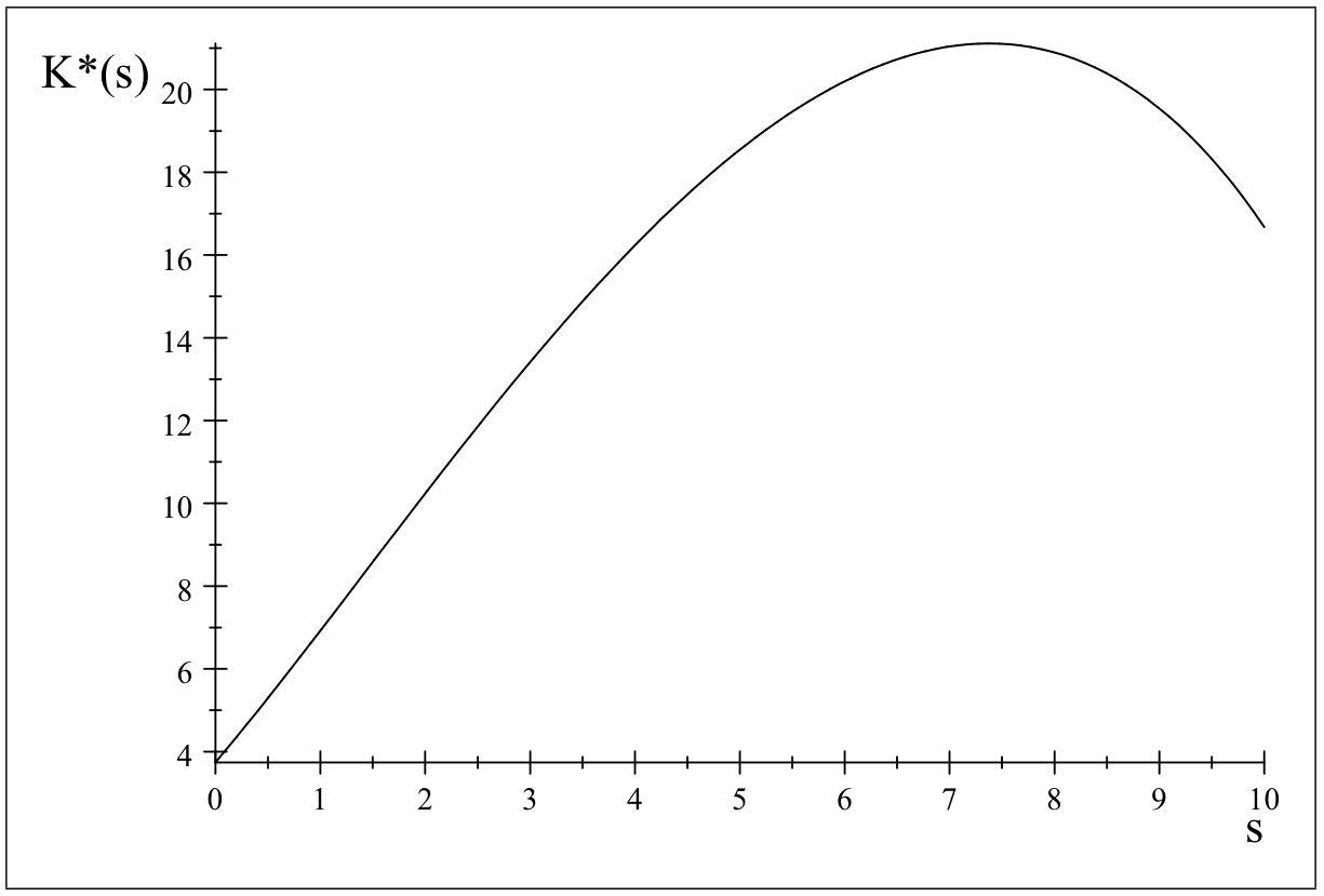 Figure 1
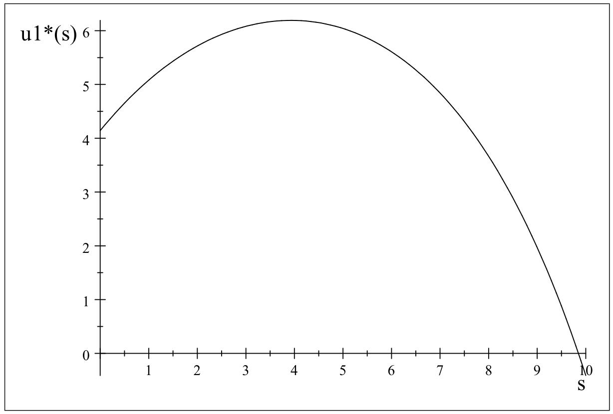 Figure 2
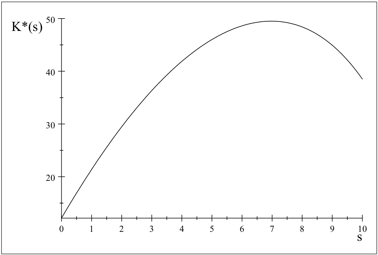 Figure 3
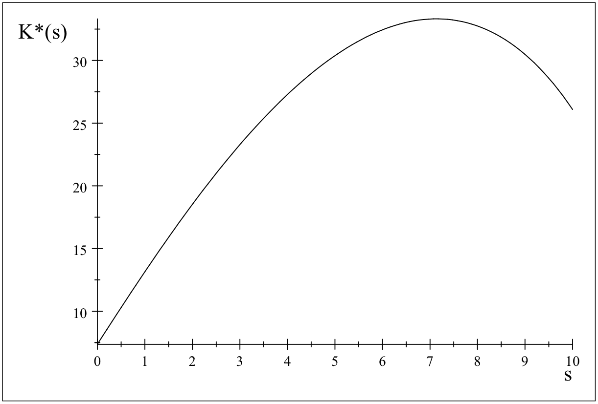 Figure 4
Peer Reviews
No public reviews on file for this paper yet. If you reviewed it on a platform where reviews are public (OpenReview, ICLR, NeurIPS, ICML), you can paste yours below so the community can read it here.
Videos
No videos yet. Explain this paper in a talk, walkthrough, or lecture? Add one.
Optimal Investment with
Vintage Capital:
Equilibrium Distributions
Silvia Faggian [1]
[1]S. Faggian, Department of Economics, Universitá “Ca’ Foscari” Venezia, Italy. [email protected].
,
Fausto Gozzi [2]
[2] Dipartimento di Economia e Finanza, Universitá LUISS - “Guido Carli, I-00162, Roma, Italy. [email protected].
and
Peter M. Kort [3]
[3] CentER, Department of Econometrics & Operations Research, Tilburg University, P.O. Box 90153, 5000 LE Tilburg, The Netherlands; Department of Economics, University of Antwerp, Prinsstraat 13, 2000 Antwerp 1, Belgium, [email protected].
Abstract.
The paper concerns the study of equilibrium points, or steady states, of economic systems arising in modeling optimal investment with vintage capital, namely, systems where all key variables (capitals, investments, prices) are indexed not only by time but also by age . Capital accumulation is hence described as a partial differential equation (briefly, PDE), and equilibrium points are in fact equilibrium distributions in the variable of ages. Investments in frontier as well as non-frontier vintages are possible. Firstly a general method is developed to compute and study equilibrium points of a wide range of infinite dimensional, infinite horizon boundary control problems for linear PDEs with convex criterion, possibly applying to a wide variety of economic problems. Sufficient and necessary conditions for existence of equilibrium points are derived in this general context. In particular, for optimal investment with vintage capital, existence and uniqueness of a long run equilibrium distribution is proved for general concave revenues and convex investment costs, and analytic formulas are obtained for optimal controls and trajectories in the long run, definitely showing how effective the theoretical machinery of optimal control in infinite dimension is in computing explicitly equilibrium distributions, and suggesting that the same method can be applied in examples yielding the same abstract structure. To this extent, the results of this work constitutes a first crucial step towards a thorough understanding of the behavior of optimal controls and trajectories in the long run.
Key words: Equilibrium Points; Equilibrium Distributions; Vintage Capital Stock; Age-structured systems; Maximum Principle in Hilbert spaces; Boundary control; Optimal Investment.
Journal of Economic Literature: C61, C62, E22
Contents
1. Introduction
Computing equilibrium points, or steady states, and describing their properties is one of the main goals in the mathematics of economic models. This task, when presuming an underlying optimal control problem with infinite horizon, is already nontrivial with one state variable, but it becomes harsh when the dynamics of the system are infinite dimensional, like in cases when heterogeneity/path dependency is taken into account. This is the case, for instance, of optimal investment with vintage capital (capital stock is heterogeneous in age, see e.g. [50, 35]), of spatial growth models (capital stock is heterogeneous in space, see e.g. [18, 34, 19]), of growth models with time-to-build (capital stock is path dependent, see e.g. [5, 6, 7]), or of models with heterogeneous agents (see e.g. [67]). In all these examples, equilibrium points are indeed functions (of vintage, or space, or age) and may be more properly referred to as “equilibrium distributions”. Up to now such equilibrium distributions have been studied only when the value function of the control problem is described by an analytic formula – a requirement which is very seldom met – so that many interesting cases are left out of the picture.
On the contrary, this work addresses the study of equilibrium distributions in cases where no explicit formula for the value function is available, moreover it does so under the general assumptions of an infinite-horizon infinite-dimensional control problem with linear state equation and general convex (concave, in the application) payoff, providing a theoretical tool that can be used in a variety of applied examples. In fact, the theory is put immediately into practise for the optimal investment model with vintage capital, obtaining analytic formulas for the equilibrium distributions, and a complete sensitivity analysis for some instances of the problem. Hence the paper contains a theoretical and an applied part, both of equal weight and dignity, whose main achievements are listed below.
For the general theory (Sections 2, 3 and 4), we reprise and complete the study of the control problems analysed in Faggian and Gozzi [44]. 111Note that in this theoretical context, since equilibrium distributions can be seen as points in a suitable infinite dimensional vector space, a space of functions, they will be still named “equilibrium points” There Dynamic Programming (DP) was employed to prove the existence and uniqueness of a regular solution of the Hamilton-Jacobi-Bellman (HJB) equation, as well as a verification theorem implying existence and uniqueness of optimal feedback controls, and the fact that coincides with the value function. Overall and differently from most contributions to the subject, this work presents an integrated approach between the DP and MP methods of optimal control theory. In particular:
- (a)
a co-state is associated to the state variable, and necessary and sufficient conditions for the optimal path are established in the form of a Maximum Principle (MP) (Theorem 4.5);
- (b)
the co-state associated to an optimal state is shown to coincide with the spatial gradient of the value function evaluated at that optimal state (Theorem 4.6);
- (c)
the definition of two types of equilibrium points is introduced: the stationary solutions of the state-costate system, called MP-equilibrium points, and the stationary solutions of the closed loop equation (CLE) arising in the DP approach (Definition 4.8), called CLE-equilibrium points;
- (d)
the relationship between the two types of equilibrium points is explained, and sufficient (and necessary) conditions for existence of such equilibria are provided (Theorem 4.10);
- (e)
two results on the stability of CLE-equilibrium points are given by using or adapting the existing literature (Propositions 4.15 and 4.16).
It is important noting that the theory cannot be used straightforwardly to treat applied problems in a satisfactory way. This happens on the one hand because the results in infinite dimension need to be translated into terms of the application under analysis, and on the other hand as it may be necessary to exploit the particular structure of the applied problem to specify formulas for practical use. One example is worked out through Theorem 5.5, in the case of the model of optimal investment with vintage capital.
In the applied part of this work (Sections 5 and 6), the theoretical results are used on the optimal investment model with vintage capital deriving:
- (e)
the existence of MP- or CLE-equilibrium points, which is proven equivalent to the existence of solutions of a numerical equation explicitly derived from the data;
- (f)
analytic formulas for MP- or CLE-equilibrium points in some relevant examples;
- (g)
a sensitivity analysis for some particular sets of data.
In particular, the sensitivity analysis enables the development of new economic results while analyzing the vintage capital stock model in which revenue is a strictly concave and linear quadratic function of output, where the strict concavity is caused by market power on the output market. As is standard in this literature (Feichtinger et al. [50]), output linearly depends on the capital goods, whereas investment costs are convex and linear quadratic. We show that the equilibrium distribution capital stock is first increasing and then decreasing in the age of the capital good. The increasing part is the result of investment costs being relatively large when capital goods are relatively new. On the other hand, such investments are attractive due to the long lifetime of new capital goods. Capital goods of older age have a shorter lifetime. This gives an incentive to reduce investments in older capital goods, resulting in the fact that the equilibrium distribution capital stock for old machines decreases with respect to age. We further establish another non-monotonicity dependence of the equilibrium distribution capital goods level, but now with respect to the productivity of the capital goods. If productivity is relatively low, the number of capital goods increases if productivity goes up. This is because a given capital good produces more so that the firm is more eager to invest in it. On the other hand, if productivity is relatively large the firm decreases investments, because otherwise the firm overproduces resulting in a too low marginal revenue. In other words, some optimal output level exists and less capital goods are needed to produce this level when productivity is high.
In conclusion, this work shows how successfully and effectively the theoretical machinery of optimal control in infinite dimension is in computing explicit formulas and studying properties for equilibrium distributions, also in absence of an explicit formula for the value function. We believe that the theoretical tools developed in the first part of this work can be successfully employed in examples yielding the same abstract structure (like those mentioned at the beginning of this introduction) and possibly extended to more complex cases with the use of suitable numerical approximations: this will be the subject of future work.
The paper is organized as follows. Section 2 presents a family of optimal investment models with vintage capital. Sections 3 presents the abstract optimal control problem and shows that the problem contained in Section 2 falls into that wider class. Section 4 is the theoretical core of the paper, where we recall the results obtained with the DP approach in [44] (Section 4.1), we state and prove first order optimality conditions in terms of a Maximum Principle (Section 4.2), and we present and discuss the general results on equilibrium points (Section 4.3). In Section 5, the general results of the previous sections are applied to the model of optimal investment with vintage capital, providing a technique to derive analytic formulas for the equilibrium distributions. Finally, in Section 6, a sensitivity analysis is conducted on some instances of the problem of Section 5, i.e. where both revenues and costs are chosen linear-quadratic. This section also contains numerical results as illustration. An appendix with proofs of the theorems of Section 4 and 5, as well as some additional results, completes the work.
We remark that he paper is organized as to allow the reader less interested in mathematical details to approach Sections 5 and 6 without necessarily going through the theoretical Sections 3 and 4.
1.1. Literature Review
We complete this introductory section with an overview of literature on vintage capital, and on optimal control of infinite dynamical systems, thereby explaining what the present paper adds to each field.
From an economic point of view, the paper contributes to the literature of vintage capital stock models. Such models extend standard capital accumulation models, like, among many others, Eisner and Strotz [32] and Davidson and Harris [29] where capital goods are a function of just time. The extension is that also the age of the capital goods is taken into account. This enables to distinguish different vintages of capital goods so that one could explicitly analyze issues like aging (Barucci and Gozzi [14]), learning (Greenwood and Jovanovic [57]), pollution (Xepapadeas and De Zeeuw [72]), forest management (Fabbri, Faggian and Freni [37]), and technological progress (Feichtinger et al. [50]). We consider the kind of vintage capital stock models where investments in older capital goods are possible. This distinguishes the framework to be considered from works like Solow et al.[69], Malcomson [65], Benhabib and Rustichini [16], and Boucekkine et al. [20, 21, 22, 23].
The first contribution in vintage capital literature, which consider models where investments in older capital goods are also possible, is Barucci and Gozzi [15]. They consider the vintage capital stock framework where, as in Feichtinger et al. [49], revenue is linearly increasing in output, implying that the output price is constant, and linear-quadratic investment costs. Like in Feichtinger et al. [49], they do derive equilibrium distribution expressions for capital goods of different ages and corresponding investments. The present paper generalizes these contributions by obtaining the equilibrium distribution expression of the capital goods for a model with general concave function.
Barucci and Gozzi [14] extends Barucci and Gozzi [15] by considering technological progress, while in Xepapadeas and De Zeeuw [72] the production process produces emissions next to products. Both papers keep the revenue linearly dependent on output. Provided an equilibrium distribution exists, which is not the case when we have ongoing technological progress as in Barucci and Gozzi [14], due to this linearity equilibrium distribution expressions are much easier to obtain compared to a revenue function being concave as in the present paper.
Closer to our present paper than the works cited above is Feichtinger et al. [50], in which also a firm with market power is considered. The difference with our work is that Feichtinger et al. considers technological progress. In particular, the main part of their work analyzes how the firm reacts with its investment policy to a technological breakthrough, which is a point in time at which a new technology is invented. The implication is that productivity of the capital goods of vintages borne after the breakthrough time jumps upwards. Our model is simpler in the sense that we do not consider technological progress. However, our analysis goes further than in Feichtinger et al. [50] in that we were able to derive an analytical expression for the equilibrium distribution. This we could do for a general concave revenue function, where Feichtinger et al. [50] just considers linear-quadratic revenue. Note that after the technological breakthrough Feichtinger’s model turns into our model with prespecified revenue function. This implies that also in their framework a unique equilibrium distribution exists, which can be calculated using the results of the present paper.
From the point of view of mathematics, the main features of the optimal control problem here considered are: the linear state equation and the convex cost criterion; the presence of a boundary control; the age structure of the driving operator in the state equation.
Optimal control of infinite dimensional systems is the subject of many books and papers in the recent literature. Among the books in the deterministic case we mention Lions [62] and Barbu and Da Prato [9], and the more recent ones Li and Yong [63], and Troltzsch [71]. For the stochastic case (concerning the dynamic programming approach) one can see the recent book [36].
Concerning the dynamic programming approach to problems with linear state equation and convex cost but with distributed control, we refer the reader to Barbu and Da Prato [9, 10, 11], for some linear convex problems to Di Blasio [30, 31], for the case of constrained control to Cannarsa and Di Blasio [24], and for the case of state constraints to Barbu, Da Prato and Popa [12] (see also Gozzi [51, 52, 53] for a generalization of this approach to the case of semilinear state equations). For boundary control problems we recall, in the case of linear systems and quadratic costs (where the HJB equation reduces to the operator Riccati equation) e.g. the books by Lasiecka and Triggiani [60, 61], the book by Bensoussan, Da Prato, Delfour and Mitter [17], and, for nonautonomous systems, the papers by Acquistapace, Flandoli and Terreni [1, 2, 3, 4]. For the case of a linear system and a general convex cost function, we mention the papers by Faggian [38, 39, 40, 41, 42], and by Faggian and Gozzi [43, 44] (in particular, the theory developed in the last two works is the starting point for theory in the present paper, and is recalled in Section 4.1). On the Pontryagin maximum principle for boundary control problems we mention again, in the linear quadratic case, the books [60, 61, 62] and [17]; in the case of linear systems with convex cost, e.g., the book by Barbu and Precupanu (Chapter 4 in [13]), and the papers [8], [58]; for general nonlinear boundary control problems, e.g., [27], [45], [46], [70] [55] [56]. None of them covers the class of problems treated here.
The main contributions of the present paper with respect to the mathematical literature quoted above are: (1) the proof of the Maximum Principle for infinite dimensional, infinite horizon optimal control problems with features ; (2) the co-state inclusion which reconnects the value function with the co-state; (3) the analysis of equilibrium points of the control problem.
2. The optimal investment model with vintage capital
We now describe the model of optimal investment with vintage capital, in the setting introduced by Barucci and Gozzi [15][14], and later reprised and generalized by Feichtinger et al. [48, 49, 50], and by Faggian [40, 41] and Faggian and Gozzi [43].
The capital accumulation process is given by the following system
[TABLE]
with the initial time, the maximal allowed age, and with horizon . The unknown represents the amount of capital goods of age accumulated at time , the initial datum is a function (the space of square integrable functions on ), is a depreciation factor. Moreover, is the investment in new capital goods ( is the boundary control) while is the investment at time in capital goods of age (hence, the distributed control). Investments are jointly referred to as the control . The output rate is
[TABLE]
where is a productivity parameter. Selling the output to consumers results in an instantaneous revenue, where is a concave function. Capital stock can be increased by investing, and investment costs are given by
[TABLE]
with indicating the investment cost rate for technologies of age , the investment cost in new technologies, including adjustment costs, , convex in the control variables. The firm’s payoff is then represented by the functional
[TABLE]
where is the discount rate. Note that is usually assumed positive, but here we leave the possibility of choosing a negative (corresponding, for example, to a negative interest rate). The entrepreneur’s problem is that of maximizing over all state–control pairs which are solutions (in a suitable sense) of equation (2.1) and keep the capital stock nonnegative at all times. Such a problem is known as vintage capital problem, for the capital goods depend jointly on time and on age , which is equivalent to their dependence on time and vintage .
We finally recall the definition of the value function of the problem
[TABLE]
Since and are not time dependent it is immediate to see that
[TABLE]
Remark 2.1**.**
As a matter of fact, we treat the above problem without the state constraints for all and , and check that constraints are satisfied a posteriori by the optimal trajectories of the unconstrained problem. In such a case, those trajectories are also optimal for the problem with state constraints.
2.1. Revenues and costs
In order to be able to treat optimal investment with vintage capital into the wider class of abstract problems described in Sections 3 and 4, we specify the assumptions on revenues and costs which ensure that the basic assumptions of the abstract problem (Assumptions 3.2, (3)-(6)) are fulfilled.
Assumptions 2.2**.**
- ()
, concave, Lipschitz continuous. Moreover 222 is the space of square integrable functions which admit a square integrable derivative in weak sense. Continuous functions with piecewise continuous derivatives are included in this space. and . 2. ()
and are convex, lower semi–continuous functions, with injective333A multivalued function is injective when for every , . subdifferential at all . 3. ()
(are Fréchet differentiable and) have Lipschitz continuous derivatives, for all . 4. ()
and are bounded below by a function of type , for some , , .
In the above statement, we denoted by the convex conjugate of a convex function , in particular Note that no strong regularity of is required.
For example, suitable choices for the revenues are the following:
(a) Linear-quadratic: ;
(b) Logarithmic: for and for ;
(c) Power : with ( arbitrary small), for and for Note in particular that this converges as tends to 0 to for and for 444The definition of for negative values of is needed in order to apply the general theory, although negative values of will never emerge in our calculations. Note also that setting for is equivalent to require in optimal solutions.
Suitable choices for the costs are, once set , with , , the following:
(A) Linear-quadratic:
[TABLE]
(B) Linear+quadratic with constrained control:
[TABLE]
where
[TABLE]
Such a cost can be easily generalized to a case where belongs to any compact interval and not necessarily .
(C) Linear+Power costs:
[TABLE]
where, for ,
[TABLE]
which implies also positivity constraints of the controls.
We treat all of these cases in Section 5. Moreover, in Section 6 we treat the case of linear–quadratic revenues and costs for which we derive analytic formulas for the long run optimal couples, and perform a complete sensitivity analysis.
The reader is advised that Sections 3, 4, and the Appendix are devoted to the mathematics of the general problem and require a good knowledge of functional analysis to be fully understood. Nonetheless, they may be skipped at a first reading, as the reader will find in Section 5 the theoretical results translated in terms of the problem of optimal investment with vintage capital.
3. The theoretical framework
Here we introduce an abstract class of infinite dimensional optimal control problems with linear evolution equation and convex payoff, in which the control may also act on the boundary, and address it as (P). Then, in Section 3.3 we show that the optimal investment model with vintage capital described in the previous section is of type (P).
3.1. Notation
The expression means the maximum of the real numbers and . If is a Banach space, we indicate its norm with , its dual with , with the duality pairing. When we use for simplicity in place of . If is also a Hilbert space, we indicate with the inner product in .
If and are Banach spaces, then denotes all Fréchet differentiable functions from to , and the set of all linear and continuous operators from to , with associated norm . Moreover we set
[TABLE]
and, for ,
[TABLE]
Note that are Banach spaces if endowed with the norm , so that continuity is intended with respect to such norms. Furthermore, we set
[TABLE]
Finally, if is a Hilbert space and is a convex function, then will denote its convex conjugate, namely , .
3.2. The abstract optimal control problem (P)
We consider two real separable Hilbert spaces and with continuously embedded in . We identify with its dual and we call the topological dual of , which we do not identify with for the reasons explained in Section 3.3. We then get a so-called Gelfand triple
[TABLE]
We choose as state space. The control space is the real separable Hilbert space (which we identify with its dual ). We consider the control system with state space , control space , and varying initial time , described by
[TABLE]
where and are linear operators, possibly unbounded. Moreover, we take a convex functional of the following type
[TABLE]
where the function and are convex functions. The problem (P) is that of minimizing with respect to , over the set of admissible controls
[TABLE]
which is a Banach space with the norm
[TABLE]
Remark 3.1**.**
In the above problem no constraints on controls or on states are assumed although, in economic applications, the state represents capital stock, usually assumed nonnegative. Here we proceed along with the frequently used idea (see e.g.[35]) to check ex post that the constraints are satisfied by the optimal trajectories of the unconstrained problem, so those trajectories are optimal also for the constrained problem.
The basic assumptions on the data are stated below and will hold throughout the paper.
Assumptions 3.2**.**
- (1)
is the infinitesimal generator of a strongly continuous semigroup on . Moreover there exists such that555When , a semigroup with this property is usually called a pseudo-contraction semigroup, as is a contraction semigroup with generator .
[TABLE] 2. (2)
; 3. (3)
4. (4)
is convex and lower semi–continuous, is injective. 5. (5)
, ; 6. (6)
, , : , ; 7. (7)
.
In proving some results we will need to specify the assumption (7) above as follows.
Assumptions 3.3**.**
In addition to Assumption 3.2, we require that either
- (1)
or
- (2)
The adjoint of in the inner product of is denoted by , while the adjoint of with respect to the duality in is the unbounded operator on ,
Remark 3.4**.**
We recall that, if a function is lower semicontinuous and convex (and not identically ), then the subgradient is defined as Moreover if is injective then is Fréchet differentiable with for all .
3.3. Optimal investment with vintage capital is of type (P)
We end the section by showing that the problem of optimal investment with vintage capital described in Section 2 falls in the general class (P) described above and refer interested readers to [41] for full detail.666See also [33], [17] or [68] for the general theory of strongly continuous semigroups and evolution equations.
We at first formulate an intermediate abstract problem in , the space of square integrable functions of variable , using the modified translation semigroup on , namely the linear operators such that
[TABLE]
If then the generator of is the operator with
[TABLE]
The adjoint of is then with
[TABLE]
generating itself a modified translation semigroup on given by
[TABLE]
The control space is , the control function is a couple
[TABLE]
and the control operator is given by
[TABLE]
being the Dirac delta at the point [math]. With this notation, the original state equation (2.1) can be written as
[TABLE]
Note that and are Hilbert spaces, and that is unbounded, meaning that it is not a continuous operator from to (unless , corresponding to identically null boundary control ), for the Dirac delta does not lie in . Then (3.4) needs to be interpreted in a suitable way, for instance in an extended state space.
Then we generalize all previous notions to a wider space. We set and assume as state space of the abstract problem. Indeed by standard arguments (see e.g. [33, Section II.5]) – and in particular by replacing the scalar product in with the duality pairing with , (coinciding with the inner product in when ) – the semigroup can be extended to a strongly continuous semigroup on , by setting
[TABLE]
The generator of is the operator with . Moreover the semigroup can be restricted to a strongly continuous semigroup on , with generator the restriction of to . Such restriction is exactly the adjoint of in the duality and is then denoted, as in the previous subsection, by .
The role of is that of pivot space between and , namely , with continuous inclusions. The control operator is then in . Its adjoint is given by
[TABLE]
It is also useful to note that is well defined and that
[TABLE]
The target functional is also interpreted on extended spaces once the production function is described as
[TABLE]
where, the duality pairing between and has replaced the scalar product in in the original definition (2.2) of , and Then (2.4) becomes
[TABLE]
The firm’s optimal investment problem falls into the wider class described in the next theoretical sections, provided it is reformulated as a minimization problem, where the functions and there described are chosen as
[TABLE]
Indeed the following Lemma holds true.
Lemma 3.5**.**
Assumptions 2.2 imply, along with the above definitions of and and (3.9), that Assumptions 3.2 are satisfied with . Furthermore if , then Assumption 3.3 (1) is satisfied. If instead if and has at most linear growth, Assumption 3.3 (2) is satisfied.
Proof. Assumption 3.2-(1) is satisfied with since, for every we have, by definition of
[TABLE]
Assumption 3.2-(2) is trivially satisfied as pointed out above in the definition of . By Assumption 2.2, and is a Fréchet differentiable convex function of , with Fréchet differential defined by . Such differential is a Lipschitz continuous function of , with Lipschitz constant , as
[TABLE]
so that Assumption 3.2-(3) holds true. Assumptions 2.2() coupled with Remark 3.4 implies both Assumptions 3.2 (4) and that is convex and Fréchet differentiable. The fact that has Lipschitz differential is implied by (), so that also (5) holds true. Clearly () implies (6). The last statement is straightforward.
Remark 3.6**.**
It is important to note that, in the case when the functions and are both quadratic, neither (1) nor (2) are satisfied in Assumption 3.3. Nonetheless necessary and sufficient conditions of optimality (see Theorem 4.5) hold true, and the value function results regular (see Remark 4.4 and Section 5.2.1 for details).
4. Equilibrium points
Although the core of the section is the definition of equilibrium points of the abstract problem (P) and the investigation of their properties, some results are needed beforehand. Those obtained via Dynamic Programming, and contained in [44], are recalled for the reader’s convenience in Section 4.1. On the other hand, Section 4.2 contains new material, and in particular a version of the Maximum Principle for problem (P). Finally Section 4.3 contains the analysis of equilibrium points.
4.1. Dynamic Programming for problem (P)
We here recall the main results contained in [44]. If the value function is defined as
[TABLE]
and, if one sets , then , so that the Hamilton–Jacobi–Bellman equation associated to the problem by means of Dynamic Programming reduces to that with initial time , that is
[TABLE]
(with the unknown) whose candidate solution is . We refer to as to the Hamiltonian function.777Note that the function usually called Hamiltonian would be .
Definition 4.1**.**
A function is a classical solution of the stationary HJB equation (4.2) if it belongs to and satisfies (4.2) for every .
Theorem 4.2**.**
Let Assumptions 3.2 and 3.3 hold. Then there exists a unique classical solution to and it is given by the value function of the optimal control problem, that is
[TABLE]
Once we have established that is the unique classical solution to the stationary HJB equation, and since is Fréchet differentiable with Lipschitz derivative, we can build optimal feedbacks and prove the following theorem.
Theorem 4.3**.**
Let Assumptions 3.2 and 3.3 hold. Let and be fixed. Then there exists a unique optimal pair at . The optimal state is the unique solution of the Closed Loop Equation
[TABLE]
while the optimal control is given by the feedback formula
[TABLE]
where the optimal feedback map is Lipschitz continuous.
Remark 4.4**.**
There are relevant cases when Assumption 3.3 is not satisfied. One such example is the case, important for the applications, when costs and are quadratic (or linear + quadratic). Nonetheless Theorems 4.3 remains true, with identical proof to that provided in [44], if the value function is in . Indeed the regularity of implies that is a classical solution of the associated HJB equation (4.2) (to this extent see e.g. [63], ch. 6, Proposition 1.2, p. 225). In the case of quadratic costs, for instance, one proves that is itself quadratic, and hence in . Note also that if is not differentiable, then the closed loop equation (4.3) holds in the weaker sense of (4.8), as specified in the next section.
4.2. Maximum Principle for Problem (P)
The results contained in this section, namely Theorems 4.5 and 4.6, are new to literature and add to the theory developed in [38, 40, 41, 43, 44]. They establish a Maximum Principle for the problem at hand, and connect it to the results on Dynamic Programming contained in those papers. The reader may find all of the proofs in the Appendix, as well as some additional results. We advise the reader that, differently from [44] and in view of Remark 4.4, the new results are proved avoiding Assumption 3.3. As a consequence, if on the one hand the regularity of the value function of (P) does not necessarily hold true, on the other hand we are able to treat the case of the limit exponent , and hence of quadratic costs and , so important for the applications.
In order to establish a maximum principle, we first need to define a dual system associated to the mimimization problem. For all fixed and , we consider the equation
[TABLE]
where (the dual variable, or co-state of the system) is the unknown, and is the trajectory starting at at time and driven by control , given by (3.1). We assume such equation is also subject to the following transversality condition
[TABLE]
When necessary, we denote any solution of (4.4)(4.5) also by or by to remark its dependence on the data.
Heuristically speaking, the candidate conditions of optimality associated to the problem are the following:
[TABLE]
The ODEs for and appearing in (4.6) are intended, as it is usual in these cases, in mild sense, see Definition A.1 in Appendix A. Moreover, by conjugation formula, we have
[TABLE]
We refer to (4.7) as to maximum condition. It has to be satisfied for a.a. .
The conditions listed in (4.6) prove to be necessary and sufficient for optimality for all , in the sense specified next.
Theorem 4.5**.**
(Maximum Principle).* Let Assumptions 3.2 be satisfied. Let and . Let , .*
Let be a given admissible pair at . If there exists a function satisfying, along with and , the system then is optimal at for the problem of minimizing .
*Assume further that, either and , or , and . Then the viceversa of (i) holds, i.e., any couple optimal at necessarily admits a costate satisfying, along with and , system *
The next theorem containes the so-called co-state inclusion. Note that the case of is discussed separately, as the value function is not necessarily Fréchet differentiable (unless Assumption 3.3 holds or ad hoc regularity results are given).
Theorem 4.6**.**
(Co-state inclusion).* In Assumptions 3.2, for , suppose that either , or and . Let be optimal at , and let be the associated co-state. Let also be the value function of problem (P). Then*
[TABLE]
where is the subdifferential of the convex function . If in addition , then and coincides with , so that
[TABLE]
Remark 4.7**.**
Note that, for and , and by making use of Theorem 4.5, and of equations (4.6) and (4.7), one obtains
[TABLE]
so that the general version of the closed loop equation (4.3) becomes a differential inclusion
[TABLE]
also to be intended in mild sense.
4.3. Equilibrium points
We give two different definitions of equilibrium points for problems (P), and later show to which extent they are equivalent.
Definition 4.8**.**
A MP-equilibrium point of problem is any stationary solution of . This is equivalent to require that belongs to and satisfies
[TABLE]
A CLE-equilibrium point of problem is any that is a stationary solution of the closed loop equation (4.8). This is equivalent to require and
[TABLE]
Remark 4.9**.**
When and , then (4.9) is equivalent to
[TABLE]
and (4.10) is equivalent to
[TABLE]
As a consequence of Remark 4.4, the equations (4.8), (4.10) and (4.12) hold as equalities with in place of when Fréchet differentiable in (e.g. when , or when regularity can be proven separately).
The proof of the equivalences in the above definition is straightforward as they are based on standard regularity of convolutions of semigroups. We omit them for brevity.
We have the following result.
Theorem 4.10**.**
Let Assumptions 3.2 be satisfied, , .
Let be any MP-equilibrium point. Then the constant control is optimal at and
[TABLE]
moreover is a CLE-equilibrium point and
[TABLE]
Let be a CLE-equilibrium point, . Let either , or and . Assume that is Fréchet differentiable in . Then , where
[TABLE]
is an MP-equilibrium point, the control is optimal at (0,{\color[rgb]{0,0,1}\hat{x}}) and .
One important consequence of the above theorem is that it provides the following equation for a CLE-equilibrium point (or for the first component of an MP-equilibrium point)
[TABLE]
In addition, whenever (this assumption is satisfied in the optimal investment problem with vintage capital described in Section 2) solutions of (4.15) can be regarded as fixed points of the operator , defined by
[TABLE]
For the applications, the most efficient way of making use of such relations is to rewrite them in terms of the specific sets of data, and compute when possible the optimal equilibrium distributions. In particular, in Section 5 we will see how (4.16) is interpreted in terms of the data of optimal investment with vintage capital, so that fixed points of may be directly computed by solving a numeric equation.
However, in the general case, it is possible to provide sufficient conditions for the existence and uniqueness of a fixed point of the operator using well known fixed point theorems although, as one expects, such conditions may hardly be very sharp. To this extent, we provide here only Lemma 4.11, which is a straightforward application of the contraction mapping principle.
Lemma 4.11**.**
Let Assumptions of Theorem 4.10 be satisfied. Assume moreover that
[TABLE]
Then there exists a unique solution to the equation (4.16).
Remark 4.12**.**
The operator above is considered as an operator from to itself. Since its image is contained in , when looking for fixed points, it is also equivalent to look at it as an operator from to itself, considered as a subspace of , as done in Lemma 5.4.
Remark 4.13**.**
All above results could be generalized to the case in which we have state constraints and the function is convex but not necessarily Fréchet differentiable. This could be done using the results of [42] and generalizing them to the infinite horizon case, using the same arguments in [53]. Clearly, at points where is not Fréchet differentiable, one would have to choose an element of the subdifferential of .
4.4. Stability
Once existence (and possibly uniqueness) of equilibrium points is proven, it is possible to study their stability properties adapting known results such as those in [59] or in chapter 9 in [64], or by direct proof, as we see next. In all cases, stability will be proven with respect to the topology of . For the reader’s convenience we recall the definition here below.
Definition 4.14**.**
A CLE-equilibrim point is stable in the topology of if, such that, if and is the optimal trajectory starting at , then . If in addition then is asymptotically stable. Finally, if the same property hold true for all , then is globally asymptotically stable.
The first criterium to establish stability is contained in the following proposition and makes use of the linearization method. The proof follows from Corollary 2.2 in [59].
Proposition 4.15**.**
(Stability by linearization)* Let Assumption 3.2 be satisfied and . For set , and assume that is a CLE-equilibrium point for (P), that is continuously Fréchet differentiable at a neighborhood of , and denote by the spectrum of the operator . If , then is stable in the topology of . Moreover, it is also asymptotically stable in the topology of . If , is unstable in the topology of .*
Another result that can be used is the following. Recall that indicates the inner product in .
Proposition 4.16**.**
(Stability by dissipativity)* Let Assumption 3.2 be satisfied and let . For , and , and assume that, when , the solution of the closed loop equation*
[TABLE]
belongs to for all . Let be a CLE-equilibrium point for (P). Assume that is dissipative near , i.e. there exists an open ball in centered at , and such that, for every ,
[TABLE]
Then is stable in the topology of . If then is asymptotically stable in the topology of . If is dissipative on the whole and then is globally asymptotically stable.
Corollary 4.17**.**
Let the assumptions of Proposition 4.16 be verified, except (4.18). Let the operator satisfy , for all in , with a fixed constant. If there exists a neighborhood of where is Lipschitz continuous (in the topology of ) with Lipschitz constant strictly smaller than , then is asymptotically stable in the topology of . If is Lipschitz continuous in with Lipschitz constant strictly smaller than then is globally asymptotically stable.
In particular, the above corollary may be applied to the examples in Section 5, see e.g. subsection 5.2.1.
5. Application to Optimal Investment with Vintage Capital
The aim of this section is to show how valuable our general theory can be when analyzing specific applications, and in particular when trying to derive analytic formulas for equilibrium distributions. This process unfolds by computing MP-equilibrium/CLE-equilibrium points for that problem rephrased in abstract form as in Section 3.3.
We begin by noting that the value function of the optimal control problem described in Section 2 (see (2.5)), satisfies, as a consequence of (2.4), (3.9) and (4.1),
[TABLE]
where is the value function, defined in Section 4.1, of the abstract problem (P) for . Note that is a concave function, as is convex. Note also that, under additional assumptions (e.g. Assumption 3.3, or regularity assumptions on ), is the unique classical solution of HJB equation (4.2) in the sense of Definition 4.1. As a consequence, the natural co-state for the maximization problem would be
[TABLE]
with the co-state of the abstract problem whose properties are described in Theorem 4.5 and 4.6. Then the optimality conditions (4.6) for a triplet can be written as the following set of equations
[TABLE]
[TABLE]
[TABLE]
[TABLE]
Note that (5.1) and (5.2) are derived from (4.6) by making use of (4.7) and (A.15), while (5.4) is well known and can be obtained by means of characteristics method (see e.g. [14]).
The following proposition is an immediate consequence of Theorem 4.5 and of Lemma 3.5.
Proposition 5.1**.**
Under Assumptions 2.2, with and , the optimality conditions (5.1)(5.2)(5.4) are necessary and sufficient for a couple to be optimal at for the problem of optimal investment with vintage capital described in Section 2.
5.1. Characterization of Equilibrium Points
It is natural to define an equilibrium point for the problem consistently with Section 4.3. For the reader’s convenience, Definition 4.8 is reformulated below in terms of the problem of optimal investment with vintage capital.
It is important to note that an equilibrium point is actually a function of the variable (although independent of ) dependent on the variable , hence an equilibrium distribution.
Definition 5.2**.**
In reference to the the optimal investment problem with vintage capital:
a MP-equilibrium point is a stationary solution of the system of equations ;
for Fréchet differentiable, a CLE-equilibrium point is any which is a stationary solution of equation (5.4) when
[TABLE]
Remark 5.3**.**
Several remarks are here due.
- (1)
Theorem 4.10 implies, in the assumptions of Proposition 5.1 that and are equivalent in the following sense: the first component of a MP-equilibrium point is also a CLE-equilibrium point; conversely, when is Fréchet differentiable, a CLE-equilibrium point can be used to build a MP-equilibrium point by means of , having as first component. 2. (2)
If is not Fréchet differentiable, the closed loop equation (as well as the definition above) may be generalized to a differential inclusion in the sense of (4.8), where is replaced by the superdifferential . 3. (3)
Definition 5.2 is consistent with Definition 4.8 as here and .
We further characterize MP-equilibrium/CLE-equilibrium points as fixed points of a suitable operator. To this extent we define
[TABLE]
i.e. is the discounted return associated with a unit of capital of vintage .
Lemma 5.4**.**
Under Assumptions 2.2, is a CLE-equilibrium point if and only if it is a fixed point of the operator defined by
[TABLE]
that is, if and only if for a.e. in . Moreover where
[TABLE]
is a MP-equilibrium point.
The proof of the lemma is contained in Appendix C.
Note that solving the equation within a space of functions is not particularly handy. Nonetheless solving such functional equation is equivalent - and in the generality of cases - to solving a numeric equation. In this sense, the following theorem contains the most interesting result of the section.
Theorem 5.5**.**
Let Assumptions 2.2 be satisfied, and let be given by (5.6). Moreover, for any and , consider the function
[TABLE]
Then is a solution of , if and only if
[TABLE]
with a solution in of
[TABLE]
The proof of the theorem is contained in Appendix C.
Remark 5.6**.**
Note that the solution of (5.10) is unique and nonnegative when, for instance, Indeed is decreasing and and are convex functions, then the right hand side of (5.10) is a positive decreasing function of . Hence the function
[TABLE]
satisfies , is strictly increasing to , and hence has exactly one nonnegative zero.
Note that (5.6) and (5.9) are general formulas, holding for any choice of costs and revenues, as long as they satisfy Assumptions 2.2. More explicit formulas for the optimal equilibrium distribution may be derived once costs and revenues are further specified.
5.2. Linear-quadratic costs
Now we make formulas more explicit in the case of cost functions satisfying . We derive
[TABLE]
so that
[TABLE]
In this case, (5.6) becomes
[TABLE]
where and are the positive functions
[TABLE]
[TABLE]
If in addition we define the positive coefficients
[TABLE]
then the following result follows as a consequence of Theorem 5.5.
Corollary 5.7**.**
Let Assumption 2.2 and (2.7) be satisfied. Let , and be defined respectively by (5.14), (5.15) and (5.16). Then is a MP-equilibrium point if and only if is a solution of
[TABLE]
and
[TABLE]
and moreover and are given by (5.7). The constant control is optimal at {\color[rgb]{1.0,0.0,0.0}\bar{x}}, is also a CLE-equilibrium point and, if is Fréchet differentiable, then it is also the unique CLE-equilibrium point.
Remark 5.8**.**
If the CLE-equilibrium point identified by Corollary 5.7 is such that at all , then is also a CLE-equilibrium point for the problem with state constraints for all and (see also Remarks 2.1 and 3.1).
Remark 5.9**.**
Note that Assumptions 2.2 are satisfied here with , so that is not necessarily Fréchet differentiable. That implies that, although the first component of a MP-equilibrium point is also a CLE-equilibrium point, the viceversa may fail: there may be CLE-equilibrium points which do not derive as first components of a MP- equilibrium point, i.e. solutions of the stationary closed loop equation which fail to be optimal. For a further discussion on regularity of , the reader is referrred to Section 5.2.1.
Once is chosen, the results in Corollary 5.7 leads to an explicit formula for that CLE-equilibrium point, as illustrated in the next lemma.
Lemma 5.10**.**
In the assumptions of Corollary 5.7, there exists a unique CLE-equilibrium point , described by the formuals below, for the associated choices of the revenue :
- (i)
If , then
[TABLE] 2. (ii)
If for and for , then
[TABLE] 3. (iii)
If with , , for and for , then where is the unique positive solution of
[TABLE] 4. (iv)
If with , , for and for (case with state constraints) then where is the unique positive solution of
[TABLE]
Proof.
The proof follows from straightforward computations. ∎
5.2.1. Stability of Equilibrium Distributions
We close the section on linear-quadratic costs (2.7) by briefly discussing stability of equilibrium distributions and, in some subcases, the regularity of the value function, by applying the results contained in Section 4.4. The concept of stability here used is that of Definition 4.14, which is natural in this context. We remark though that the convergence of functions there mentioned (i.e. in the topology of ) is not a convergence in the space but, roughly speaking, the (weaker) convergence of their primitive functions.
Lemma 5.11**.**
In the assumptions of Corollary 5.7, suppose in addition that the value function is Fréchet differentiable, and set , where indicates the Lipschitz constant of the gradient . If (respectively, ) then is stable (resp., asimptotically stable) in the sense of Definition 4.14.
The proof of the lemma is contained in Appendix C.
Remark 5.12**.**
In particular, the previous Lemma applies when is of the type described in Lemma 5.10 . Indeed with some extra work one shows that in this case the value function of the abstract problem is of type
[TABLE]
for a suitable linear operator , and , where and are the spaces introduced in Subsection 3.3. Hence is differentiable with Fréchet differential , and (for a proof, we refer the reader to [60], vol 1, ch.2). This applies in particular to the linear-quadratic examples of Section 6.
5.3. Linear-quadratic costs, constrained control
We now choose costs as in . We then derive
[TABLE]
Note that is a function, with Lipschitz derivative
[TABLE]
As a consequence, the Legendre transform of is
[TABLE]
which is Fréchet differentiable with differential
[TABLE]
while the operator (5.6) is given by
[TABLE]
Remark 5.13**.**
Note that, with this choice of costs , Assumptions 2.2 are satisfied with so that, by Theorem 4.2, the value function is in . By Lemma 5.4 and Theorem 5.5 we then get that there exists a unique CLE-equilibrium point, coinciding with the first component of the unique MP-equilibrium point.
From this point on, one may procede as in the proof of Theorem 5.5 and Lemma 5.10 and compute CLE-equilibrium points, once the data are further specified.
5.4. Power costs
We now choose costs as in and set . Note that implies . The convex conjugate of the costs are then
[TABLE]
with Lipschitz derivative
[TABLE]
As a consequence the Legendre transform of is
[TABLE]
which is a function with Lipschitz differential
[TABLE]
Moreover
[TABLE]
Remark 5.14**.**
Note that Remark 5.13 applies also to this case.
6. Sensitivity analysis in two special cases
We here analyze further the case of linear-quadratic costs discussed in Section 5.2, and develop sensitivity analysis accordingly. In particular we assume
[TABLE]
Summing up, the objective functional of the profit maximizing firm is
[TABLE]
We study separately the cases oflinear-quadratic and power revenues, depicted respectively in Lemma 5.10 and .
6.1. Linear-Quadratic Revenues
We here assume
[TABLE]
as in Lemma 5.10 , so that the equilibrium distribution there described equals
[TABLE]
in which
[TABLE]
and
[TABLE]
where
[TABLE]
[TABLE]
The explicit expression for the equilibrium distribution capital stock for every age, allows us to obtain interesting economic implications. To illustrate, we establish some numerical results, which mostly are analytically proved as well. We start out from the following parameter values:
[TABLE]
The equilibrium distribution capital stock is depicted in Figure 1.
We see that capital goods are non-monotonic with respect to age. To understand this, Figure 2 depicts equilibrium distribution investment behavior, where investment is given by
[TABLE]
with being the production quantity in the equilibrium distribution.
Acquiring capital goods of older age is more attractive because they are cheaper (see (6.1)). On the other hand their lifetime is shorter, so they generate less revenue, which make older capital goods less attractive. Figure 2 shows that the last effect dominates for the older ages. The first effect plays a major role for younger ages. This makes sense because the convexity of the unit cost of acquisition with respect to age, as expressed in (6.1), makes that these capital goods get cheaper very quickly for slightly older age.
At first sight it is strange that , because is the age capital goods are scrapped. However, the presence of the adjustment costs,, makes that it is not optimal to sell all capital goods of age . In fact, convex adjustment costs make investments continuous over time, and thus also over age since age and time go together. Therefore, some of the capital goods of older age are still left. This is confirmed in the investment graph of Figure 2, where we also see that is negative.
If we leave out the effect that older capital goods are less costly, the effect of having a shorter lifetime when capital goods get older remains, and steady state investments decrease with age. This holds when we put
[TABLE]
and, combining this with (6.4), (6.1), and (6.6), we obtain, when revenue is not specified, that
[TABLE]
In the specific case of a quadratic revenue function we get
[TABLE]
Equilibrium distribution investments being decreasing with age, also result in a hump-shaped structure of the steady state capital stock, like in Figure 1. The following proposition proves this analytically for a general revenue function, thus based on the equilibrium distribution capital stock specified in (6.1).
Proposition 6.1**.**
Consider the vintage capital stock model (2.1), (2.2), ((6.2)-(6.3)) with purely quadratic investment costs, i.e. we have (6.10) that partly replaces (6.1). Then equilibrium distribution capital stock is positive for all is increasing in age for and decreasing in age for where
[TABLE]
Furthermore, it holds that
[TABLE]
[TABLE]
Proof.
From (LABEL:K*(a)pq) we obtain that
[TABLE]
from which it is straightforwardly concluded that for with given by (6.13) and vice versa.
To check whether is positive we need to show that
[TABLE]
which holds because
[TABLE]
From (6.1) we straightforwardly obtain the expressions (6.14) and (6.15). To prove that we have to show that
[TABLE]
which is true since
[TABLE]
∎
As a final illustration of the interesting economic results that can be obtained, let us focus on the impact of the productivity parameter Let us increase from its original value , as in (6.9), to The resulting equilibrium distribution capital stock is depicted in Figure 3.
The equilibrium distribution capital stock is still hump-shaped, as in the previous figures, but the difference is that the firm buys more capital goods. Higher productivity makes investing in capital goods more worthwhile. If we increase the productivity parameter even further to we obtain a equilibrium distribution capital stock being depicted in Figure 4.
Now the capital stock is smaller for all ages. Concavity of the revenue function results in some bounded optimal quantity level, which, due to the increased productivity, can be produced by less capital goods.
The non-monotonic behavior of the capital stock that is obtained when productivity parameter goes up, is an interesting result, from which an expected outcome of including technological progress in the form of process innovation can be predicted. Increased productivity first results in more investments, but when productivity increases even further, investments go down because the optimal quantity in this market can be produced by less capital stock. The latter feature is new, and was for instance not derived in Feichtinger et al. (2006).
The non-monotonicity dependence of the equilibrium distribution capital stock on the productivity parameter can also be analytically proved in the special case of purely quadratic investment costs, as we do in the next proposition.
Proposition 6.2**.**
In case of quadratic revenue (see (6.3)) and purely quadratic investment costs, the equilibrium distribution capital stock, is increasing with the productivity parameter for and decreasing with for , where
[TABLE]
in which
[TABLE]
[TABLE]
Proof.
From (6.4)-(6.8), (6.2) and (6.17) we obtain that
[TABLE]
in which
[TABLE]
It follows that
[TABLE]
Recognizing that the concave second order polynomial
[TABLE]
has a negative root and a positive root being equal to gives the result of the proposition. ∎
Remark 6.3**.**
Concerning the stability of the equilibrium distribution , we observe that Remark 5.12 applies here and may imply, depending on the value of the parameters, that is locally, or even globally, stable.
6.2. Power Revenues
In this section we derive that the same result as that in Section 6.1, i.e. equilibrium distribution capital stock is hump-shaped in can be established for an alternative revenue function based on the iso-elastic inverse demand function
[TABLE]
in which is the demand elasticity. Then the revenue function is
[TABLE]
with Since this revenue function has infinite derivative for it is not a function. Therefore, instead we employ the revenue function
[TABLE]
which approximates for small. We obtain from Lemma 5.10 that for the revenue function as defined in (6.18) and the investment costs being purely quadratic, which implies that the from (6.4) is implicitly determined by
[TABLE]
To establish the effect of the productivity parameter on in the case of iso-elastic demand, we first determine how depends on To do so, we first obtain from (6.7) that is a quadratic function of
[TABLE]
with
[TABLE]
This implies that we can rewrite (6.19) into
[TABLE]
From the implicit function theorem we obtain that
[TABLE]
whereas we also conclude from (6.20) that
[TABLE]
Now we are ready to establish how depends on From (6.1) and (6.1) we get
[TABLE]
with
[TABLE]
Hence, we obtain
[TABLE]
Since is decreasing in and, due to (6.21), it also holds that
[TABLE]
we can conclude that we have proved the following proposition.
Proposition 6.4**.**
In case of iso-elastic demand and purely quadratic investment costs, the equilibrium distribution capital stock, , is increasing with the productivity parameter for , and decreasing with for , where is implicitly given by
[TABLE]
with
[TABLE]
Remark 6.5**.**
Concerning the stability of the equilibrium distribution , we observe that Lemma 5.11 applies here and may imply, depending on the value of the parameters, that is locally, or even globally, stable.
Appendix A Proofs of Subsection 4.2
We here present a detailed description of the material in Subsection 4.2 as well as all the proofs of the results there stated. Firstly we note that solutions of the ODEs in (4.6) have to be intended in mild form. That is expressed in the following definitions.
Definition A.1**.**
Let Assumptions 3.2 be satisfied. Let and let . The mild solution of (3.1) is the function given by
[TABLE]
The mild solution of (4.4)-(4.5) is the function given by
[TABLE]
A mild solution to the closed loop equation (4.3) is a function satisfying
[TABLE]
Lemma A.2**.**
Let Assumption 3.2 hold, assume and . Let also . Then:
* given by (A.2) is well defined and belongs to ;*
* if and , then ;*
* if and , then ;*
* if , and , then *
Proof.
We first prove . Note that by assumptions on , the integrand in (A.2) can be estimated as follows
[TABLE]
Since , to prove the first assertion, i.e. that is well defined, it is enough to show that, for every , the map is in .
By Assumption 3.2 (see also [44, Lemma 4.5]) one has
[TABLE]
for suitable constants (depending only on ) and (depending on , , and ), where
[TABLE]
Hence
[TABLE]
so that in the case one obtains
[TABLE]
for a suitable constant , whereas in the case one has
[TABLE]
Since then also since . Hence, for each , the integrand in (A.2) is in .
The proof that follows from the dominated convergence theorem and the fact that the above estimates does not depend on , when is taken in any bounded interval.
Now we prove . We start by showing that implies . From the estimates above, one has
[TABLE]
The function is trivially in , since . The function is in since, as observed above, it must be as . Regarding , in the case , it must be necessarily (if not we cannot have ). Let then such that . Since, by simple computations, , we then have
[TABLE]
Hence, in this case, for a suitable constant one has
[TABLE]
the last is an integrable function in by the choice of . In the case , by means of (A.5) one has
[TABLE]
By (A.7) we then have, for a suitable constant ,
[TABLE]
which implies also in this case.
To prove it sufficies to observe that then (A.8)-(A.10) computed with and in place of imply promptly , .
Finally we prove . Let . Observe that, for ,
[TABLE]
which implies
[TABLE]
Since , the first term is integrable on . Concerning the second term we exploit Jensen’s inequality to get
[TABLE]
Hence
[TABLE]
The first term of the right hand side is . To estimate the second we use Fubini-Tonelli Theorem (see e.g. [36, Theorem 1.33]), recalling that the integrand here is positive. Indeed
[TABLE]
[TABLE]
where, in the last step, we use that . To prove the claim it is now enough to prove that the last integral is finite. First of all, by (A.4), we have
[TABLE]
for a suitable constant (depending on , , and ). We apply again Jensen’s inequality getting
[TABLE]
Then we have
[TABLE]
Since and the first integral of the right hand side of (A.14) is finite, positive, and, its value is
[TABLE]
Concerning the second integral of the right hand side of (A.14) (recalling that the integrand is positive) we apply Fubini-Tonelli Theorem again, to get that it is equal to
[TABLE]
At this point we really need to use that 888This was not needed up to now. Above we only used the fact that and, to simplify computations, .. This implies that the squared fraction above is smaller than . Hence we have
[TABLE]
Since the above imply the finiteness of and, consequently, of , which proves the claim. ∎
Theorem A.3**.**
Let Assumption 3.2 hold, let and . Let also . If satisfies almost everywhere in and the transversality condition , then is given by (A.2), that is is the mild solution of (4.4)-(4.5).
Proof.
By variation of constants formula, any satisfying a.e. must also satisfy
[TABLE]
Note that implies
[TABLE]
hence by passing to limits as in (A.15) one derives
[TABLE]
where the last equality follows from estimates (A.5)-(A.6). ∎
We are now ready to prove the Maximum Principle.
Proof of Theorem 4.5 (Maximum Principle)
Let , and be defined by
[TABLE]
so that for all we have
[TABLE]
Claim 1: For we have
[TABLE]
Indeed
[TABLE]
so that is straightforward. To show the reverse inclusion, we let be any fixed element of , any measurable subset of , and we set, for any ,
[TABLE]
Clearly we still have , hence we derive
[TABLE]
Since and where arbitrarily chosen, the above implies
[TABLE]
that is, for almost every .
Claim 2: Let be admissible at . Assume that there exists such that satisfies (4.6). Then is optimal at .
Let be any control in . Then
[TABLE]
where we could exchange the order of integration since is in by assumption. Then we proved that
[TABLE]
Now, by (4.6) we also know that almost everywhere in ; hence, by Claim 1, we get . By (A.16) it follows that , that is, is optimal and is proved.
Claim 3. Assume that, either and , or , and . Assume that is optimal at , and let be the associated solution of (A.2). Then is Gâteaux differentiable in with . Consequently .
First of all we recall that, by assumption and by Lemma A.2, we have . Moreover, for any fixed in , and any , there exists such that
[TABLE]
Hence, arguing as in (A.20) to rewrite the term , we get
[TABLE]
We estimate now the right hand side in the case when and . By Hölder inequality one has
[TABLE]
Then, for a suitable constant , depending on , and , we have
[TABLE]
Since then one may let and obtains that the right hand side in (A.21) goes to [math].
Let now and . By Hölder inequality one has
[TABLE]
Then, for suitable we get
[TABLE]
and by letting the right hand side goes to 0.
Let now , and . Then we have
[TABLE]
where in the last step we used the Jensen’s inequality. Hence, by using Fubini-Tonelli Theorem, we get
[TABLE]
where, in the last inequality, we used that . This immediately implies that
[TABLE]
which immediately gives the claim.
Claim 4. Assume that, either and , or , and . Assume that is optimal at , and let be the associated solution of (A.2). Then is a mild solution of (4.6).
We only need to prove that the last line of (4.6). From optimality of we have . Then Claim 1 and Claim 3 imply and Claim 4 follows.
**Proof of Theorem 4.6 ** Firstly we prove that . We recall that in Theorem 4.5 we showed that almost everywhere in . Then, for all , and an associated control , optimal at , we have
[TABLE]
Note that
[TABLE]
The last term can be rewritten exchanging the integrals as
[TABLE]
Hence we get
[TABLE]
and the assertion is proven. The proof that for every is standard but we write it here for the sake of completeness. Let and observe that, by the dynamic programming principle, the control defined by
[TABLE]
is optimal at . Consequently the associated trajectory satisfies
[TABLE]
Then by the first part of the proof we have
[TABLE]
which gives the claim. It finally suffices to note that, when , one has by Theorem 4.2, that and to complete the proof.
Appendix B Proofs of Subsection 4.3
We here work out the proofs of the results stated in Subsection 4.3.
Proof of Theorem 4.10. We first prove . Assume is a MP-equilibrium point for problem (P). Since , then , and the second of (4.11) applies, implying
[TABLE]
Then, plugging (B.1) into the third equation of (4.9) and then so obtained into the first, we derive (4.13). Moreover, using (B.1) in Theorem 4.6, we get (4.14).
We now prove . We consider a CLE-equilibrium point and set . By Theorem 4.3 and Remark 4.4 we know that the couple is optimal.
By Theorem 4.5- we can associate, to such optimal couple, a costate which is the (mild) solution of the costate equation in (4.6). Such mild solution is then necessarily stationary (see Definition A.1) and, since , given by
[TABLE]
Moreover, by Theorem 4.6 it is also true that . As a consequence, solves (4.9) and is then a MP-equilibrium point.
Before demonstrating Lemma 4.11 we need to state and prove the following result.
Proposition B.1**.**
Assume that (that is, is well defined and bounded in ). Then has bounded inverse on , defined by the position
[TABLE]
Moreover
[TABLE]
Proof.
For all and we have
[TABLE]
∎
Proof of Lemma 4.11.
Define as as in (4.16). By its definition, satisfies
[TABLE]
implying the claim. Since , then fixed points of lie in .
Proof of Proposition 4.16 Let and let be the associated optimal trajectory, i.e. the solution of the closed loop equation
[TABLE]
Let be such that in as . Let be the associated optimal trajectory. Since is continuous, then it must remain in at least for a sufficiently small . For such we must have (recall that by assumption)
[TABLE]
[TABLE]
This implies that
[TABLE]
Next we take the limits as . Note that solves
[TABLE]
By Theorem 4.3 is Lipschitz continuous so with Lipschitz constant , a standard Gronwall inequality implies
[TABLE]
hence converges to [math] for every . Consequently, from (B.5) one has
[TABLE]
implying the claims.
Proof of Corollary 4.17. It is enough to check that (4.18) is verified, either in , or in . If is Lipschitz continuous on (in the topology of ), with Lipschitz constant then we have
[TABLE]
This immediately implies that (4.18) holds in with .
Similarly, if is globally Lipschitz continuous in , we get that (4.18) is verified in the whole .
Appendix C Proofs of Section 5
Proof of Lemma 5.4. Note that if and are the operators described in Section 3.3, then the following two facts hold true. First, by definition of , we have . Second, is invertible, so that equation (4.13) may be rewritten as by means of the operator defined in (4.16). Now (3.9) holds, so that one has
[TABLE]
Moreover, since then the convex conjugate of is also of type Then, recalling the definition of in Section 2, and by means of (5.5), the operator defined in (4.16) can be rewritten as follows:
[TABLE]
which by (3.7) implies (5.6). By Theorem 4.10 we derive the remaining statements.
Proof of Theorem 5.5. Set , and note that, by (5.6), we get . Then the equation is rewritten as
[TABLE]
Applying on both sides of such equation we get
[TABLE]
Hence, if is a solution of , then is a solution of (5.10). Viceversa, let be a solution to (5.10). Then, substituting into (5.8) and (5.6), we get that solves , so solves .
Proof of Theorem 5.11. Note that when the value function is differentiable, then Proposition 4.15 applies with . Indeed by Lemma 3.5 and the Lumer-Philips Theorem (see e.g. [68, Theorem 1.4.3]), the operator is dissipative in with , and the function defined in Proposition 4.15 can be rewritten by means of (3.6) (5.12) as
[TABLE]
Hence, if is a CLE-equilibrium point, for all we have
[TABLE]
Note that the second term in the above inequality satisfies
[TABLE]
since , and is a monotone operator (as a consequence of the convexity of ). That in particular implies
[TABLE]
so that (4.18) is satisfied with .
The reference list from the paper itself. Each links out to its DOI / PubMed record.
- 1[1] P. Acquistapace, F. Flandoli, and B. Terreni, Initial boundary value problems and optimal control for nonautonomous parabolic systems , SIAM J. Control Optimiz, 29 (1991), 89–118.
- 2[2] P. Acquistapace, B. Terreni, Infinite horizon LQR problems for nonautonomous parabolic systems with boundary control , SIAM J. Control Optimiz, 34 (1996), 1–30.
- 3[3] P. Acquistapace, B. Terreni, Classical solutions of nonautonomuos Riccati equations arising in parabolic boundary control problems , Appl. Math. Optim., 39 (1999), 361–409.
- 4[4] P. Acquistapace, B. Terreni, Classical solutions of nonautonomuos Riccati equations arising in Parabolic Boundary Control problems II , Appl. Math. Optim., 41 (2000), 199–226.
- 5[5] Asea P, Zak P (1999) Time-to-build and cycles. Journal of economic dynamics and control 23(8):1155-1175.
- 6[6] Bambi M (2008) Endogenous growth and time-to-build: The AK case. Journal of Economic Dynamics and Control 32(4):1015-1040.
- 7[7] Bambi M., Fabbri, G., Gozzi, F., (2012) Optimal policy and consumption smoothing effects in the time-to-build AK model. ECONOMIC THEORY, 50 (3), p. 635-669.
- 8[8] Barbu, V., Boundary control problems with convex cost criterion , SIAMJ. Control and Optim., 18(1980), 227-254.