Phase transitions in titanium with an analytic bond-order potential
Alberto Ferrari, Malte Schr\"oder, Yury Lysogorskiy, Jutta Rogal,, Matous Mrovec, and Ralf Drautz

TL;DR
This paper develops an efficient analytic bond-order potential for titanium, enabling large-scale simulations of phase transitions and defects with accuracy comparable to first-principles methods.
Contribution
It introduces a new bond-order potential for Ti derived from a coarse-grained tight-binding approach, suitable for large-scale and finite-temperature simulations.
Findings
The BOP accurately predicts structural properties of Ti phases.
The model effectively simulates martensitic transformations.
Computational efficiency is significantly improved over first-principles methods.
Abstract
Titanium is the base material for a number of technologically important alloys for energy conversion and structural applications. Atomic-scale studies of Ti-based metals employing first-principles methods, such as density functional theory, are limited to ensembles of a few hundred atoms. To perform large-scale and/or finite temperature simulations, computationally more efficient interatomic potentials are required. In this work, we coarse grain the tight-binding (TB) approximation to the electronic structure and develop an analytic bond-order potential (BOP) for Ti by fitting to the energies and forces of elementary deformations of simple structures. The BOP predicts the structural properties of the stable and defective phases of Ti with a quality comparable to previous TB parametrizations at a much lower computational cost. The predictive power of the model is demonstrated for…
Click any figure to enlarge with its caption.
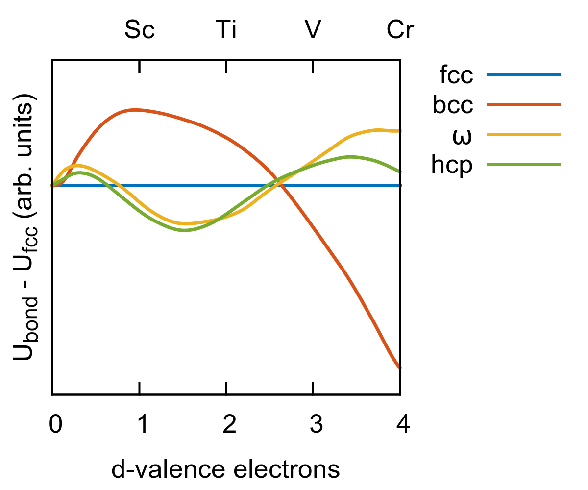 Figure 1
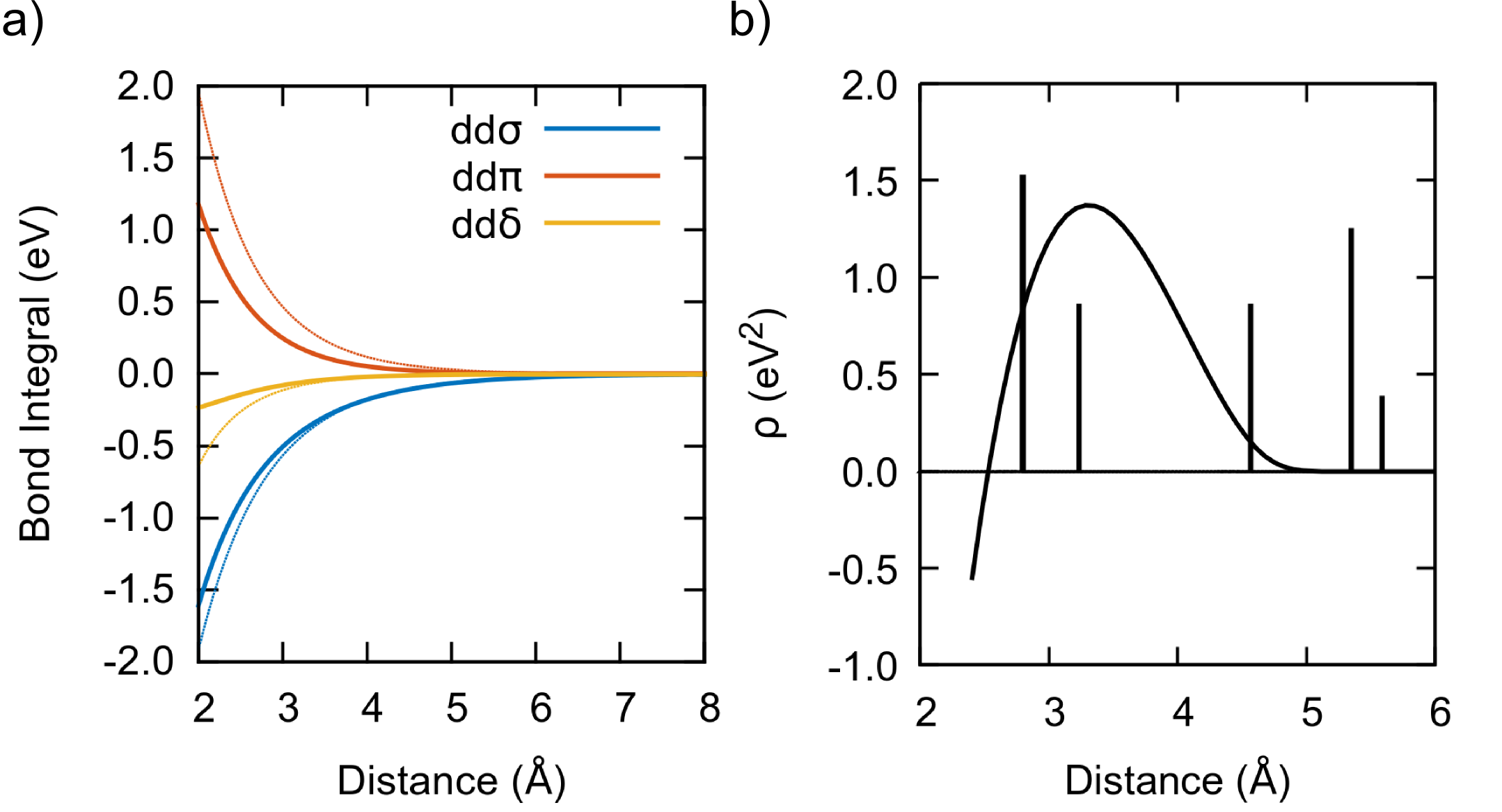 Figure 2
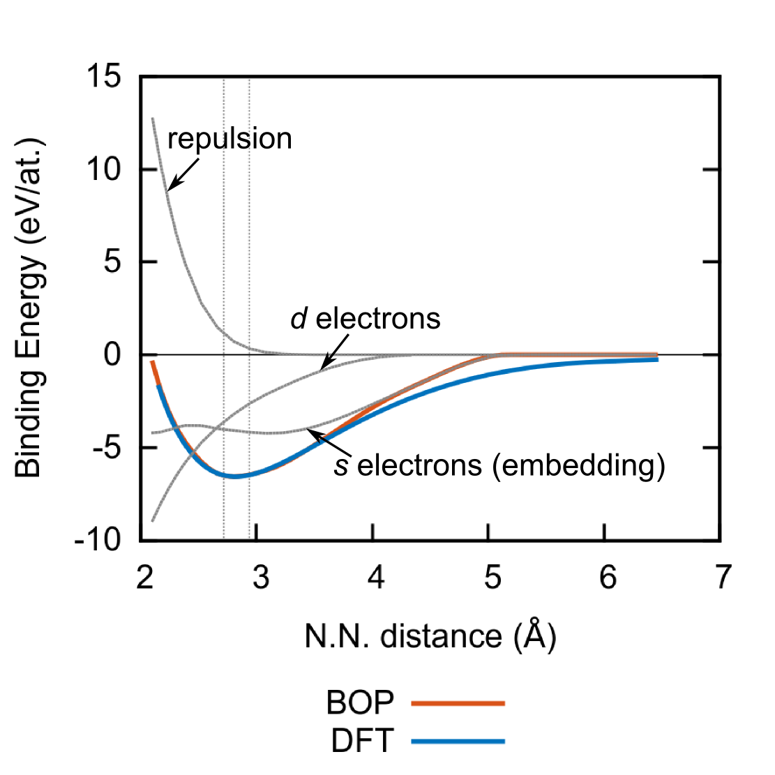 Figure 3
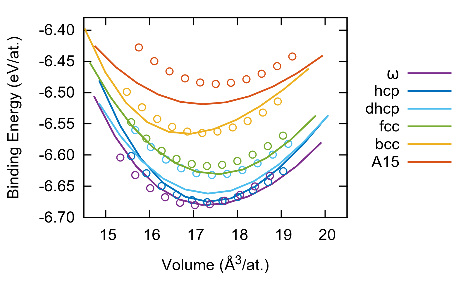 Figure 4
 Figure 5
 Figure 6
 Figure 7
 Figure 8
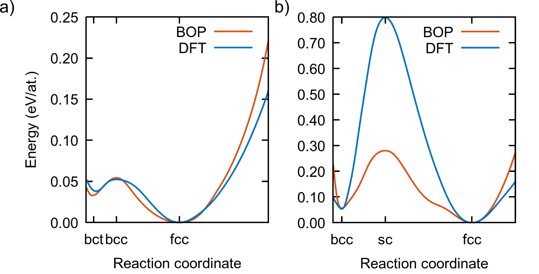 Figure 9
| exp. | DFT (this work) | NOTB (Trinkle et al.Trinkle et al. (2006)) | BOP (Girshick et al. Girshick et al. (1998a)) | BOP (this work) | |
|---|---|---|---|---|---|
| 4.626 Akahama et al. (2001) | 4.563 | 4.580 | 4.520 | 4.575 | |
| 0.608 Akahama et al. (2001) | 0.620 | 0.619 | 0.639 | 0.622 | |
| 112 Tane et al. (2013) | 112 | – | 81 | 106 | |
| 179 Tane et al. (2013) | 193 | 184 | 146 | 151 | |
| 90 Tane et al. (2013) | 79 | 90 | 79 | 89 | |
| 61 Tane et al. (2013) | 52 | 52 | 40 | 60 | |
| 228 Tane et al. (2013) | 241 | 261 | 118 | 234 | |
| 71 Tane et al. (2013) | 56 | 100 | 12 | 28 | |
| hcp | |||||
| 2.950 Fisher and Renken (1964) | 2.928 | 2.940 | 2.954 | 2.922 | |
| 1.587 Fisher and Renken (1964) | 1.586 | 1.602 | 1.587 | 1.604 | |
| 110 Fisher and Renken (1964) | 123 | – | 114 | 117 | |
| 176 Fisher and Renken (1964) | 196 | 155 | 176 | 170 | |
| 87 Fisher and Renken (1964) | 71 | 91 | 75 | 96 | |
| 68 Fisher and Renken (1964) | 83 | 79 | 84 | 86 | |
| 191 Fisher and Renken (1964) | 191 | 173 | 184 | 144 | |
| 51 Fisher and Renken (1964) | 39 | 65 | 51 | 29 | |
| bcc | |||||
| 3.310 Petry et al. (1991) | 3.263 | 3.27 | 3.231 | 3.228 | |
| 88 Ledbetter et al. (2004), 118 Petry et al. (1991) | 105 | – | 108 | 113 | |
| 98 Ledbetter et al. (2004), 134 Petry et al. (1991) | 104 | 87 | 95 | 83 | |
| 83 Ledbetter et al. (2004), 110 Petry et al. (1991) | 116 | 112 | 115 | 129 | |
| 38 Ledbetter et al. (2004), 36 Petry et al. (1991) | 36 | 31 | 58 | 37 |
| Prototype | - | Prototype | - | ||||
|---|---|---|---|---|---|---|---|
| C32 () | 6.680 | 6.680 | 0.000 | A17 (black P) | 6.517 | 6.563 | 0.046 |
| A3 (hcp) | 6.676 | 6.676 | 0.000 | A (-U) | 6.507 | 6.514 | 0.007 |
| Korbmacher (2019) | 6.672 | 6.675 | 0.003 | A15 (Cr3Si) | 6.486 | 6.519 | 0.033 |
| C19 (-Sm) | 6.651 | 6.666 | 0.015 | A12 (-Mn) | 6.486 | 6.558 | 0.072 |
| A3’ (dhcp) | 6.632 | 6.662 | 0.030 | A11 (-Ga) | 6.454 | 6.190 | -0.264 |
| A1 (fcc) | 6.617 | 6.631 | 0.014 | C14 (MgZn2) | 6.426 | 6.392 | -0.034 |
| A14 (I2) | 6.599 | 6.516 | -0.083 | C15 (Cu2Mg) | 6.421 | 6.338 | -0.083 |
| A (-Np) | 6.579 | 6.587 | 0.008 | A5 (-Sn) | 6.243 | 6.541 | 0.298 |
| A2 (bcc) | 6.565 | 6.566 | 0.001 | A (sc) | 5.838 | 6.345 | 0.507 |
| A13 (-Mn) | 6.558 | 6.537 | -0.021 | A9 (graphite) | 5.681 | 5.405 | -0.276 |
| exp. | DFT (this work) | NOTB (Trinkle et al.Trinkle et al. (2006)) | BOP (Girshick et al. Girshick et al. (1998a)) | BOP (this work) | |
|---|---|---|---|---|---|
| hcp defects | |||||
| [eV] | De Boer et al. (1988) | 1.92-2.07 Raji et al. (2009) | 1.81 | 2.33 | 2.80 |
| [mJ/m2] | 2100 Köppers et al. (1997) | 1939 Hennig et al. (2008) | – | 1454 | 2083 |
| [mJ/m2] | 1920 Tyson and Miller (1977) | 2451 Hennig et al. (2008) | – | 1571 | 2337 |
| [mJ/m2] | – | 1875 Hennig et al. (2008) | – | 1741 | 2271 |
| [mJ/m2] | – | 149 Benoit et al. (2012) | – | 38 | 62 |
| [mJ/m2] | – | 259 Benoit et al. (2012) | – | 106 | 160 |
| [mJ/m2] | – | 353 Benoit et al. (2012) | – | 171 | 256 |
| defects | |||||
| [eV] | – | 2.92 Trinkle et al. (2006) | 2.85 | 2.78 | 3.34 |
| [eV] | – | 1.57 Trinkle et al. (2006) | 1.34 | 0.68 | 1.61 |
| [mJ/m2] | – | 2131 Hennig et al. (2008) | – | 1764 | 2527 |
| [mJ/m2] | – | 2179 Hennig et al. (2008) | – | 1776 | 2490 |
| [mJ/m2] | – | 2435 Hennig et al. (2008) | – | 1460 | 2099 |
Peer Reviews
No public reviews on file for this paper yet. If you reviewed it on a platform where reviews are public (OpenReview, ICLR, NeurIPS, ICML), you can paste yours below so the community can read it here.
Videos
No videos yet. Explain this paper in a talk, walkthrough, or lecture? Add one.
Phase transitions in titanium with an analytic bond-order potential
Alberto Ferrari
Interdisciplinary Centre for Advanced Materials Simulation, Ruhr-Universität Bochum, 44801 Bochum, Germany
Malte Schröder
Interdisciplinary Centre for Advanced Materials Simulation, Ruhr-Universität Bochum, 44801 Bochum, Germany
Yury Lysogorskiy
Interdisciplinary Centre for Advanced Materials Simulation, Ruhr-Universität Bochum, 44801 Bochum, Germany
Jutta Rogal
Interdisciplinary Centre for Advanced Materials Simulation, Ruhr-Universität Bochum, 44801 Bochum, Germany
Matous Mrovec
Interdisciplinary Centre for Advanced Materials Simulation, Ruhr-Universität Bochum, 44801 Bochum, Germany
Ralf Drautz
Interdisciplinary Centre for Advanced Materials Simulation, Ruhr-Universität Bochum, 44801 Bochum, Germany
Abstract
Titanium is the base material for a number of technologically important alloys for energy conversion and structural applications. Atomic-scale studies of Ti-based metals employing first-principles methods, such as density functional theory, are limited to ensembles of a few hundred atoms. To perform large-scale and/or finite temperature simulations, computationally more efficient interatomic potentials are required. In this work, we coarse grain the tight-binding (TB) approximation to the electronic structure and develop an analytic bond-order potential (BOP) for Ti by fitting to the energies and forces of elementary deformations of simple structures. The BOP predicts the structural properties of the stable and defective phases of Ti with a quality comparable to previous TB parametrizations at a much lower computational cost. The predictive power of the model is demonstrated for simulations of martensitic transformations.
I Introduction
Titanium alloys are very attractive materials for structural and functional applications, superior to steels concerning the stiffness-to-weight and strength-to-weight ratios, corrosion resistance, and biocompatibility Ashby and Jones (1998). Ti-based materials are also characterized by unique elastic and mechanical properties, such as the shape memory alloys Ti-Ni Buehler et al. (1963), Ti-Pd, Ti-Pt, Ti-Au Doonkersloot and Vucht (1970), Ti-Nb Kim et al. (2006), Ti-Ta Bagarjatskii et al. (1958); Ferrari et al. (2019) and Ti-Mo Endoh et al. (2017), or the gum metals Ti-Nb-Ta-Zr-O and Ti-Ta-Nb-V-Zr-O Saito et al. (2003).
The remarkable properties of Ti alloys descend from the rich phase diagram of this element: Ti has five thermodynamically stable solid phases, the phase (hcp, spacegroup , Strukturbericht designation A3), the phase (bcc, , A2), the phase (hexagonal, , C32), and the Vohra and Spencer (2001) and Akahama et al. (2001) phases (both orthorhombic, , A20). At room temperature and ambient pressure, Ti is hcp and transforms martensitically to bcc at high temperatures and to , , and at high pressures. At zero temperature and pressure, not accessible to experiments, there is a general consensus that the ground state is the phase Trinkle (2003), which is more stable than hcp, and by less than 10 meV/at. and bcc by more than 100 meV/at.
Atomistic investigations of fundamental structural and thermodynamic properties of Ti-based materials are commonly performed using density functional theory (DFT). However, DFT calculations are limited to small length- ( 5 nm3) and time- ( 10 ps) scales and therefore direct studies of extended defects or phase transitions are usually not possible. To carry out such simulations, several empirical potentials have been fitted to experimental or first-principles data. These potentials are generally classical potentials based on the embedded atom method (EAM) Daw and Baskes (1984) or modified embedded atom method (MEAM) Baskes (1992). Such empirical models are unable to fully capture subtle features of the mixed metallic-covalent bonding in Ti and this often leads to quantitative or even qualitative discrepancies in the predicted properties of some phases. For instance, it has been reported that an accurate description of the phase Ackland (1992); Zope and Mishin (2003); Zhou et al. (2004); Ko et al. (2015); Gibson et al. (2016); Dickel et al. (2018) or of the temperature-dependent behaviour of the bcc phase Mendelev et al. (2016); Kartamyshev et al. (2019) needs to be sacrificed to achieve an overall good accuracy of the potential. A few potentials have succeeded to reproduce at least the , , and phases quantitatively Hennig et al. (2008); Ehemann and Wilkins (2017); Takahashi et al. (2017) by increasing the model complexity and by employing non-smooth interpolators, which however might lead to overfitting. The transferability of these more complex potentials to properties or environments not included in the training has been questioned Gibson et al. (2016); Rawat and Mitra (2017).
An alternative to DFT and classical potentials are tight-binding (TB) models Slater and Koster (1954); Ashcroft and Mermin (1976); Mehl and Papaconstantopoulos (1996, 2002); Rudin et al. (2004); Trinkle (2003); Trinkle et al. (2006); Margine et al. (2011); Cawkwell et al. (2015). Nonorthogonal TB models with -basis have been proven successful in the description of the most relevant properties of the hcp, bcc, , and phases in Ti Mehl and Papaconstantopoulos (2002); Trinkle et al. (2006). These TB models contain more than 100 parameters and their parameterization is often elaborate. In addition, similiarly to DFT, the diagonalization of the Hamiltonian and overlap matrices results in an unfavorable cubic scaling of the computational cost with the number of atoms. Hence, there is a demand for models that capture the essential characteristics of the electronic structure of Ti but are computationally efficient and simple to construct. One of such schemes are bond-order potentials (BOPs) Pettifor (1989); Horsfield et al. (1996); Pettifor et al. (2002); Drautz and Pettifor (2006), linear scaling interatomic potentials derived by coarse graining the TB method. Unfortunately, the only BOP for Ti in the literature Girshick et al. (1998a, b) fails to accurately reproduce crucial properties of this element, including the cohesive energies of the , fcc, and bcc phases, because its parametrization focused mainly on the hcp structure.
In this work, we develop a new, simple -valent analytic BOP for Ti and solve some of the critical flaws of the previous BOP for Ti. Our model contains only 25 adjustable parameters fitted to DFT energies of elementary structures at 0 K conditions. Despite its simplicity, our BOP accurately describes the main features of the bonding in Ti: it shows a good transferability to atomic environments not included in the fit set, qualitative agreement with first principles calculations on high-pressure and defective structures, and quantitative agreement with experiments regarding finite temperature properties.
This article is organized as follows: Sec. II introduces the theoretical background, the level of approximation and the structure of our model for Ti. Sec. III describes the fitting strategy with the database of fitted quantities and basic validation tests. Sec. IV contains the data on simple structures at 0 K. Sec. V studies the defect properties. Sec. VI presents the tests of the potential on the phase transitions induced by temperature and pressure before we conclude our work in Sec. VII.
II Methodology
Ti has four valence electrons; formally, two of these electrons have an -character and the remaining two a -character. To maximize the completeness of the TB representation, TB models for Ti usually employ a full nonorthogonal basis set that contains , , and angular components (a nonorthogonal spd model). This means that ten bond and ten overlap integrals (, , , , , , , , , in the Slater-Koster notation Slater and Koster (1954)) have to be parametrized as a function of the interatomic distance, making the fitting procedure of these models rather cumbersome.
Nonorthogonal models can be simplified in three conceptual steps. In a first step, at the cost of introducing an environmental dependence of the bond integrals Nguyen-Manh et al. (2000), the number of fitting parmeters can be halved by considering an orthogonal TB model, which can be derived from a nonorthogonal one by applying, for instance, Löwdin symmetric orthogonalization Löwdin (1950); Urban et al. (2011):
[TABLE]
where and are the Hamiltonian matrices of orthogonal and nonorthogonal models, respectively, and is the overlap matrix in the nonorthogonal model. In a second step, the explicit treatment of interactions between orbitals with - and -characters can be neglected, since the unsaturated directional bonds governing the structural stability of transition metals originate predominantly from the -electron interactions Pettifor (1970). As described in detail below, an orthogonal -only model is sufficient to correctly capture the small energy differences between the most stable phases of Ti. Finally, in a third step, the TB model can be coarse-grained to a BOP.
II.1 Significance of an orthogonal -only model
To prove that the relative stability of the thermodynamically stable phases of Ti can be captured by an orthogonal -only model, we employed the structural energy difference theorem Pettifor (1986); Seiser et al. (2011). At low pressure the orthorhombic phases and are degenerate with the hcp structure, hence we focused only on the hcp, bcc, and structures. The binding energy of a given atomic configuration is the sum of a bonding term , in this case due to the -electrons only, and a repulsive term :
[TABLE]
The structural energy difference theorem states that, to first order, the binding energy difference between two structures at equilibrium distance is
[TABLE]
that is, the relative stability can be evaluated by comparing the bonding terms of the two structures, provided that the repulsive contributions of the two structures are the same.
Here, for a qualitative description of , we chose an orthogonal -only model with the bond integrals having the canonical form Pettifor (1977); Andersen et al. (1978)
[TABLE]
where is the interatomic distance and is a constant that has the unit of energy. Only the contributions from the first nearest neighbor shells for fcc, and hcp, and the first two nearest neighbor shells for bcc were considered.
is given as a sum of a pairwise repulsion between the atoms
[TABLE]
For an approximate evaluation of the relative phase stability, may be assumed to be dominated by the overlap contribution and thus proportional to the square of the bond integrals Pettifor (1995); Seiser et al. (2011)
[TABLE]
Using this simplified model, we varied the volume per atom of bcc, hcp, and fcc phases to ensure their repulsive contributions were equal and compared for all four phases. Fig. 1 shows as a function of the -band filling (the number of electrons). For a band filling of roughly 2.0-2.3 electrons, corresponding to Ti, Zr, and Hf, the canonical bond integrals predict the correct ordering of the most important phases in Ti, with the phase slightly more stable than hcp, and bcc considerably higher in energy. This means that a simple orthogonal -only model does provide the correct phase stability in Ti.
II.2 Bond-order potentials
Given that the -valence electrons are sufficient to take into account the phase ordering in Ti, we aimed for a -only model to develop our interatomic potential. Instead of a TB model, we parametrized a more computationally efficient BOP. Besides the already mentioned potential for titanium Girshick et al. (1998a, b), -valent BOPs have been proven very successfull for many other transition metals, including molybdenum Mrovec et al. (2004); Čák et al. (2014); Lin et al. (2014), iridium Cawkwell et al. (2005, 2006), tungsten Mrovec et al. (2007); Čák et al. (2014); Lin et al. (2014), iron Mrovec et al. (2011); Lin et al. (2016), niobium, tantalum Čák et al. (2014); Lin et al. (2014), and manganese Drain et al. (2014).
BOPs are linear scaling quantum-mechanical potentials that retain information on the TB electronic structure via the moments of the local density of states (DOS). The -th moment of the DOS of the orbital on atom is
[TABLE]
The moments of the DOS are related to the crystal structure via the moments theoremCyrot-Lackmann (1967); Jenke et al. (2018), which links the -th moment to a self-returning hopping path of length starting and ending on the orbital , assuming an orthonormal basis,
[TABLE]
[TABLE]
If only the first moments are considered, the local DOS, total energy, and forces can be calculated analytically from the self-returning paths of lengths at a computational cost that scales linearly with the number of atoms in the simulation cell Pettifor (1989); Horsfield et al. (1996); Drautz and Pettifor (2006); Seiser et al. (2013). BOPs thus offer a great computational advantage over orthogonal TB models with only a minor sacrifice in accuracy related to the truncation of the moments expansion.
In this work we employed analytic BOPs Drautz and Pettifor (2006, 2011); Seiser et al. (2013). All BOP calculations were performed using the BOPfox code Hammerschmidt et al. (2019) with a value of and a terminator of 200 constant recursion coefficients.
II.3 The BOP model for Ti
The binding energy in our BOP model is expressed as
[TABLE]
The bonding energy depends on the , , and two-center bond integrals. We modeled the distance dependence of the bond integrals with the sum of two exponential functions:
[TABLE]
where , , and are adjustable parameters. The bond integrals were multiplied by a cutoff function,
[TABLE]
in the range to ensure their smooth decay to zero. Values of 4.45 Å and 1.35 Å were chosen for and , respectively.
Following Madsen et al. Madsen et al. (2011) and Drain* et al.* Drain et al. (2014), an embedding function was introduced to mimic the contribution of the missing electrons and hybridization to the cohesive energy. The embedding term was parameterized using a Finnis-Sinclair Finnis and Sinclair (1984) second-moment expression:
[TABLE]
where is represented by a smooth third-order spline function with only two nodes. Albeit empirical, the embedding term mimics the bonding contribution of electrons acting as a homogeneous gas of nearly-free electrons with density , in direct analogy to the EAM potentials.
Finally, the repulsive term , including the overlap, electrostatic, exchange-correlation, and double counting contributions, was parameterized using a pairwise expression (Equation (5)), where is an exponential function with three fitting parameters
[TABLE]
Motivated by the qualitative results obtained with the canonical model (Figure 1), we fixed the number of electrons in our BOP to 2.1. Changes in the number of electrons in the range 2.0-2.7 followed by refitting did not improve the quality of the interatomic potential.
III Fitting strategy
III.1 Fitting database
Our fitting database Lysogorskiy et al. (2019) consisted of high-quality DFT energies and forces for different atomic configurations calculated using the Vienna Ab initio Simulation Package (VASP 5.4) Kresse and Hafner (1993); Kresse and Furthmüller (1996a, b) following the pyiron workflow Janssen et al. (2019). For all DFT calculations we used a projector-augmented wave (PAW) pseudopotential Blöchl (1994); Kresse and Joubert (1999) with 12 valence electrons and the exchange-correlation potential with the generalized-gradient expression by Perdew, Burke, and Ernzerhof (PBE) Perdew et al. (1996). Standard values of 500 eV and 0.1 Å were employed for the energy cutoff and -point linear density, respectively, to minimize the numerical errors. The -points were distributed in the Brillouin zone with the Monkhorst-Pack Baldereschi (1973); Monkhorst and Pack (1976) special -point technique. The electronic occupations were smeared using the Methfessel-Paxton function of order one Methfessel and Paxton (1989) with a width of 0.2 eV.
The ground state energies of the , hcp, double-hcp (dhcp), fcc, bcc, and A15 structures were carefully determined by optimizing the volume and the ratio in the hexagonal structures to ensure a precision of the obtained energies within less than 1 meV/at. Typically, the optimizations were done in two or three stages to minimize the Pulay stresses Dacosta et al. (1986).
Furthermore, the equilibrium cell of each phase was deformed isotropically within a volume range to obtain energy-volume curves. For the , hcp, and bcc phases we evaluated also the elastic constants, by considering a series of symmetrically inequivalent deformations (0.5%) Golesorkhtabar et al. (2013); Lysogorskiy et al. (2019), and the phonon spectra, using the small displacements method as implemented in Phonopy Togo and Tanaka (2015).
The BOP binding energy per atom is related to the DFT energy per atom of the pseudopotential calculation by
[TABLE]
where is the total energy of isolated Ti atoms. Since our BOP model is constructed with respect to a non-magnetic Ti atom with electronic configuration , we took as the energy of a spin-unpolarized Ti atom with the same electronic configuration. For the pseudopotential used in this work, we obtained eV.
III.2 Fitting procedure
We optimized our interatomic potential using the Levenberg-Marquardt Levenberg (1944); Marquardt (1963) least-squares method as implemented in the Bond-Order Potential Characterization, Assessment, and Testing (BOPcat) suite Ladines (2019). The starting parameters for the bond integrals were taken from a projection of the DFT wavefunction on an orthogonal TB basis set for the Ti dimer. The details of the projection method can be found in Ref. Jenke, 2019. In a first step, we considered a full model derived from the Ti dimer and fitted the parameters , , and in the repulsive term to reproduce the DFT binding energy-volume curves of the , hcp, fcc, bcc, and A15 structures as closely as possible. We then substituted the explicit treatment of the electrons with the embedding function and determined the four parameters of this function to reproduce the same DFT data, keeping the bond integrals and the repulsive term fixed. Finally, for the , hcp, and bcc structures only, we added to the fitting database the binding energies of the elastically deformed structures and the forces resulting from the small displacements method for the phonons. At this stage, the energy-volume curve of the dhcp phase was also included. In the final optimization step, all 25 model parameters were adjusted. The optimized values of the parameters for our model are listed in Tab. 1 of the Supplemental Material Sup .
Fig. 2a displays the distance dependence of the , , and bond integrals as derived from the Ti dimer projections (thin lines) and after full optimization (thick lines). As expected, the range of the bond integrals becomes shorter after optimization because in the bulk environment the interactions are screened by the charge densities of neighboring atoms Nguyen-Manh et al. (2000). It is worth noting that at a distance of 2.9 Å, corresponding approximately to the first nearest neighbor shell for most structures, the ratio of the optimized bond integrals is , that is close to the canonical ratio employed in Sec. II.1.
Fig. 2b shows the optimized embedding function , superimposed on the radial distribution function of bcc at the equilibrium volume. has a maximum at approximately 3.3 Å, roughly at the second nearest-neighbor, and decreases smoothly to zero for long interatomic distances. This variation is consistent with our analysis of and TB models obtained by a projection of pseudo-atomic orbitals on DFT wave functions Urban et al. (2011) and will be discussed in detail elsewhere Mrovec (2019). At extremely short distances ( 2.5 Å), outside the fitting range, becomes negative. This is interpreted as a many-body repulsive overlap contribution due to overlapping charge densities.
The contributions of the bonding, embedding, and repulsive terms for our BOP for bcc Ti are marked by grey lines in Fig. 3. The electrons contribute approximately 40% to the cohesive energy, while the remaining part is due to the electrons. This agrees with the respective contributions to the cohesive energy derived from and orbital projections Urban et al. (2011).
The (total) binding energy calculated with our potential (red line in Fig. 3) agrees very well with the DFT binding energy (blue line in Fig. 3) even for interatomic distances well outside the fitting range (delineated by the dashed vertical lines in Fig. 3). This denotes an outstanding transferability of our BOP to structures with both small and large densities. The BOP binding energy starts deviating significantly from the DFT reference only at large interatomic distances exceeding 4 Å, where the embedding function decreases to zero.
IV Properties of bulk phases
The BOP (lines) and DFT (circles) binding energy-volume curves are compared for the fitted structures in Fig. 4. The cohesive energies of , hcp, and bcc are very well captured by our potential, while the energies of the fcc and A15 phases are slightly underestimated. The model also underestimates the energy of the double-hcp (dhcp) phase, which is important for the properties of basal stacking faults (see Sec. V). In Tab. 1 the equilibrium lattice parameters, bulk moduli, and elastic constants of the , hcp, and bcc phases as predicted by our potential are compared to our DFT results, the values computed with the BOP of Girshick et al. Girshick et al. (1998a), the results of a non-orthogonal TB model of Trinkle et al. Trinkle et al. (2006), and to available experimental values. For the and hcp structures, the DFT lattice parameters are very well reproduced by the BOP, while for bcc the lattice parameter is underestimated by 1% with respect to DFT. This is reflected in an underestimation of the volume of the bcc structure visible in Fig. 4. The quality of the bulk moduli and elastic constants is almost as good as that of the non-orthogonal TB model Trinkle et al. (2006), and the deviation from the experimental measurements is only about twice as large as the deviation between DFT and experiments. The present BOP describes the phase much better than the BOP by Girshick et al., who did not consider this phase in their parametrization, without compromising significantly the properties of the hcp and bcc structures. It is also worth pointing out that the elastic constants were not included directly in the fitting procedure of our potential, but they are related to the curvature of the energy-deformation curves in our training database.
Fig. 5 presents the phonon dispersion relations and densities of modes of the , hcp, and bcc phases for our BOP, DFT, and, where available, experiments. The acoustic phonons of the phase are slightly underestimated with respect to DFT, while the optical phonons are overestimated for all high-symmetry points except for the A zone boundary. The underestimation of the acoustic branches is a consequence of the underestimation of the elastic constant. These differences are also reflected in the phonon density of modes. The spectrum of hcp matches DFT and experiments quite closely, apart from softenings at the K and A points and the negative curvature of the optical branch at , which is a feature common to most interatomic potentials for hcp metals. The bcc phonons are also captured very well by our BOP, and the 0 K - and -instabilities at and , respectively, are both present.
To check the performance of our interatomic potential in different atomic environments, we computed the cohesive energy of some low-energy (up to 1 eV higher than the ground state) prototype structures using both DFT and BOP. The results for the various prototypes, indicated by their Strukturbericht designations and names of the most common compounds with that particular structure, are reported in Tab. 2. The structures included in the fit set are shown in bold. As deduced by the relatively small differences between the BOP predictions and the first principles data, the potential shows a remarkable transferability to very different coordination polyhedra and even to exotic structures, rarely considered during testing of interatomic potentials. The most significant differences between the cohesive energies of DFT and BOP are the simple cubic (sc), the A11 (-Ga), and A5 (-Sn) structures, all characterized by a relatively low cohesive energy. The average error for the considered prototypes is 90 meV/at.
To further test the BOP, we calculated the energy along the hexagonal and bcc transformation paths with DFT and with the present BOP, since these paths are crucial for the phase transitions in Ti. The details of the hexagonal transformation path can be found in Refs. Paidar et al., 1999; Luo et al., 2002; Čák et al., 2014; the bcc transition consists of a shuffling of pairs of atoms along the [111] direction of bcc, corresponding to the phonon Ehemann and Wilkins (2017). For simplicity, the volume of the unit cell was taken as constant along the transformations. The results, displayed in Fig. 6, show that both paths are very well reproduced by our BOP, even if the intermediate points were not included during the fitting.
V Defect properties
The properties of defects were completely absent from the fit set and therefore constitute an important test for the predictive capabilities of the developed potential for highly distorted atomic configurations around fundamental defects. We computed the formation energies of vacancies, low-index surfaces and fundamental stacking faults in the hcp and phases. The obtained results are listed in Tab. 3 together with the results from other TB models, the previous BOP, DFT, and experiments (where available).
The vacancy formation energies in both hcp and phases are overestimated by our BOP, but the relative stability of vacancies in the phase (which has two inequivalent Wyckoff positions and thus two different sites for the vacancy) is well reproduced. The values of the surface formation energies agree very well with the DFT values, in contrast to other classical potentials Ackland (1992); Zhou et al. (2004); Hennig et al. (2008); Gibson et al. (2016) and the previous BOP Girshick et al. (1998a, b), although the relative ordering of the energetics does not correspond to DFT. A relatively large systematic underestimation is obtained for the energies of the fundamental stacking faults on the basal plane of hcp. All three calculated stacking faults are about 100 mJ/m2 lower than the reference DFT values. This deviation is most likely related to underestimation of the dhcp energy by our model. According to DFT, the dhcp structure is 44 meV/at. less stable than hcp, whereas our BOP predicts only 14 meV/at. This discrepancy leads to the underestimation of stacking fault energies. An even more severe underestimation of the stacking fault energies is observed in the BOP by Girshick et al., pointing out that the correct description of the energy difference between hcp and dhcp and thus of the stacking faults might be beyond the limitations of -only models. Even with the explicit inclusion of dhcp in the fitting database, the cohesive energy of this structure could not be improved without compromising the stability of the other phases.
VI Thermodynamic properties
VI.1 Temperature-induced phase transformations
Ti exhibits a complex phase diagram that is challenging to reproduce using empirical interatomic potentials. We employed our BOP in molecular dynamics (MD) simulations at finite temperatures and focused on the phase transformations hcp, hcpbcc, and bccliquid at zero pressure. To estimate the transition temperatures for the two martensitic transformations hcp and hcpbcc we computed the free energies of the , hcp, and bcc phases. For and hcp, since these phases are dynamically stable at 0 K, we employed the harmonically assisted temperature integration method detailed in Ref. Moustafa et al., 2017. The free energy can then be decomposed as the sum of a harmonic term, which depends on the phonon density of modes at a given volume , and an anharmonic contribution ,
[TABLE]
[TABLE]
Following Ref. Moustafa et al., 2017, we computed as
[TABLE]
where , , and are respectively the potential energy, forces and displacements from the equilibrium positions extracted from MD simulations at various temperatures and volumes, and is the energy of the equilibrium or hcp phases. The thermal averages in Eq. (16) were calculated from MD trajectories in the ensemble with a duration of 10 ps after complete equilibration with a Langevin thermostat for 5 different volumes. For the phase we employed a supercell while for the hcp phase a supercell, with a total of 288 atoms for both structures. For each temperature, the obtained free energy-volume curves were fitted using the Birch-Murnaghan equation Murnaghan (1944); Birch (1947) to determine the value of the zero-pressure (Helmholtz) free energy.
Since the bcc structure is not stable at 0 K, temperature integration as in Eq. (16) is not possible. To calculate the free energy of the bcc phase, we instead employed the standard Frenkel-Ladd method Frenkel and Ladd (1984) to integrate the free energy difference between our potential and a reference potential ,
[TABLE]
choosing as the reference system an Einstein crystal with potential energy
[TABLE]
with eV/Å2. The thermal averages were again calculated in the ensemble for 10 ps using a bcc cubic supercell with 432 atoms. The volume was varied for each temperature so that the total pressure was zero. The integral in Eq. (17) was evaluated using 15 values of the switching parameter .
Fig. 7 presents the Helmholtz free energy differences between and hcp and between bcc and hcp as a function of temperature. The energy difference between and hcp at 0 K reduces to 3 meV/at. if the zero point energy is considered. Our BOP predicts a phase transition between and hcp at 205 K, in good agreement with non-orthogonal tight-binding (280 K) Rudin et al. (2004). This transition has never been measured experimentally at zero pressure because of the large free energy barrier that separates the two phases; however, the transformation temperature must be below room temperature, as correctly predicted by our BOP. The phase transition between hcp and bcc occurs for our potential at 1180 K, in excellent agreement with experiments that detect the transition at 1155 K Holland (1963).
Finally, we also estimated the melting point of Ti with our interatomic potential by gradually heating the bcc phase until melting was observed. For this calculation a bcc supercell in a slab geometry with two free surfaces was employed. The free surfaces in the periodic cells were separated in direction by roughly 5 nm of vacuum. The dimensions along the [010] and [001] directions were adjusted for each temperature to minimize the stresses. By analyzing the radial distribution function of the slab, we estimated a melting temperature of K, in good agreement with the experimental melting point (1941 K).
In general, the predictions of our BOP model for finite temperature thermodynamic properties show an impressive agreement with experiments even though the fitting database was composed only of 0 K data. This is perhaps the best exemplification of the excellent transferability of our potential to properties not included in the training set.
VI.2 Pressure-induced phase transformations
We also analyzed the predictions of our potential at non-zero pressure by varying the volume of the unit cell of the , hcp, and phases. At each volume, we optimized the ratio of the and hcp phases, and the and ratios and the atomic positions of the phase. The obtained energy-volume data were then fitted using the Birch-Murnaghan equation of state Murnaghan (1944); Birch (1947). The pressure and the enthalpy were evaluated according to
[TABLE]
Fig. 8 illustrates the enthalpy difference between hcp and and between and as a function of pressure. At negative pressure (expanded volume), the hcp phase becomes more stable than at -3 GPa, which agrees well with the DFT value of -5 GPa Hennig et al. (2008). At high pressures, the phase is stabilized, but the transition pressure of 23 GPa predicted by BOP is too low compared to experimental data ( GPa Vohra and Spencer (2001); Akahama et al. (2001)). This is, however, not unexpected as this phase transformation is known to be due to an - transition Vohra and Spencer (2001): at high pressure, the long-ranged orbitals become unfavourable and a fraction of -electrons is promoted to orbitals. This in turn increases the -band filling and stabilizes orthorhombic structures with respect to hexagonal ones. The form of our embedding function, which mimics the contribution from the electrons, is clearly too simple to quantitatively capture this mechanism. Nevertheless, the BOP model can reproduce qualitatively the correct sequence hcp with increasing pressure.
VII Conclusions
We developed a bond-order potential for Ti that retains the essential features of the electronic structure of this element without sacrificing the computational efficiency, thanks to the linear scaling analytical expressions for the energy and forces. The small number of parameters in our model did not preclude an accuracy comparable to more complex parametrizations regarding the structural properties of the , hcp, and bcc phases. On the contrary, the choice of a very simple, physically motivated model lead to an extraordinary transferability to various atomic configurations not considered in the fitting procedure, including diverse structures and prototypes not tested before. This transferability is also reflected in a good reproducibility of the energetics of some extended defects, and very accurate thermodynamic properties. The limitations of this potential include the mechanisms that involve critically the -electrons, such as the pressure-induced transition, and the stacking fault energies. Nevertheless, within its clearly delineated range of applicability, we believe that our potential is suitable not only for the atomistic characterization of the stable phases of Ti but also to explore new mechanisms in this intriguing material.
Acknowledgements.
A.F., J.R. and R.D. acknowledge financial support from the Deutsche Forschungsgemeinschaft (DFG) within the research unit FOR 1766 (High Temperature Shape Memory Alloys, http://www.for1766.de, project number 200999873, sub-group TP3), and Y.L. and R.D. through projects 405621217 and 405602047. M.S. acknowledges funding from the International Max Planck Research School (IMPRS) SurMat. Part of the calculations presented in this work were performed on the Tetralith and Sigma clusters of the Swedish National Infrastructure for Computing (SNIC) at the National Supercomputer Centre (NSC) in Linköping, and on the Beskow cluster at the Center for High Performance Computing (PDC) in Stockholm. The authors are grateful to Thomas Hammerschmidt and Alvin Ladines for the support with the BOPfox and BOPcat programs, respectively. A.F. thanks Tony Paxton for helpful suggestions on the fitting strategy and Sergej Starikov for fruitful discussions on the free energy of bcc Ti and the melting point.
The reference list from the paper itself. Each links out to its DOI / PubMed record.
- 1Ashby and Jones (1998) M. F. Ashby and D. R. H. Jones, Engineering Materials 2 (Elsevier, Oxford, 1998).
- 2Buehler et al. (1963) W. J. Buehler, J. V. Gilfrich, and R. C. Wiley, J. Appl. Phys. 34 , 1475 (1963).
- 3Doonkersloot and Vucht (1970) H. C. Doonkersloot and V. Vucht, J Less Common Met. 20 , 83 (1970).
- 4Kim et al. (2006) H. Y. Kim, Y. Ikehara, J. I. Kim, H. Hosoda, and S. Miyazaki, Acta Mater. 54 , 2419 (2006).
- 5Bagarjatskii et al. (1958) Y. A. Bagarjatskii, G. I. Nosova, and T. V. Tagunova, Dokl. Akad. Nauk SSSR 122 , 593 (1958).
- 6Ferrari et al. (2019) A. Ferrari, D. G. Sangiovanni, J. Rogal, and R. Drautz, Phys. Rev. B 99 , 094107 (2019).
- 7Endoh et al. (2017) K. Endoh, M. Tahara, T. Inamura, and H. Hosoda, J. Alloys Compd. 695 , 76 (2017).
- 8Saito et al. (2003) T. Saito, T. Furuta, J.-H. Hwang, S. Kuramoto, K. Nishino, N. Suzuki, R. Chen, A. Yamada, K. Ito, Y. Seno, et al., Science 300 , 464 (2003).