Statistical detection of a tidal stream associated with the globular cluster M68 using Gaia data
C. G. Palau, J. Miralda-Escud\'e

TL;DR
This paper introduces a maximum likelihood method to detect and analyze tidal streams in Gaia data, successfully identifying the M68 stream and providing insights into the Milky Way's gravitational potential.
Contribution
The paper presents a novel statistical method for detecting tidal streams and applies it to Gaia data, identifying the M68 stream and estimating the Milky Way's dark halo shape.
Findings
Detected the M68 tidal stream passing within 5 kpc of the Sun.
Confirmed the stream's association with the Fjörm stream.
Provided a list of 115 probable stream members for follow-up studies.
Abstract
A method to search for tidal streams and to fit their orbits based on maximum likelihood is presented and applied to the Gaia data. Tests of the method are performed showing how a simulated stream produced by tidal stripping of a star cluster is recovered when added to a simulation of the Gaia catalogue. The method can be applied to search for streams associated with known progenitors or to do blind searches in a general catalogue. As the first example, we apply the method to the globular cluster M68 and detect its clear tidal stream stretching over the whole North Galactic hemisphere, and passing within 5 kpc of the Sun. This is one of the closest tidal streams to us detected so far, and is highly promising to provide new constraints on the Milky Way gravitational potential, for which we present preliminary fits finding a slightly oblate dark halo consistent with other observations. We…
Click any figure to enlarge with its caption.
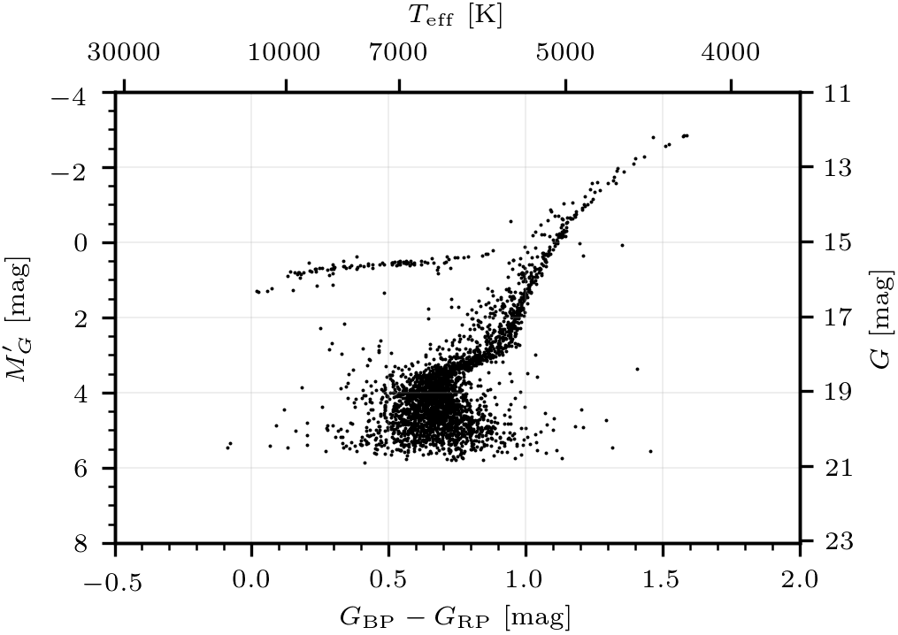 Figure 1
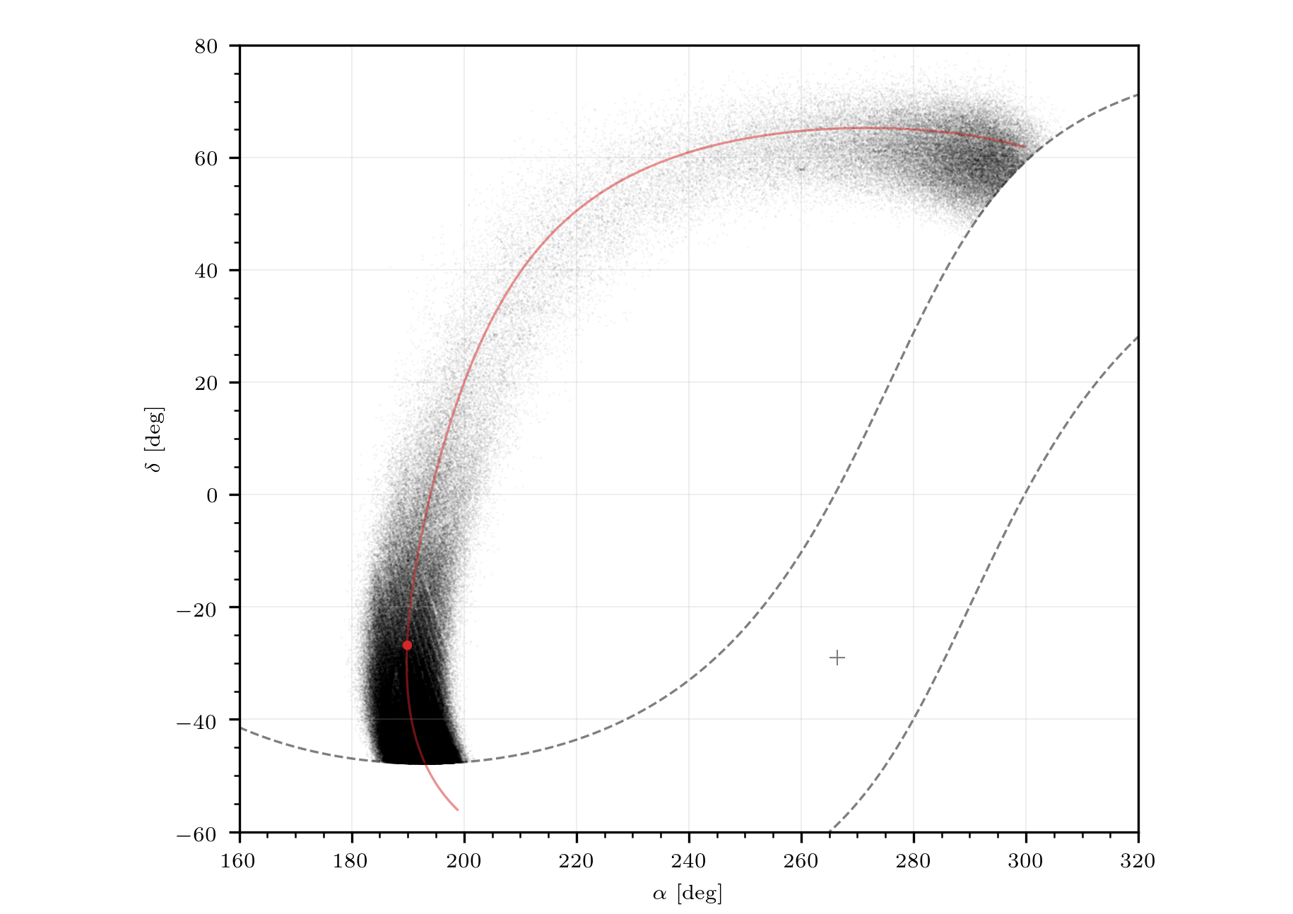 Figure 2
 Figure 3
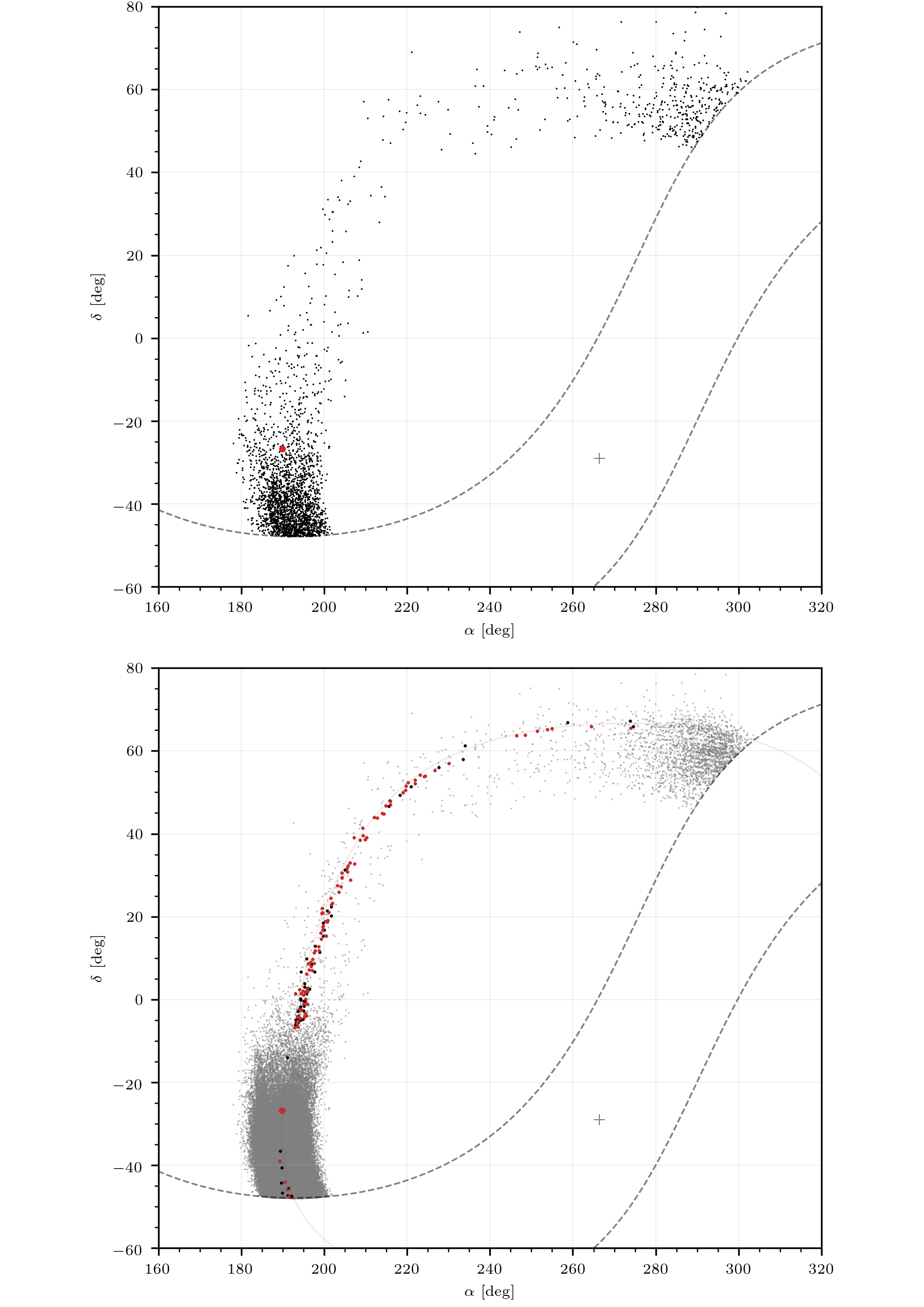 Figure 4
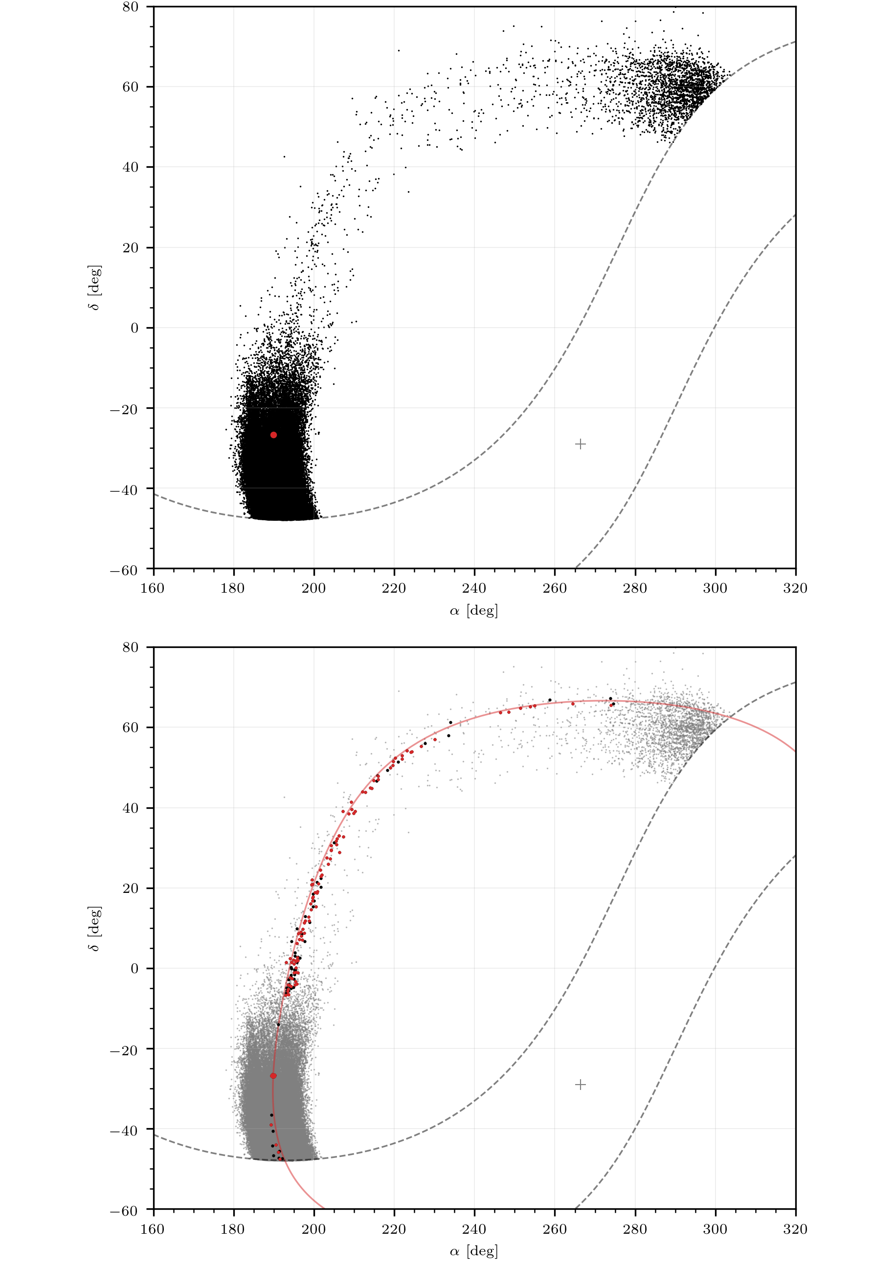 Figure 5
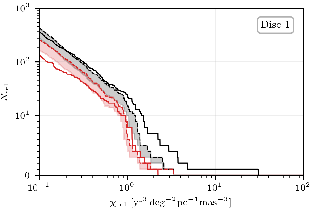 Figure 6
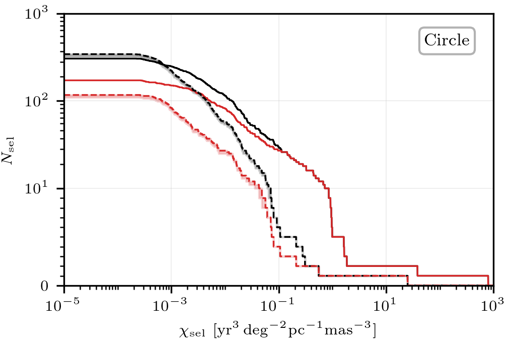 Figure 7
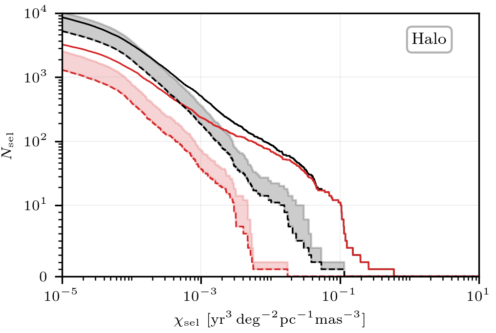 Figure 8
 Figure 9
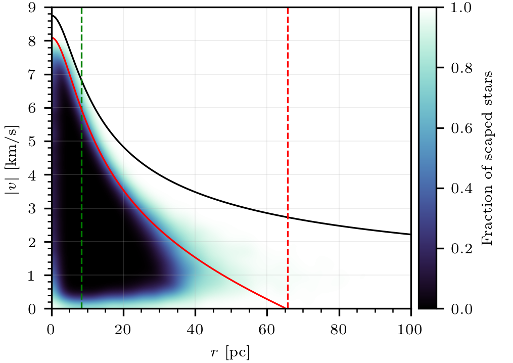 Figure 10
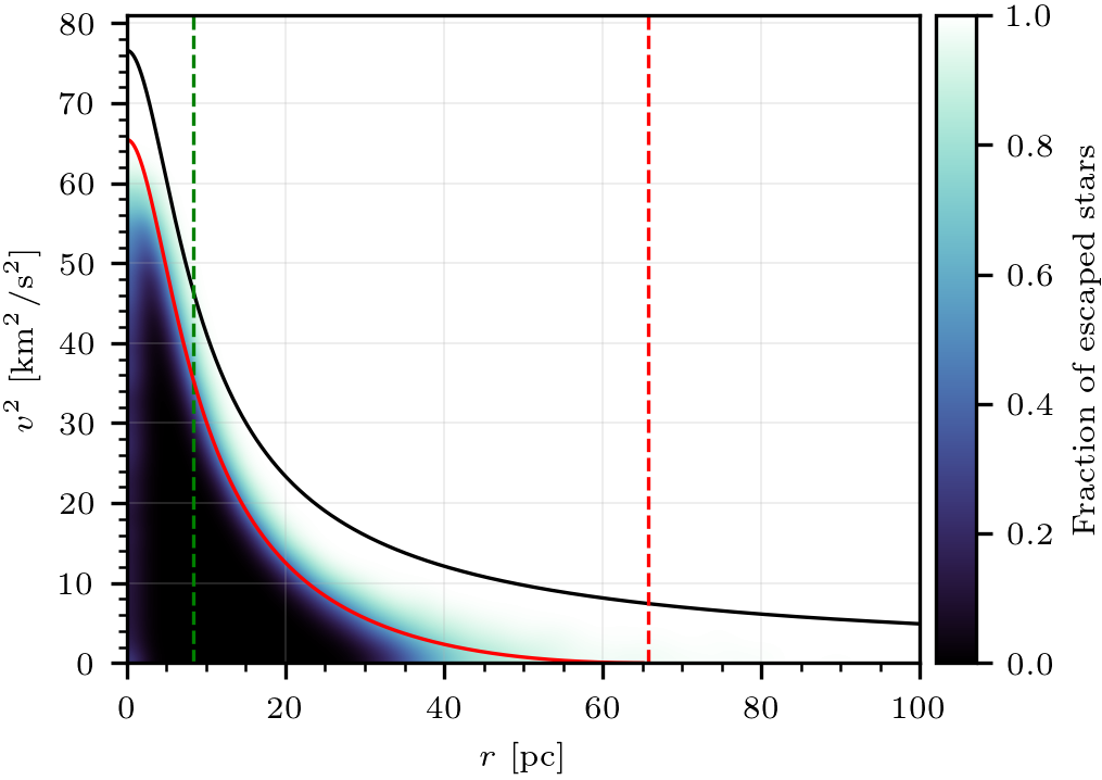 Figure 11
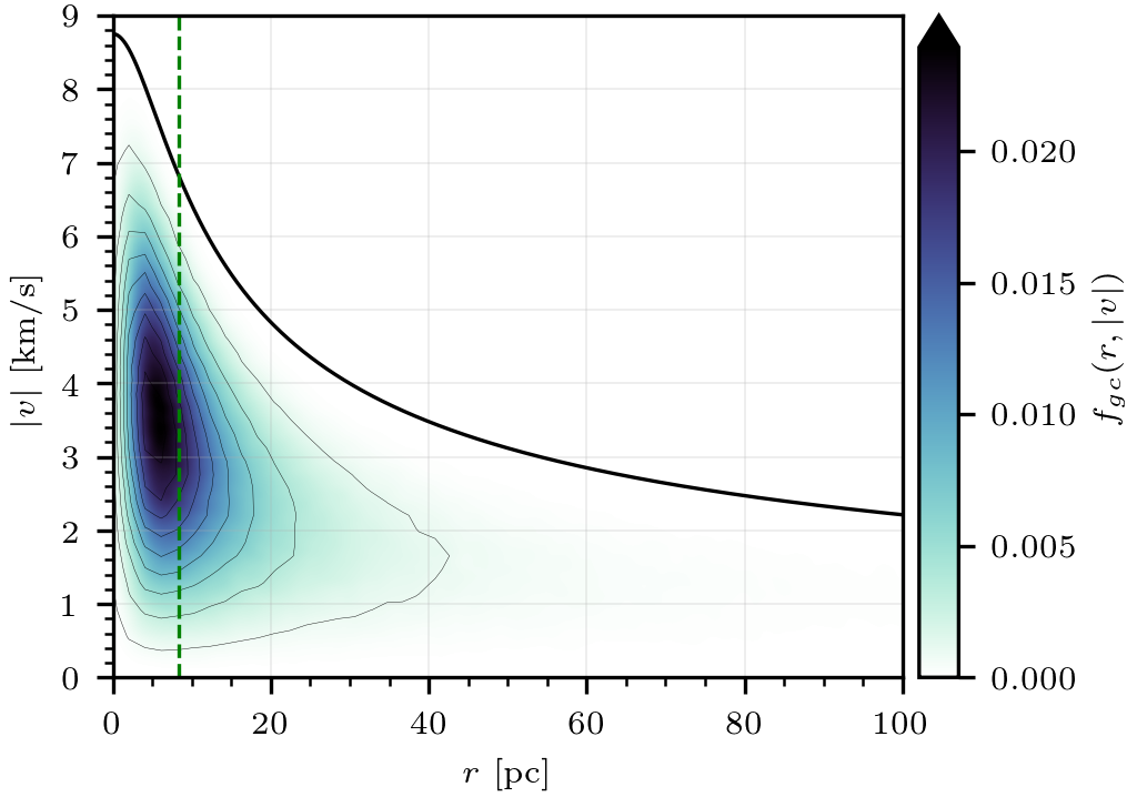 Figure 12
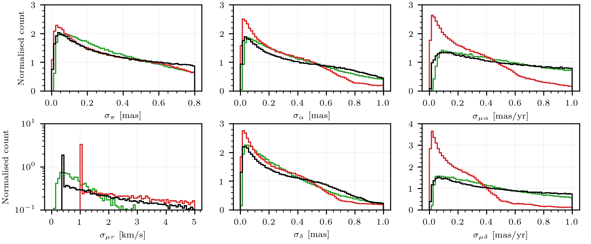 Figure 13
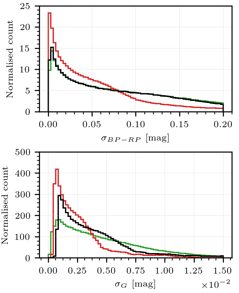 Figure 14
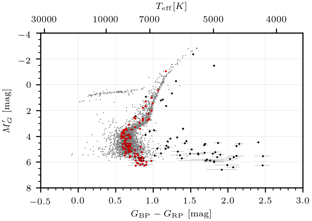 Figure 15
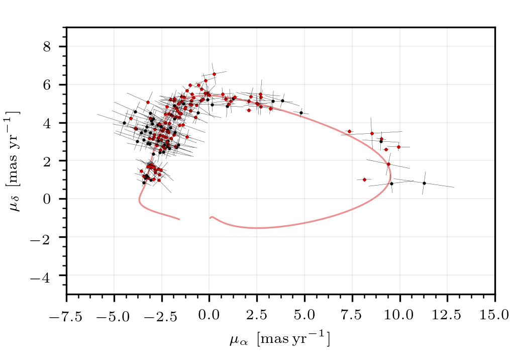 Figure 16
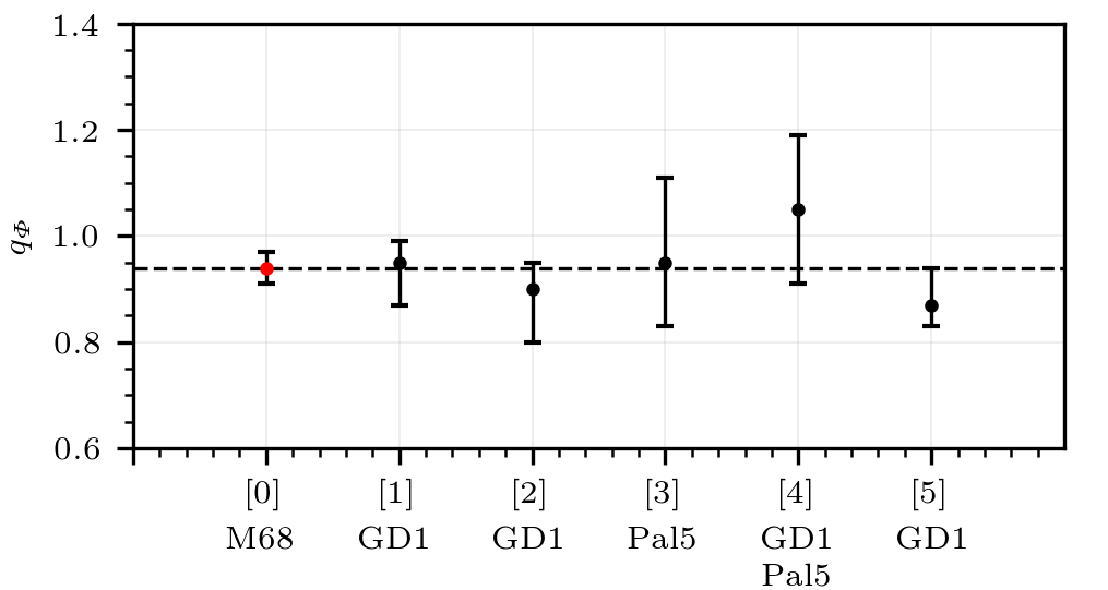 Figure 17
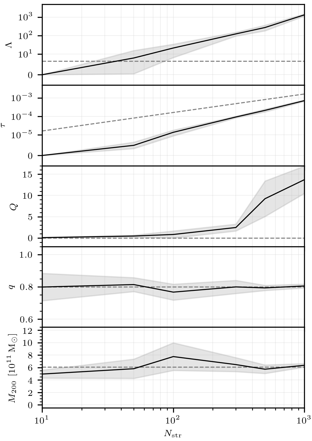 Figure 18
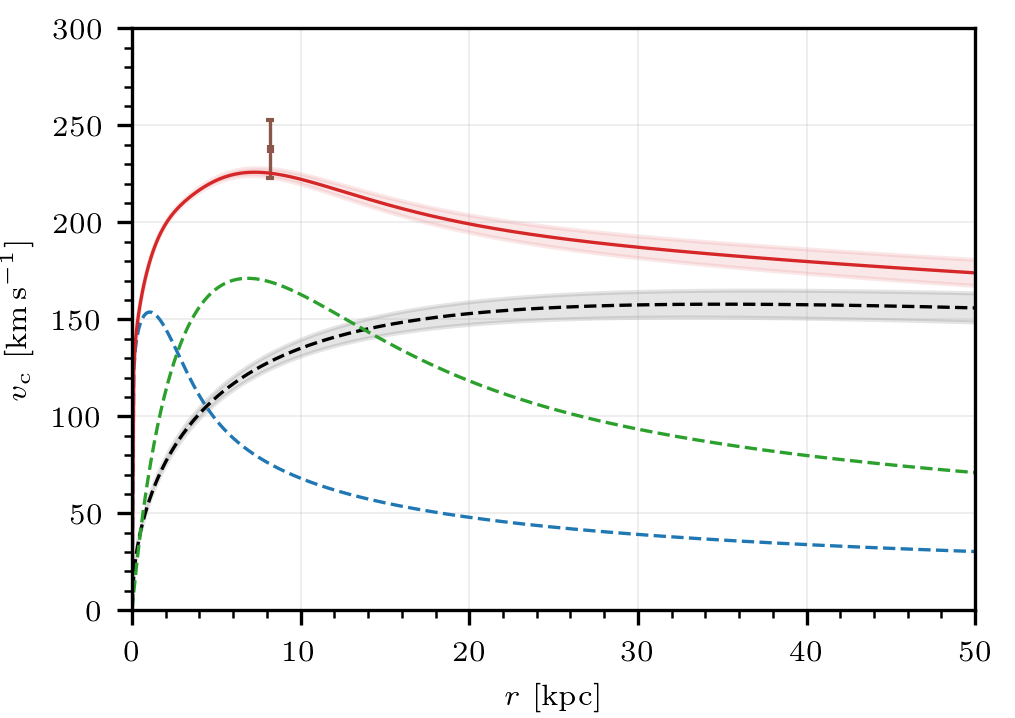 Figure 19
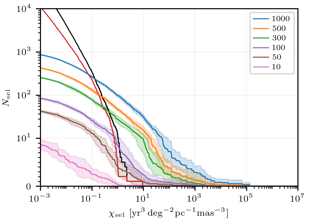 Figure 20
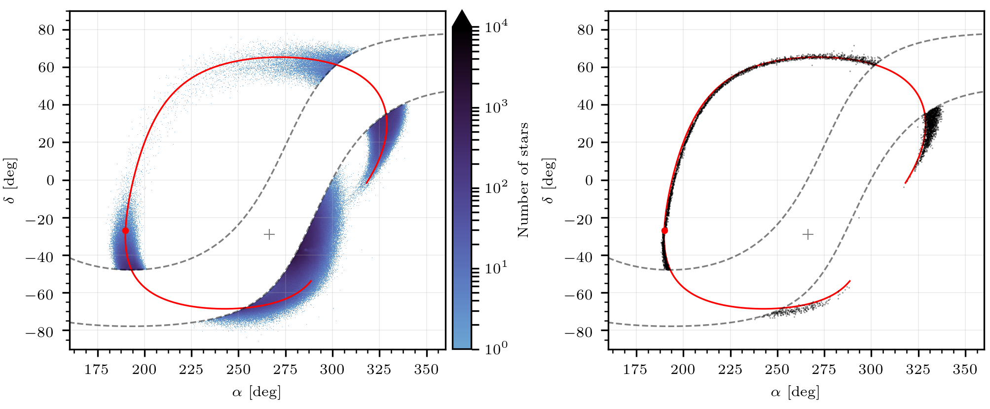 Figure 21
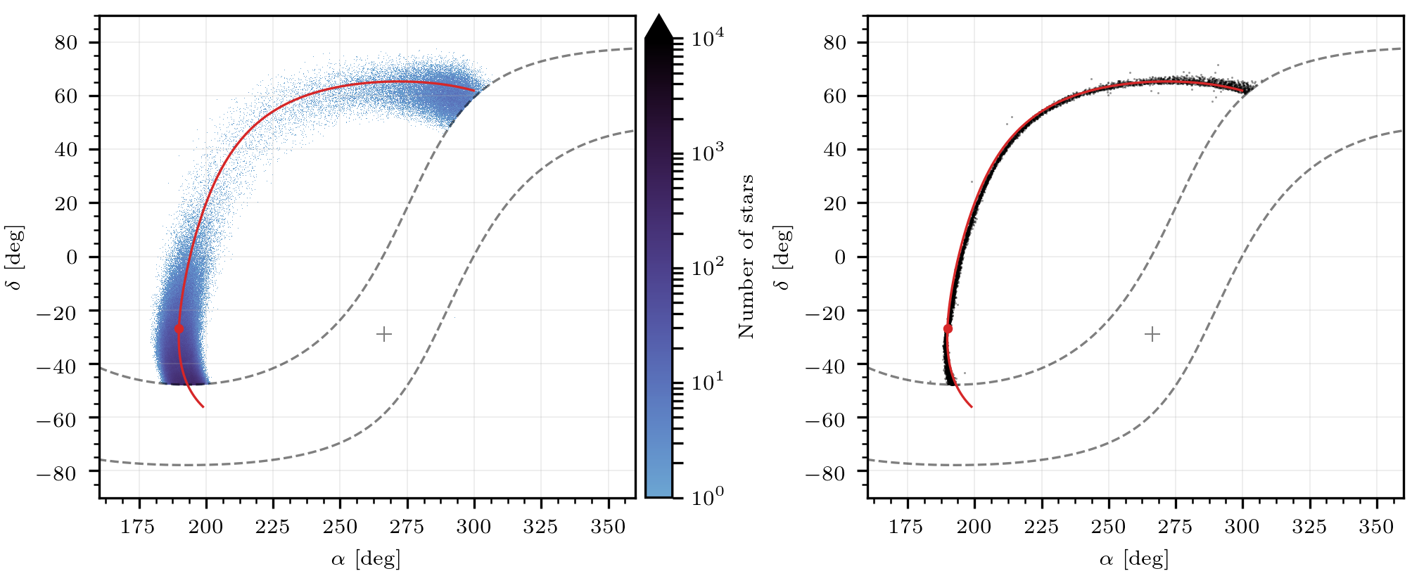 Figure 22
 Figure 23
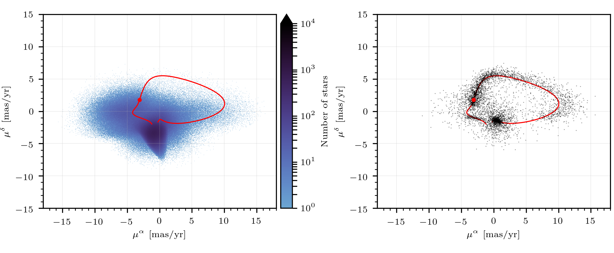 Figure 24
 Figure 25
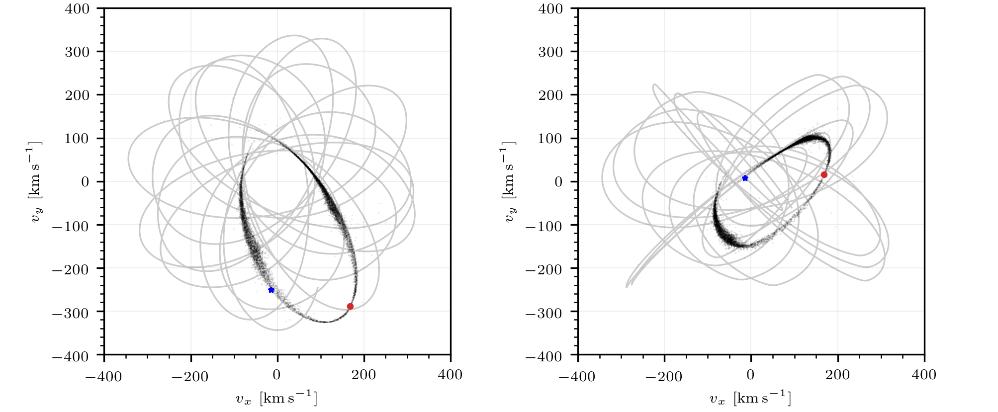 Figure 26
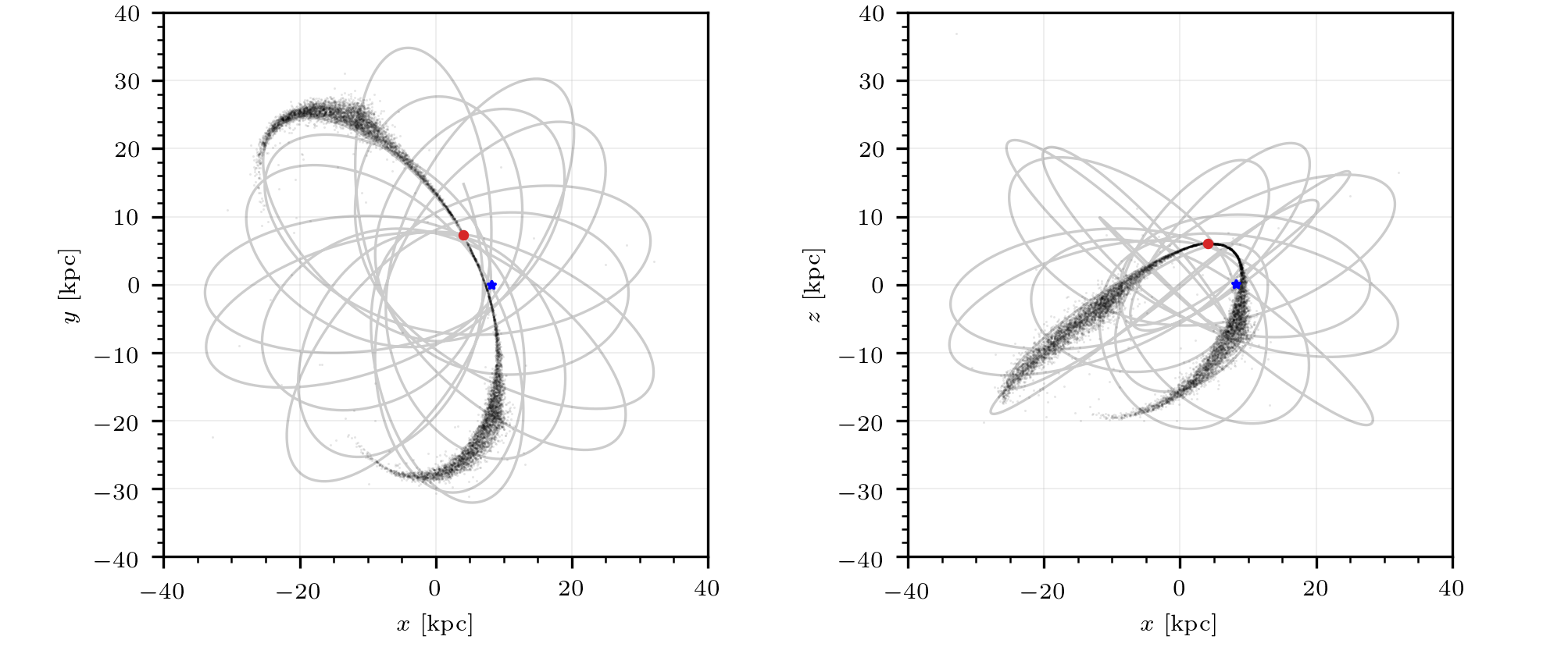 Figure 27
| Properties | Thin disc | Thick disc | |
|---|---|---|---|
|
(M⊙ kpc-2) |
|||
|
(kpc) |
|||
|
(kpc) |
|||
|
(M⊙) |
|||
| Properties | Bulge | Stellar halo | Dark halo | |
|---|---|---|---|---|
|
(M⊙ kpc-3) |
||||
|
(kpc) |
||||
|
(kpc) |
||||
|
(M⊙) |
||||
|
(km s-1) |
(km s-1) |
(km s-1) |
(km s-1) |
|
|---|---|---|---|---|
| Thin disc | 31 | 12.6 | 20 | -229.4 |
| Thick disc | 67 | 42 | 51 | -185 |
| Bulge | 113 | 100 | 115 | -159 |
| Stellar halo | 131 | 85 | 106 | -12 |
| Properties M68 | Ref. | ||
|
(M⊙) |
[1] | ||
|
(pc) |
[1] | ||
|
(kpc) |
[2] | ||
|
(deg) |
[3] | ||
|
(deg) |
[3] | ||
|
(km s-1) |
[2] | ||
|
(mas yr-1) |
[3] | ||
|
(mas yr-1) |
[3] | ||
| Properties dark halo | |||
|
(M⊙ kpc-3) |
|||
|
(kpc) |
|||
|
(kpc) |
|||
|
(M⊙) |
|||
| Properties orbit | |||
|
(kpc) |
|||
|
(kpc) |
|||
|
(km s-1 kpc) |
|||
| Pre-selection cut | GOG18 | Stream stars | |
|---|---|---|---|
| All catalogue | 1510 398 719 | 33 228 | |
| (1) - (2) - (3) | 269 125 739 | 17 183 | |
| (4) | 613 098 | 6627 | |
| (5) | 612 909 | 6564 | |
| Pre-selection cut | GOG18 | GDR2 | |
| All catalogue | 1510 398 719 | 1692 919 135 | |
| (1) - (2) - (3) | 269 125 739 | 276 019 797 | |
| (4) | 613 098 | 446 982 | |
| (5) | 612 909 | 440 499 | |
| Region (i) Circle | |||
| (6) | 1 (1) | 13 | |
| (7) | 1 (1) | 13 | |
| Region (ii) Disc 1 | |||
| (6) | 6 (4) | 12 | |
| (7) | 2 (1) | 4 | |
| Region (iii) Halo | |||
| (6) | 17 (33) | 126 | |
| (7) | 17 (2) | 98 | |
| Final selection | |||
| (6) | 24 (38) | 151 | |
| (7) | 44 (4) | 115 | |
| Statistical parameters | |||
|---|---|---|---|
| Best-fitting kinematics of M68 | |||
|
(kpc) |
|||
|
(km s-1) |
|||
|
(mas yr-1) |
|||
|
(mas yr-1) |
|||
| Best-fitting parameters of dark halo | |||
|
(M⊙ kpc-3) |
|||
|
(kpc) |
|||
|
(kpc) |
|||
|
(M⊙) |
|||
| Derived orbital parameters of M68 | |||
|
(kpc) |
|||
|
(kpc) |
|||
|
(km s-1 kpc) |
|||
|
(mas) |
(deg) |
(deg) |
(km s-1) |
(mas yr-1) |
(mas yr-1) |
|
| 0.0971 | -26.75 | 189.87 | -94.7 | 1.7916 | -3.0951 | |
| 0.0023 | 2.5 | 2.5 | 0.2 | 0.0039 | 0.0056 | |
|
(M⊙ kpc-3) |
(kpc) |
(kpc) |
||||
| Globular Cluster | ||||
|---|---|---|---|---|
|
(deg) |
(deg) |
(deg) |
||
| NGC5466 | 28.5331 | 211.3614 | 0.08 | |
| M3 | NGC5272 | 28.3760 | 205.5486 | 0.2 |
| M53 | NGC5024 | 18.1661 | 198.2262 | 0.2 |
| NGC5053 | 17.7008 | 199.1124 | 0.2 | |
| M68 | NGC4590 | -26.7454 | 189.8651 | 0.3 |
| N | source_id |
|
|||||||
|
(mas) |
(deg) |
(deg) |
(mas yr-1) |
(mas yr-1) |
(mag) |
(mag) |
( yr3 deg-2 pc-1 mas-3 ) |
||
| 1 | 3496364826490984832 | ||||||||
| 2 | 3496397262084464128 | ||||||||
| 3 | 6133483847268997632 | ||||||||
| 4 | 3496359908751562496 | ||||||||
| 5 | 6129336321904932224 | ||||||||
| 6 | 3496403270742208768 | ||||||||
| 7 | 3496413819180463616 | ||||||||
| 8 | 6128205985298801408 | ||||||||
| 9 | 6153341199065073536 | ||||||||
| 10 | 3496363825761763840 | ||||||||
| 11 | 3496426983257641216 | ||||||||
| 12 | 3496351250097506816 | ||||||||
| 13 | 3496465702385628928 | ||||||||
| 14 | 3496383857489983232 | ||||||||
| 15 | 3496417912286695936 | ||||||||
| 16 | 3496385266239278976 | ||||||||
| 17 | 3692120708467214208 | ||||||||
| 18 | 3496354101955858432 | ||||||||
| 19 | 1606236095606481280 | ||||||||
| 20 | 1458389959637031296 | ||||||||
| 21 | 3677284104720388224 | ||||||||
| 22 | 3730942295084892928 | ||||||||
| 23 | 1455844345403174016 | ||||||||
| 24 | 3691856546503440128 | ||||||||
| 25 | 3675964587688060416 | ||||||||
| 26 | 1456842495802767744 | ||||||||
| 27 | 3678259474613592960 | ||||||||
| 28 | 3729366935440429952 | ||||||||
| 29 | 3678958794072858112 | ||||||||
| 30 | 3938507382917888512 | ||||||||
| 31 | 3730306639925232384 | ||||||||
| 32 | 3736013929907004928 | ||||||||
| 33 | 1504696231140527232 | ||||||||
| 34 | 3686001101624868352 | ||||||||
| 35 | 1605773136787896320 | ||||||||
| 36 | 3731064894927486976 | ||||||||
| 37 | 1455852248142764288 | ||||||||
| 38 | 3677590211334628992 | ||||||||
| 39 | 3677713562794613504 | ||||||||
| 40 | 1600425932567734784 | ||||||||
| 41 | 1603928701735870336 | ||||||||
| 42 | 3736784721917729152 | ||||||||
| 43 | 3939089398230332928 | ||||||||
| 44 | 1634945752956687104 | ||||||||
| 45 | 1505103084803276160 | ||||||||
| 46 | 3736463664522214656 | ||||||||
| 47 | 1506844779940816384 | ||||||||
| 48 | 3729915076346434304 | ||||||||
| 49 | 3678969243729036032 | ||||||||
| 50 | 3690547165593837312 | ||||||||
| 51 | 1496589879802806528 | ||||||||
| 52 | 1496266863902585728 | ||||||||
| 53 | 1496030911283208576 | ||||||||
| 54 | 1498889611451314816 | ||||||||
| 55 | 1604273437287099776 | ||||||||
| 56 | 3678292459962501376 | ||||||||
| 57 | 3685425060611225472 |
Peer Reviews
No public reviews on file for this paper yet. If you reviewed it on a platform where reviews are public (OpenReview, ICLR, NeurIPS, ICML), you can paste yours below so the community can read it here.
Videos
No videos yet. Explain this paper in a talk, walkthrough, or lecture? Add one.
Statistical detection of a tidal stream associated with the globular cluster M68 using Gaia data
Carles G. Palau,1 Jordi Miralda-Escudé,1,2,3
1Institut de Ciències del Cosmos, Universitat de Barcelona (UB-IEEC), Martí i Franquès 1, E-08028 Barcelona, Catalonia, Spain.
2Institució Catalana de Recerca i Estudis Avançats, E-08028 Barcelona, Catalonia, Spain.
3Institute for Advanced Study, Princeton, NJ 08540, USA E-mail: [email protected]: [email protected]
(Accepted XXX. Received YYY; in original form ZZZ)
Abstract
A method to search for tidal streams and to fit their orbits based on maximum likelihood is presented and applied to the Gaia data. Tests of the method are performed showing how a simulated stream produced by tidal stripping of a star cluster is recovered when added to a simulation of the Gaia catalogue. The method can be applied to search for streams associated with known progenitors or to do blind searches in a general catalogue. As the first example, we apply the method to the globular cluster M68 and detect its clear tidal stream stretching over the whole North Galactic hemisphere, and passing within 5 kpc of the Sun. This is one of the closest tidal streams to us detected so far, and is highly promising to provide new constraints on the Milky Way gravitational potential, for which we present preliminary fits finding a slightly oblate dark halo consistent with other observations. We identify the M68 tidal stream with the previously discovered Fjörm stream by Ibata et al. The tidal stream is confirmed to contain stars that are consistent with the HR-diagram of M68. We provide a list of 115 stars that are most likely to be stream members, and should be prime targets for follow-up spectroscopic studies.
keywords:
globular clusters: individual: M68 - Galaxy: halo - Galaxy: kinematics and dynamics - Galaxy: structure.
††pubyear: 2019††pagerange: Statistical detection of a tidal stream associated with the globular cluster M68 using Gaia data–E
1 Introduction
Tidal streams are a powerful method to constrain the Milky Way potential by dynamically modelling them and obtaining fits to their evolution as stars are released from the tidally perturbed progenitor. Several tidal streams have been discovered containing large numbers of stars, the majority of them from dwarf galaxies. The largest stream is produced by the Large Magellanic Cloud (Wannier et al., 1972), and the second is made by the tidal arms of the disrupting Sagittarius dwarf galaxy (Majewski et al., 2003); these streams may be affected by more complex physical processes including star formation in gas that is affected by ram-pressure as it moves through the Galactic halo hot gas. Other tidal streams do not have an obvious progenitor, such as the Orphan stream (Grillmair, 2006) and the Monoceros Ring (Newberg et al., 2002). Tidal streams were also discovered from the globular clusters Palomar 5 (Odenkirchen et al., 2001) and NGC5466 (Belokurov et al., 2006; Grillmair & Johnson, 2006). In addition, the GD-1 tidal stream, spanning about 60 deg on the sky, is believed to have originated from a globular cluster that was finally completely disrupted by the tidal perturbation (Grillmair & Dionatos, 2006). Additional cases of tidal tails have been reported which are more distant and of a lower surface brightness than previous ones (e.g. Grillmair, 2009), most of them recently discovered with photometry data of Dark Energy Survey (Balbinot et al., 2016; Shipp et al., 2018). A list of the streams detected up until 2015 and a summary of the techniques used for finding them is found in Grillmair & Carlin (2016).
As the number of discovered tidal streams grows and the accuracy of the measured motions of stars within them is improved, increasingly accurate constraints on the Milky Way potential should be derived by requiring a match of the dynamics of all streams. Several methods have been designed for this purpose (Varghese et al., 2011; Bonaca et al., 2014; Price-Whelan et al., 2014). One of the most notable applications of these streams that has been discussed is the creation of density variations and gaps along tidal streams from tidal interactions with perturbing satellites moving across the Milky Way halo, including the predicted dark matter sub-haloes (Carlberg, 2009). The Cold Dark Matter model should in principle make reliable predictions for the abundance and shape of any such gaps in tidal streams, although other objects such as globular clusters and molecular clouds may give rise to similar features (Carlberg & Grillmair, 2013; de Boer et al., 2018). For all these reasons, a strong interest has developed in detecting as many streams as possible. The publication of the Gaia Data Release 2 (GDR2), with proper motions and parallaxes of unprecedented accuracy, is a giant step forward in our ability to discover, analyse and model large numbers of tidal streams in the Milky Way (Ibata et al., 2018; Malhan et al., 2018; Price-Whelan & Bonaca, 2018).
Globular clusters are an important class of objects that should, in general, be accompanied by tidal streams. At each passage through the galactic pericentre and at each crossing of the disc, the tidal perturbation reaches a maximum and causes a peak in the rate at which stars are tidally pulled out of the system into unbound orbits, populating the leading and trailing tails. The streams, however, may be of very low density and difficult to detect. Apart from tidal truncation, globular clusters also evolve under internal dynamical relaxation and mass segregation, which preferentially diffuses low-mass stars into outer orbits from which they can be tidally perturbed and incorporated into the tidal tails. This selection favouring low-mass stars in tidal tails can make them more difficult to detect in flux-limited surveys (Leon et al., 2000; Balbinot & Gieles, 2018).
So far, tidal tails have often been found serendipitously by simply noticing an excess of stars along bands in the sky after applying certain cuts based on proper motions and photometry. With the massive amount of new data coming from the Gaia mission, there is a need to optimize and systematize detection methods of tidal streams to ensure that they are efficiently found. Several methods have been proposed to find them from large samples of stars with phase-space coordinates, magnitudes, and colours:
- •
Brown et al. (2005) try to identify tidal streams on the energy-angular momentum plane. This method needs an axisymmetric potential for the Galaxy and requires high-quality data because the large background population and the observational uncertainties make difficult the detection of a stream as a single structure projected on only two integrals of the motion, even with Gaia data.
- •
Sanderson et al. (2015) integrate orbits in a specific potential model of the Galaxy, and then search for streams in the angle-action space using a clustering algorithm. This method tends to suffer from similar problems as the previous method when using an oversimplified potential model that scatters the real stream members over an excessively large region of phase space.
- •
Mateu et al. (2017) use an algorithm (Great Circle Method) exploiting the fact that streams are confined to a plane if the Galaxy potential is close to spherical, searching for stars with positions and proper motions that approximately lie in a unique plane. The problems are similar to the previous methods when the potential is not very close to spherical and parallax errors introduce uncertainties in determining the plane of the star orbits.
- •
Finally, Malhan & Ibata (2018) present an algorithm, called Streamfinder, designed to find distant halo streams, where a six-dimensional tube in phase space that follows the orbit of a star computed in a fixed potential is constructed with a width similar to the size of the expected stream. A large number of observed stars that are compatible with this tube, taking into account the errors of the measurements, is then an indication of the reality of a putative stream.
Here we present a new method based on maximum likelihood analysis that searches for streams in a large data set, computing orbits in a gravitational potential that can be varied together with the kinematic initial conditions of a stream progenitor. The method takes into account the probability density of stars to belong to a model of the stellar foreground and to belong to a tidal tail, and can be applied for known candidate progenitors or for blind searches with unknown progenitor orbits. The search for a stream is done after a pre-selection that eliminates most of the stars in the data set that are very unlikely to belong to any tidal stream in the phase-space region being searched, which is used to reduce computational time. Among previous stream detection methods, our one resembles the most the Streamfinder method of Malhan & Ibata (2018), improving and generalizing the likelihood function using a model of the phase-space density of the Milky Way for the stellar foreground and a variable gravitational potential, and a realistic dynamical treatment of a tidal stream taking into account the intrinsic and observational uncertainties at the pre-selection and best-fitting stages.
This type of method has so far not been exhaustively applied to the list of known globular clusters. In this paper, we develop this method to search for tidal tails around a known progenitor, with the goal of identifying them even though they will generally not be intuitively visible to the eye as an excess under any projections and cuts and can only be detected as a statistical excess above the foreground or background stars with known observational errors. We apply the method specifically to the globular cluster M68 (NGC4590) in this paper, because of several characteristics that make it the best candidate for observing any associated tidal stream. We find clear evidence of a long stream with more than 100 member stars that promises many applications for studies of the Galactic potential and the dynamics of tidal stream formation.
As this work was being completed, we became aware111 We thank Daisuke Kawata for pointing this out to us and for many inspiring comments on our work that the stream we detect was already discovered in Ibata et al. (2019), who baptized it with the name Fjörm; however, they did not associate it with the globular cluster M68. We find incontrovertible evidence for this association, which makes this stream even more interesting for studies of the dynamics of globular clusters and the Milky Way potential.
Our method is described in detail in Section 2, and Section 3 presents tests on simulations of the Gaia catalogue, applying them specifically to stream models of M68. In Section 4, we search for a real stellar stream associated with M68 using Gaia data and we present our conclusions in Section 5.
2 Statistical method to detect tidal streams
In this section we describe the method we have developed to search for tidal streams. Our goal is to be able to detect a tidal stream even when seen against a large number of foreground stars with similar kinematic characteristics, and when large observational errors on the distance and proper motions and the absence of radial velocities make it difficult to visualize the tidal stream directly from any projection of the data. In many cases, there may be no individual stars that can be assigned to a tidal stream with high confidence, even though the existence of the tidal stream itself may be highly significant from a large set of candidate members. The method is based on the maximum likelihood technique, although the likelihood function has to be defined in an approximate way because of the difficulty of numerically computing precise distributions of a tidal tail for many models, and of correctly characterizing the foreground. The approximations used are tested and calibrated using mocks of the Gaia data.
Stars in a tidal stream are stripped out from a bound object (a globular cluster or a dwarf galaxy) by the external tidal force of the Milky Way galaxy. Tidal stripping occurs when the mean density of the Galaxy within the cluster orbit is comparable to the mean cluster density, which also implies that the orbital times of the stripped stars in the cluster are comparable to the orbital time of the cluster around the Galaxy. Tidal stripping is therefore strongest at the closest pericentre passages. In addition, tidal shocks occur when the cluster crosses the disc. The escaped stars approximately follow the progenitor orbit, with small variations of the conserved integrals of the motion. Stars moving to lower orbital energy form a leading tail ahead of the cluster trajectory, while stars left at a higher orbital energy form a trailing tail behind. The shape of these tails is a first approximation to the cluster orbit, although in detail, they are different (Küpper et al., 2010; Bovy, 2014; Fardal et al., 2015).
2.1 Likelihood function and parameter estimation methodology
The maximum likelihood method is used to determine parameters of a model that maximize a posterior function, given a set of observational data. The likelihood function is the probability density of obtaining the observed data as a function of the model parameters. The data generally consist of independent observations of a set of variables (labelled by an index ), with a covariance matrix for observational errors . We want to compute a probability density P\mbox{\footnotesize(w^{\mu}|\theta_{\kappa};\sigma^{\mu\nu})} in the space of the variables, depending on model parameters (with ) that are to be estimated. The dependence on the covariance matrix is assumed to be a convolution with Gaussian errors, in the appropriately chosen variables. In our case, is the number of stars in a selected catalogue where we search for evidence of a tidal tail, are the observed coordinates of each star of parallax, angular position, radial velocity and proper motion, and the covariance can be different for every star. The likelihood function L\mbox{\footnotesize(\theta_{\kappa})} is the product of the probability densities of all the data points:
[TABLE]
A prior probability function p\mbox{\footnotesize(\theta_{\kappa})} is assumed for the parameters .
In addition to fitting parameter values, the likelihood function can be used to calculate a statistical confidence level to establish if a certain hypothesis is true or false. Usually a null-hypothesis states that the model parameters obey a set of restricting equations, meaning that the parameters lie in a sub-space of dimensionality , while the one-hypothesis asserts that the parameters do not obey the restrictions and are outside of this sub-space. Let the parameters and be the values that maximize the posterior function, defined as the product L\mbox{\footnotesize(\theta_{\kappa})}\,p\mbox{\footnotesize(\theta_{\kappa})}, with the restrictions and without them, respectively. The truth of can be tested using the likelihood ratio statistic , defined as:
[TABLE]
We use Wilks’ theorem (see e.g., Casella & Berger, 2002) to choose the criterion for favouring the null-hypothesis , where is computed from a conventionally chosen value of the probability of inappropriately rejecting the null-hypothesis when is actually true, using the equation
[TABLE]
where is the standard distribution with degrees of freedom. We shall use a confidence level throughout this paper, which for one degree of freedom implies .
In general, the stars of any set in which we search for a tidal stream contain a fraction of stars that belong to the tidal stream, and a fraction that belong to the foreground containing the general stellar population of the Galaxy (note that what we refer to as “foreground” stars may actually be foreground or background compared to the stream, and we simply mean that they are superposed in the sky with the hypothesized stream and belong to the set in which the stream is being searched for). The null-hypothesis is simply the restriction . The probability density of the data variables for each star is
[TABLE]
Here, is the probability density that a star belonging to the stream has variables , convolved with errors , while is the probability density for a star that belongs to the foreground. We have split the model parameters into three groups: refers to parameters of the distribution of stars in various components of the Galaxy (disc, bulge, and halo), are the present coordinates of the orbiting object generating the tidal stream, and are parameters of the Milky Way potential. In general, the parameters also affect the potential if the stellar components are assumed to imply a mass component with the same distribution (i.e., if a fixed mass-to-light ratio of the stellar population is assumed), so we include these parameters in as well. The likelihood function is then given by equations (1) and (4). The values of the parameters for which the likelihood function is maximum are computed using a Nelder-Mead Simplex algorithm, which does not require neither a smooth function nor the evaluation of its derivatives (see Conn et al., 2009, for details). The covariance matrix for the errors of the parameter solutions are computed by calculating second derivatives of the posterior function logarithm
[TABLE]
The stellar phase-space density model depending on parameters is described in detail in Section 2.2, and the calculation of taking into account an observational selection approximation is explained in Section 2.4. The computation of the probability density from a density model of the stream, using the stream progenitor orbit and a model of the Milky Way potential, is described in Section 2.5.
We have not included information about colours and magnitudes of the stars in the likelihood function since it would be necessary to model the colour-magnitude distribution of the foreground stars as seen by Gaia. Although the inclusion of photometric data might improve the detection capability, we leave this modification for future further improvement of the statistical method. In Section 3, we use the phase-space data to establish the existence of a simulated tidal stream and to compute the best adjustment of the model parameters using a foreground simulated star catalogue. We use colours and magnitudes in Section 3.5 to improve the final identification of the star candidates to belong to the stellar stream choosing those that are compatible with the HR-diagram of the progenitor cluster.
2.2 Phase-space stellar model of the Milky Way
We define a simple model of the phase-space distribution of stars in the Milky Way, , to enable an estimate of the probability density that a star belongs to the Galactic foreground, . The distribution in our model is the sum of four components: thin disc, thick disc, bulge and stellar halo. We write each of the four components, labelled by the index , as the product of a stellar mass density function of space, , and a velocity distribution function :
[TABLE]
where and are three-dimensional components of position and velocity vectors, and is the total mass of stars in the four components. The velocity distribution is normalized to unity at each position , when integrating over all the velocity space. We make the simplified assumption that the number of stars per unit stellar mass at a given luminosity in the Gaia band is the same for all components.
2.2.1 The disc density
The disc is constructed as the sum of two exponential profiles, for the thin and thick disc. In cylindrical coordinates , the mass density for each component is
[TABLE]
We use the parameter values in McMillan (2011), which are listed in Table 1.
2.2.2 The bulge density
For simplicity we assume an axisymmetric bulge, even though the bulge is a rotating bar, since our conclusions in this paper do not depend on accurately modelling orbits in the inner part of the Galaxy. The bulge density is a power law with slope and a Gaussian truncation at a scale length :
[TABLE]
where
[TABLE]
The bulge parameters are listed in Table 2, taken from McMillan (2011).
2.2.3 The stellar halo density
The Galaxy is surrounded by a faint stellar halo made by old and metal-poor stars. We model it as an oblate ellipsoidal object with a density profile as a function of the radial variable in equation (9) following a two power-law model:
[TABLE]
We use the parameters of Robin et al. (2014), listed in Table 2.
2.2.4 The velocity distribution model
For all the stellar components, we assume that the velocity distribution function is a Gaussian with principal axes oriented along spherical coordinates,
[TABLE]
where the index labels the four stellar components. The three-velocity dispersion eigenvalues are determined observationally. We use the values for each component from Robin et al. (2012), assuming the average of all stellar populations for the thin disc. The values are listed in Table 3.
2.3 Potential model of the Milky Way
We assume the dark matter halo density profile also follows equation (10). For the case and , this density profile reduces to the NFW profile (Navarro et al., 1996), which fits the dark matter halo profiles obtained in cosmological simulations. For simplicity we also assume an axisymmetric shape for the dark halo, even though in general it can be triaxial. In the models in this paper we fix and we leave the other parameters listed in Table 2 to be free when fitting the model. In practice this gives enough freedom to our halo profile to model the dynamics of tidal tails we examine here.
Two baryonic components are added to this dark halo: the disc and the bulge. Their potentials are computed following the previous stellar density profiles in equations (7) and (8). The stellar halo and gas components are neglected because of their expected small mass compared to the dark halo.
2.4 The probability function
In general, stellar surveys provide measurements of phase-space coordinates of stars in the form of parallaxes , angular positions and , radial velocity , and proper motions and . These are our six-dimensional variables for each star, , where the proper motions are and . Note that the physical proper motion component in right ascension is . The Gaia mission is at present providing the largest star survey. We designate as the observed value of each variable, and their observational errors are characterized by a covariance matrix . The values of the true variables are assumed to follow Gaussian distributions that we write as .
To calculate the probability density of the observed coordinates for foreground stars, we need to take into account the flux-limited survey selection. Let \psi_{\rm s}\mbox{\footnotesize(L)} be the cumulative luminosity function of stars with a luminosity in the observed photometric band greater than . Neglecting the effect of dust absorption (which generally has small variations for the halo stars we are interested in), the density of stars included in the survey as a function of the heliocentric distance is proportional to \psi_{\rm s}\mbox{\footnotesize(L_{1}r_{\rm h}^{2}/r_{1}^{2})}, where is the luminosity corresponding to the survey flux threshold at a distance . We can take the normalizing distance to be 1 parsec, and then the parallax expressed in arc seconds is . We will assume here as a simple model that \psi_{\rm s}\mbox{\footnotesize(L)}\propto L^{-1} in the range of interest, meaning that there is a roughly constant luminosity coming from stars in any range of . This is roughly correct for stellar populations lying between the main-sequence turn-off and the tip of the red giant branch. A detailed modelling of the foreground to obtain an accurate estimate of the likelihood function would clearly require a more careful evaluation of the stellar luminosity function, but given all the uncertainties in our modelling (i.e., the velocity distribution, dust absorption, etc.) we decide to use this very approximate and simple approach in this work.
The foreground probability density can then be written as
[TABLE]
where the Jacobian of the transformation from the cartesian variables of phase space to the coordinates has a space part , and a velocity part . The constant renormalizes the probability density in the observed variables after the flux-threshold selection is included, and is
[TABLE]
For our choice \psi_{\rm s}\mbox{\footnotesize(L)}\propto L^{-1}, the function is simply replaced by in equations (12) and (13).
We now assume that the observational errors are dominated by the parallax error and the radial velocity , neglecting errors in proper motion compared to the intrinsic velocity dispersion of stars. Errors in the angular positions are always negligibly small. The integral yielding our foreground probability density is then
[TABLE]
In the absence of any radial velocity measurement, we can simply use a very large value of , or redefine the probability by integrating over all radial velocities. Our assumption of small proper motion errors is not always valid, and in this case, an improved estimate needs to integrate over the full three-dimensional velocity distribution.
The integral in equation (14) is computed numerically, converting the observable coordinates to heliocentric cartesian coordinates and Galactocentric ones as described in Appendix A to evaluate f\mbox{\footnotesize(w^{\mu}|\theta_{s})}.
2.5 The probability function
The most accurate way to model tidal streams is through direct -body simulations. However, these require the introduction of a softening radius when particles are a random representation of collisionless matter instead of real stars. Including a sufficient number of particles to model the evolving gravitational potential of the globular cluster and its tidal tail would increase the computational time by more than a factor even with the use of a tree-code or other techniques. In addition, we should include the perturbation on the Milky Way potential by the globular cluster because it would be of similar importance, thus increasing the computational requirements of the model. In practice, we need to compute the trajectories of thousands of stars in a tidal tail, and to repeat the calculation for hundreds of models to minimize the likelihood function and to obtain a fit. To make this computationally feasible, we neglect the self-gravity of the stream and compute test particle trajectories in the fixed Milky Way potential plus the fixed potential of the satellite system orbiting around the Milky Way, neglecting any dynamical perturbation on the satellite and on the Milky Way.
Based on these simplifications, a wide range of studies are based on releasing test particles near the Lagrange points, with a random offset in position and velocities following Gaussian distributions (see e.g., Lane et al., 2012). This method reasonably reproduces -body simulations with a large reduction in computational time, and has been studied in detail in Küpper et al. (2008) and in Küpper et al. (2012). The potential of the progenitor is sometimes not taken into account in these simulations, even though its effects can be significant, as was shown for example in Gibbons et al. (2014).
In this work, we use neither -body simulations because of their impractical computational demand, nor the above-mentioned algorithms because we want to simulate the kinematic structure of streams in a general orbit and general potential for the Milky Way. We simulate trajectories of test particles including an unperturbed potential for the progenitor system, following these steps:
Compute backwards in time the orbit of the progenitor globular cluster (or other bound satellite) from a reasonably well-known present position and velocity. 2. 2.
Spread out stars around the globular cluster using a model derived from its internal stellar phase-space distribution function. 3. 3.
Compute forwards in time the orbits of the stars within the potential of the Galaxy, including the moving potential of the globular cluster with its mass fixed. 4. 4.
Use the stars that have escaped from the progenitor to create a model of the phase-space density of the stellar stream.
2.5.1 Simulation of the tidal stream
We generally refer to the stellar system being tidally stripped as a globular cluster, although tidal streams can of course be formed by any stellar systems orbiting around our Galaxy. We assume the globular cluster is initially in dynamic equilibrium, spherical, and with an isotropic velocity dispersion, and adopt the Plummer Model for its internal structure, with two parameters: the total cluster mass and a core radius . The density profile as a function of the distance to the cluster centre, , is
[TABLE]
The velocity distribution at any radius can be expressed in terms of the modulus of the escape velocity,
[TABLE]
where the gravitational potential is
[TABLE]
The probability distribution of the modulus of the velocity is
[TABLE]
We first compute orbits for a large number of test particles with random initial conditions, obtained by generating an initial radius according to the density profile of equation (15), a velocity modulus according to equation (18), and two random angles for the position from the cluster centre and for the velocity vector. The orbits of the test particles are computed in the combined potential obtained by adding that of the Milky Way (as described above) and that of the cluster Plummer model in equation (17). The orbit of the globular cluster in the Milky Way potential is computed first, also as a test particle and stored. The test particles are computed next by considering the cluster potential to be fixed in shape (neglecting the changes in the mass distribution caused by the tidal perturbation) and moving along the computed orbit.
A technical problem appears because most of the particles generated in this way have orbits close to the cluster core, which is typically much smaller than the tidal radius of the cluster, leaving only a very small fraction of stars that can escape. Moreover, integrating the trajectory of test particles near the cluster core is computationally expensive because orbital periods in the cluster core are usually much shorter than the orbital period around the Milky Way, so many short time-steps are required. To avoid this problem, we restrict the generated test particles to a subset representing cluster stars that are more likely to escape than the majority, while making sure that particles that are not selected would very rarely escape and not significantly contribute to stars in the simulated tidal tail.
Although it is not possible to determine analytically if a star in a model cluster with any orbit is able to escape, we can obtain an approximate restricted region of phase space where most escaping stars should be located. For this purpose, we consider the restricted circular 3-body problem of a cluster in a circular orbit, where the combined potential is time independent in the rotating frame following the cluster motion. Considering a characteristic cluster orbital radius , the distance between the centre of the cluster and the first Lagrange point (see Renaud et al., 2011) is approximately given by the tidal radius:
[TABLE]
With respect to the rotating reference frame where the two bodies are at rest, the movement of a test particle can be described adding an extra term to the potential needed to account for the centrifugal force giving the following effective potential in spherical Galactocentric coordinates:
[TABLE]
where is the gravitational constant and is the potential of the Milky Way. Using the theorem of conservation of energy, we define a limiting velocity taking a fixed radius :
[TABLE]
For the simulation of the density of a tidal stream we use a sample generated via a Monte Carlo method taking only the stars with initial velocity such that and . The stars of the globular cluster are considered test particles and their orbits are integrated using a Runge-Kutta scheme from the past to the current position within the potential of the Milky Way and within the potential of the globular cluster keeping its mass constant.
2.5.2 Density model of the tidal stream
Once the orbits of the stars are computed, we construct a probability density function of the tidal stream in the space of the directly observed variables , designated as p_{\scaleto{\rm S}{3.5pt}}\mbox{\footnotesize(w^{\mu}|\theta_{s},\theta_{c},\theta_{\phi})}. We use a Kernel Density Estimation method, with a Gaussian as a kernel. If is the total number of escaped stars at the present time, the stream probability density is
[TABLE]
The centre of each Gaussian distribution, , is the current position of the simulated stream star, and the covariance matrix is computed from the distribution of positions of neighbouring stream stars, using weighting factors that average over neighbours out to some characteristic kernel size:
[TABLE]
The weights are defined depending on the distance between every pair of stream stars,
[TABLE]
where are the Cartesian space coordinates of each stream star at the present time in the simulation. We have tested that a value and the exponent in the previous equation gives a reasonable reproduction of the shape and density profile of the stellar stream, and we use these values in this work. These quantities can, however, be varied to optimize any specific application of the method.
Note that although we use the physical distances to compute the kernel weights, the stream structure is modelled in the space of directly observed coordinates . The probability density that we model as the sum of Gaussians in equation (22) is therefore the product of a phase-space density times the Jacobian to transform from phase-space Cartesian coordinates to the variables of the observations.
2.5.3 The probability function
We can now write the probability density that a star belonging to the stream and following the distribution as modelled in Section 2.5.2 is observed to have the variables :
[TABLE]
We assume that the dispersion of the stream is much smaller than the parallax observational error of a star, i.e., , to approximate \psi_{\rm s}\mbox{\footnotesize(\pi)}\simeq\psi_{\rm s}\mbox{\footnotesize(\pi_{{\rm c}i})}. In this case the integral in equation (26) is easily performed because the convolution of two Gaussians is a Gaussian with the sum of the dispersions. Using this result, the probability of a star to have the observed position with observational errors , assuming it is a member of the stream, is
[TABLE]
where the normalization constant is:
[TABLE]
2.6 Definition of the prior function
We use the prior function given by the direct observational measurements of the distance, proper motions and radial velocity of M68, with their quoted errors, as given in Table 4 below. These four globular cluster orbit parameters, labelled as with , follow Gaussian distributions:
[TABLE]
with observed values and uncertainties listed in Table 4. We assume a flat prior for the four gravitational potential parameters of the dark halo in the same table.
Given the values that maximize the posterior function in equation (2), the deviation with respect to the observed measurements can be quantified by
[TABLE]
A value of substantially larger than the number of parameters 4 would mean that the fit to a detected stream is not consistent with the measured distance and velocities of the globular cluster progenitor, indicating perhaps an inadequate potential parameterization or an underestimation of the errors.
3 Validation of the statistical method
In this section we simulate the tidal stream of a globular cluster and the way it can be observed in the Gaia survey to test if our algorithm is able to detect the stream against a simulated foreground and recover some of the parameters of the progenitor orbit and the gravitational potential in which the stream moves.
3.1 Description of the simulated Gaia catalogue
We start describing a simulation of the entire Gaia catalogue that we then use to generate a realistic set of foreground stars that a tidal tail would be observed against.
The Gaia Universe Model Snapshot (GUMS) is a simulated catalogue of the full sky Gaia survey for stellar sources, which is useful for testing many types of statistical studies. Based on Besançon Galaxy model (Robin et al., 2003), the simulation includes parallaxes, kinematics, apparent magnitudes, and spectral characteristics for billion objects with magnitude mag. A complete statistical analysis of the 10th version of this catalogue is found in Robin et al. (2012).
The Gaia Object Generator (GOG) is a simulation of the contents of the final Gaia catalogue based on the sources in the GUMS, and provides the Gaia expected measurements of astrometric, photometric, and spectroscopic parameters with observational errors based on the Gaia performance models222https://www.cosmos.esa.int/web/gaia/science-performance. These estimated observational errors depend on instrument capabilities, stellar properties, and the number of observations. A statistical analysis of this catalogue was presented in Luri et al. (2014). We use the 18th version of this simulation333https://wwwhip.obspm.fr/gaiasimu/ (GOG18) in this work.
The GOG18 simulates the end-of-mission Gaia catalogue, so the predicted errors are smaller than in the current available version (GDR2). We correct the GOG18 uncertainties by scaling them to make them applicable to the GDR2 catalogue. Given the simulated observational error of the phase-space coordinates, we obtain the scaled uncertainties , where the scale factor is computed to match the resulting distribution of simulated errors to the real distribution of GDR2 errors. For the variables , we find the required six scale factors to be
[TABLE]
Radial velocities are most frequently not available, and in this work we simply set the error to a large enough value to make our results insensitive to it. We choose km s*-1* and then, we set the observed value of the heliocentric radial velocity to zero for all stars (this value is irrelevant when the radial velocity error is large enough); we have tested that this value of is large enough that our results are not affected.
3.2 The M68 globular cluster and its tidal stream
Among several globular clusters we have considered as targets for a search for associated tidal tails, M68 (NGC4590) stands out because of its proper motions and distance are measured with good precision, it is projected on to the halo, its relative proximity to us, and a predicted orbit that brings it close to us and keeps it far from the inner region of the Galaxy. All these properties make any putative tidal tail easier to find: a long orbital period far from the Galactic centre means that the tidal tail has not been strongly broadened and dispersed by phase mixing, and a small distance to at least part of the tidal tail allows us to discover member stars of relatively low luminosity, especially if the foreground is far from the plane of the Galactic disc. After going through the list of known globular clusters, we selected M68 to be the most promising candidate for finding an associated tidal tail for these reasons.
The parameters for the computed orbit of the globular cluster M68 in our model of the Galactic potential are listed in Table 4, including its pericentre, apocentre, and angular momentum component perpendicular to the Galactic plane. As with other globular clusters, the proper motion measured by Gaia has dramatically improved the precision of the predicted orbit, which has been computed for several potential models (Gaia Collaboration et al., 2018b). In all the models the obtained orbit has an apocentre kpc, pericentre kpc, and a radial period of Myr, producing an elongated stream with little phase mixing and breadth. The globular cluster is approaching us and will come within kpc of the present position of the Sun in about 30 Myr, at the time when it is near its pericentre, flying almost vertically above our present position. This implies that any tidal tail should have a leading arm along this future part of the orbit, extending over the northern Galactic hemisphere, with the trailing arm being more difficult to see because of its position closer to the Galactic plane and further from us.
3.2.1 Simulation of the M68 tidal stream
To simulate the tidal tail produced by M68, we use the Milky Way dark halo model described by equation (10) with parameters listed in Table 4, corresponding to a total mass M⊙ and an axial ratio , and an implied potential flattening at the position of M68. The baryonic components of the mass distribution are added as described in Section 2.3.
The tidal stream is simulated following the steps described in Section 2.5, without applying the cuts in the simulated test particles described at the end of Section 2.5.1. These cuts are only applied later when the tidal tail needs to be computed for many models and the required computational time needs to be reduced. The orbit of M68, with properties listed in Table 4, is shown as a grey curve in Fig. 1 in two projections in space and two projections in velocity space. The blue star indicates the present position of the Sun and the red circle is the present position of M68. We calculate the orbits of a total of test stars, out of which 68 839 escape the potential of the globular cluster and form the tidal tail, shown in Fig. 1 as black dots. The simulation is run over 10 Gyr, first retracing the orbit of the globular cluster backwards in time and then calculating the orbits of the test stars starting with the initial conditions of the Plummer model 10 Gyr ago. At the beginning of the simulation, many stars are released because no radial cut-off is imposed on the assumed Plummer model in the initial conditions. The first pericentre passage and disc crossings also release many stars, but the rate of escape is reduced later once the globular cluster has already been stripped. For this reason, more stars are produced at the edges of the tidal tails, which also broaden with increasing distance from the cluster. This large number of stars released in the first orbits is a feature that obviously depends on the history of the cluster and the Milky Way, which our model does realistically predict. The part of the tidal tail closer to the cluster, released at later times, should be more realistic because it is produced after the cluster has already reached a steady rate of escaping stars.
Among the cluster stars generated according to the initial conditions of equations (15) and (18), the fraction of escaped stars at the end of the 10 Gyr simulation is shown in Fig. 2. This figure shows that our criterion to select only stars that are likely to escape (, shown as the red line), used in later simulations, is adequate to include most of the stars in the cluster that will actually be released in the tidal tail.
3.2.2 Simulation of the Gaia observational uncertainties for
stream stars
We now include realistic observational uncertainties in the simulated stream stars according to the expected measurement errors in the Gaia mission. We apply this to the total number 68 839 of escaped stars in our simulation to simulate the observed tidal tail. Naturally, the total number of stars in the tidal tail is highly uncertain, but our estimate of the number of available stars can be a reasonable one to the extent that the total number of globular cluster stars we have simulated is comparable to the expected number of stars in M68, and that the rate of escaping stars is also reasonable.
The Gaia observational uncertainties for the stream stars have been simulated using the Python toolkit PyGaia555https://pypi.org/project/PyGaia/, which implements the Gaia performance models. Observational errors depend on the Gaia magnitude, the Johnson-Cousins magnitude, the colour index , and the spectral type of each star. These magnitudes have been simulated as follows:
Assign randomly to each star a absolute magnitude and a colour index following the HR-diagram of M68 that we show in Fig. 3, which we have generated using 2929 GDR2 stars (see Appendix B). 2. 2.
Compute the colour index and the magnitude from the following approximations (Jordi et al., 2010), valid in the range :
[TABLE]
[TABLE] 3. 3.
Determine the spectral type using the effective temperature approximation (Carrasco et al., 2019):
[TABLE] 4. 4.
Compute the apparent and magnitudes of the stream stars, neglecting the dust extinction, and correcting the generated magnitude and the previously computed magnitude from the heliocentric distance of the globular cluster , to the heliocentric distance of the stream star.
The PyGaia functions give the end-of-mission Gaia errors, so we correct them by multiplying by the scale factors (equation 30). The simulated observed coordinates of stream stars, , are generated by adding a random Gaussian variable with dispersion to the true coordinates. The GDR2 measurements generally cannot be performed on stars fainter than , so only stars are included in our simulated catalogue of stream stars. In addition, the small number of simulated bright stars satisfying and are given a radial velocity with the Gaia observational error.
The resulting quantity of simulated stream stars after these cuts is 33 228, and is shown in the top row of Table 5 as the total number of stream stars in our simulated catalogue before we apply a number of pre-selection cuts that we describe next.
3.3 Data pre-selection
We now imagine that we have a catalogue with all the stars in the GOG18 simulation (a total of billion), and that includes in addition some fraction of our 33 228 simulated stream stars. Our method needs to detect the presence of the stellar stream in an optimal way and to identify the most likely candidate members.
To speed up the computation of the likelihood function and reduce the number of foreground stars of the final selection, most of which are in sky regions of high stellar density and far from the possible stream associated with M68, we apply a set of pre-selection cuts to the star catalogue. The stars that fulfil the following conditions are pre-selected:
- (1)
, to eliminate faint stars with large astrometric errors. 2. (2)
, e.g. large distance, to eliminate foreground disc stars. 3. (3)
, to avoid the regions of high stellar density close to the disc
For our fourth condition (4), we use a more complex pre-selection method to further restrict the number of stars that are used to evaluate the likelihood function for different stream models. The goal is to eliminate most of the foreground stars that can be ruled out as members of any possible stream associated with M68, within the uncertainties of the M68 orbit arising from observational errors and the Galactic potential. Our pre-selection method is described in detail in Appendix C.1; here we explain its basic idea, which uses the fact that the tidal stream is close to the orbit of the progenitor. We use a range of parameters for the orbit of M68 and the potential of the Milky Way to compute a bundle of possible orbits of M68 during the time interval from to , where is the present time and is chosen to obtain the relevant part of the orbit for the stream. Our simulations show that results in an adequate coverage of the reliable part of the stream in the case of M68, and we adopt this value in this paper. Many of the stars that are released by the cluster in the first few orbits, when the rate of escaping stars has not yet settled to a steady state, are located further from the globular cluster than this section of the orbit, and they are eliminated from the final catalogue in this fourth pre-selection condition.
The bundle of orbits computed in this way is used to define a region in phase space where stars have to be located to be pre-selected, also taking into account the observational errors. This is done by characterizing the bundle of orbits by a series of Gaussians, which are convolved with the Gaussians of observational errors. Stars have to be located within this region (involving conditions of the sky positions, proper motions, and parallaxes) to be pre-selected.
As the final fifth step (5), we remove stars that are within an angular distance of the globular cluster that gives rise to the tidal tail, and also stars in any other globular clusters that are within the pre-selected region, since they have highly correlated kinematics. The list of globular clusters that have been removed in this way are shown in Appendix C.2.
The number of stars in GOG18 and in the simulated stream of M68 after each one of these cuts is specified in Table 5. The first three steps reduce the general GOG18 catalogue by a factor close to six, and a smaller factor for the stream stars which are all sufficiently far from us and mostly at high Galactic latitude. The fourth step achieves the largest reduction in the number of foreground stars, a factor , by restricting the stars we look for to be consistent with our range of models in sky position, proper motion, and parallax. The stream stars are reduced by a factor of nearly 3, mostly due to the stars ejected in the first few orbits in the simulation that are near the edge of the stream, with a distribution that we consider as insufficiently reliable. The fifth step eliminates a very small fraction of stars, and is important mostly to remove stars that are bound or very close to M68.
The distribution of pre-selected stars in the GOG18 catalogue is shown as blue dots in the left-hand panels of Fig. 4, and the pre-selected stream stars are shown as black dots in the right-hand panels. Top panels show angular positions and bottom panels show proper motions. The tidal stream of M68 is particularly favourable to be observed because of the long stretch of the orbit that is close to us in a region of low foreground stellar density in the position and proper motion space.
3.4 Recovery of the dark halo parameters
We now test the detection of a tidal stream in the GOG18 simulated data set by adding a number of stars selected randomly among the 6564 stars of our simulated tidal stream. We find the maximum of the function described in Section 2.1 (equation 2), with the prior in equation (28) that incorporates the measurements of the M68 kinematics, when the parameters (fraction of tidal stream stars in the data set), (orbital parameters of M68), and (gravitational potential parameters) are allowed to vary. Each time we evaluate the likelihood for a new set of parameters, we need to resimulate the tidal stream and calculate the probability density of the stars with equation (22). To make this computationally easier, we calculate this stream probability density only for the fixed set of pre-selected stars described earlier, and we recompute orbits for the tidal stream only for a fixed set of 1200 test particles in the M68 globular cluster. These particles are selected among the ones with initial velocities and (see equations 21 and 19) using a mean cluster orbital radius kpc in equation (19), which increases the fraction of escaped stars and the efficiency of the calculation. Typically, the number of stars among these 1200 that escape M68 and form the tidal stream is about 1000, and is always greater than 750. We use these stream stars to recompute the smoothed phase-space density model of the tidal stream with equations (22) and (26), for each pre-selected star.
We find these number of stream stars is sufficient to obtain a reasonable accuracy for the best-fitting tidal stream. We note that choosing fixed initial conditions within the M68 Plummer model for the simulated stream stars as we vary the model parameters is important to ensure differentiability of the final stream star positions and velocities and a smooth likelihood function when we vary model parameters.
We compute the maximum likelihood and find the best-fitting stream model for a total of 30 cases: for six values of the number of stream stars added to the catalogue, , we do five independent cases with different random selections of stars among all the 6564 selected escaped stars in our base simulation of the M68 tidal stream (bottom row of Table 5).
Results are shown in Fig. 5. In each panel, the solid line connects the average results for the five cases of each value of , while the grey band is their range. The top panel shows the value of . When (shown as the horizontal dashed line), the detection of the stream is significant at the probability of rejecting the null-hypothesis. This happens always when , and in most cases for .
The second panel is the fraction of stream stars in the catalogue. The recovered fraction is generally lower than the true value (equal to the ratio of added stream stars to the total number of pre-selected stars), indicated by the dashed line. In general, can be different than the true value for two reasons: our foreground model is highly approximate and does not accurately reflect the distribution of stars in GOG18, and the stream phase-space density model we construct by adding Gaussians is also imprecise. The latter may explain the increasing ratio of the measured to the true with , if the algorithm tends to match the positions of a fraction of the stream stars while ignoring the rest at low .
The third panel is the value of from equation (29). This value is small when the detected stream does not impose significantly improved constraints on the globular cluster orbit compared to the prior (the measured proper motions, radial velocity, and distance), but grows as the stream stars provide more stringent constraints on the orbit. If , the detected stream is pushing the best-fitting orbit away from the measured values. Significant deviations start to occur in our simulations for our largest value of , probably due to the approximate evaluation of the tidal tail phase-space distribution in our method. These deviations are not so large as to substantially affect our best fits.
Finally, the last two panels show the recovered values of the dark halo mass and its axial ratio. These recovered values are consistent with the true ones, and the errors are as small as per cent for the mass and per cent for the axial ratio when . Of course, realistic errors on these potential parameters are expected to increase when allowing for variations in other parameters such as the disc mass and scale length or the halo density profile.
3.5 Identification of stream stars
Our final goal is to identify the stars that are most likely to be members of the stream among our simulated stars, and check if the true stream stars that were inserted in the catalogue are recovered. We first identify stars that are consistent with a phase-space model of the tidal stream and then we select those that are compatible with the colour and magnitude of the globular cluster progenitor.
3.5.1 Phase-space identification
We start by considering only the phase-space variables. We construct again the phase-space density model of the stream with the same procedure as in Section 2.5.1, using the estimated best-fitting parameters and increasing now the number of simulated escaped stars to , which yields a more accurate and smoother model than the smaller number used when the model parameters are varied. We compute the probability density of a star to belong to the tidal stream with equation (26), although without considering this time the selection function ,
[TABLE]
We identify as candidate stream members the set of stars that pass a sixth cut (6), requiring a probability density above a fixed threshold:
[TABLE]
The threshold , with units of the inverse product of the six coordinates that we shall express in , can be conveniently chosen to retain as many candidates as possible without excessively contaminating the sample that is obtained with foreground stars.
3.5.2 Colour-magnitude selection
As the final condition to consider a star as a candidate member of a stellar stream, we consider the colour information that is obtained in the Gaia photometric measurements. A stellar stream member should have colours and absolute magnitude (which can be computed assuming the model distance of the stellar stream) consistent with the HR-diagram of the progenitor cluster.
The GOG18 catalogue includes a simulation of the Gaia photometric measurements of the magnitude, roughly corresponding to unfiltered light over the wavelength range from to 1050 nm. Two additional magnitudes are also measured in a blue (BP) and red (RP) broad passbands from to nm, and from to nm, respectively, yielding the two magnitudes and . To compute the absolute magnitude , we do not use Gaia parallaxes because the observational errors are too large. Instead, we assign to each star the heliocentric distance of the closest point to the star of the computed orbit of the progenitor cluster, in our model of the Galactic potential that has given the best-fitting stellar stream. We then select the stars with colours and absolute magnitude that are consistent with the HR-diagram of the progenitor cluster, following the procedure that is described in detail in Appendix D.
In the case of M68, the tidal stream is expected to pass at kpc from the Sun, so the detectable stream stars close to us should often have lower luminosity than the least luminous detectable stars at the M68 distance of kpc. These stars cannot be directly compared to the M68 HR-diagram as measured by Gaia. We solve this problem by including also as candidate stars those with absolute magnitude , and colour mag, which adequately brackets the main-sequence for stars in the relatively narrow range of distances the M68 stream extends over. We neglect any impact of dust extinction, which is small and fairly constant along the tidal stream according to the STILISM666https://stilism.obspm.fr/ extinction model (Capitanio et al., 2017; Lallement et al., 2018). In summary, our seventh selection cut (7) is that the star colours and absolute magnitude are either compatible with the M68 HR-diagram observed by Gaia, or obey the above conditions for main-sequence stars in M68 of lower luminosity than the Gaia detection threshold.
The results of our simulations where we add a randomly selected set of stars of the simulated stream to the GOG18 catalogue is presented in Fig. 6. The number of selected stars from GOG18 alone after our first six cuts are applied is the black line, shown as a function of the selection threshold, . The red line is the number of stars that are in addition colour-magnitude compatible with M68 (cut 7). The other coloured lines show the number of selected stars when we add simulated stream stars to GOG18, taking several random samples of these added stars to compute a mean of and its dispersion (shown as the shaded area around each curve). For each case, we have constructed the phase-space model of the tidal stream using the computed values of the parameters shown in Fig. 5. The added stream stars pass all of our seven cuts, although the seventh cut in this case is automatically satisfied because the model stream stars are assumed to have compatible colours with M68. The figure shows that for the M68 simulated stream, and by choosing a threshold 3 , we select per cent of the stream stars measured in the catalogue while including only 1 foreground star among the selected ones. This performance improves if we restrict our selection to phase-space regions of low background contamination, and is also sensitive to the way the selection function is treated (which has been ignored here).
Fig. 6 also shows that the use of the colour information is not essential to the ability to find the stellar stream, although it certainly helps to constrain further the member stars as quantified by the separation between the black and red lines. As long as the number of stars in the stream is N_{\rm str}\mathrel{\mathchoice{\raise 0.0pt\hbox{\scalebox{0.8}{\raise 0.0pt\hbox{\displaystyle\gtrsim}}}}{\raise 0.0pt\hbox{\scalebox{0.8}{\raise 0.0pt\hbox{\textstyle\gtrsim}}}}{\raise 0.0pt\hbox{\scalebox{0.8}{\raise 0.0pt\hbox{\scriptstyle\gtrsim}}}}{\raise 0.0pt\hbox{\scalebox{0.8}{\raise 0.0pt\hbox{\scriptscriptstyle\gtrsim}}}}}100, the stream is detected as an excess of stars above the probability threshold , and when colours are used this minimum number of required stream stars is reduced to , assuming that the orbit of the progenitor cluster is known. This, of course, varies for each candidate cluster progenitor, depending on the level of foreground contamination of the zones covered by the predicted stellar streams and the complexity and breadth of the predicted stellar stream.
4 Application to M68 using Gaia DR2 data
4.1 Data pre-selection
The full sky GDR2 star catalogue, published on 2018 April 25 based on data collected during the first 2 yr of the Gaia Mission (Gaia Collaboration, 2016), includes five-parameter astrometric solutions (parallaxes, sky coordinates, and proper motions) and multiband photometry (, , and magnitudes) of billion sources. In addition, it includes radial velocities for million sources. A complete description of its contents is found in Gaia Collaboration et al. (2018a).
We apply the pre-selection method described in Section 3.3 to GDR2, as well as to the GOG18 simulated catalogue to compare results. The numbers of stars that pass each of our cuts are given in Table 6. The first three cuts produce a number of selected stars similar in GOG18 and GDR2. The fourth cut, requiring stars to be close to the predicted M68 orbit for a variety of models, results in the largest reduction. The number of stars in GDR2 after this cut is smaller than in GOG18, which we think is attributable to imperfections in the model of the stellar distribution of the GOG18 simulation and our approximate treatment of the effect of measurement errors in GDR2. The fifth step results in a larger reduction of GDR2 compared to GOG18, because of the presence of stars belonging to the globular cluster M68 (which are not actually simulated in GOG18), although the reduction is still small.
As a first exploration of the GDR2 pre-selection, we plot the sky coordinates of the pre-selected stars. This is shown in Fig. 7 for all the 440 499 stars after our cut 5, plotted as very small black dots. The large red dot indicates the position of M68 and the light red curve is its computed orbit in our standard model (central parameters in Table 4). The cross shows the Galactic centre and the two dashed lines indicate a Galactic latitude . Without our more strict selection from cut 6, the presence of any tidal stream is not clearly discerned owing to the large foreground. Fig. 7 shows, however, the presence of variations of stellar density in the form of parallel streaks due to the Gaia exposure variations, most clearly visible in the range . There are also regions of low density that run parallel and close to the predicted M68 orbit, which is a reason to be concerned with our method of identifying a tidal stream.
To see if the stream can be more easily identified using only our broad pre-selection in cut 4 when we include the colour information, we apply now the extra cut 7 defined in Section 3.5.2 and described in detail in Appendix D, to select stars with Gaia colours compatible with the M68 HR-diagram. This reduces the number of pre-selected stars to 127 615. The positions of these stars are plotted as black dots in the top panel of Fig. 8. The expected elongated overdensity of stars along the predicted orbit of the globular cluster is now more clearly discerned extending over a large part of the North Galactic hemisphere.
4.2 Dark halo parameters
The values of the model parameters maximizing the likelihood ratio (which includes the likelihood function of the stream and the kinematic measurements of M68, eqs. 2 and 28) have been calculated applying the Nelder-Mead Simplex algorithm to the GDR2 pre-selected data after our first five cuts. A total of nine parameters are varied: the fraction of pre-selected stars in the stellar stream, the four parameters , and of the halo gravitational potential and the distance and three velocity components of M68. In this case, we have computed only the diagonal elements of the covariance matrix in equation (5) and used them to compute errors of the parameters assuming that all the other ones remain fixed. The results are listed in Table 7.
The main conclusions we infer from these results are the following:
- •
The maximum value found for the likelihood ratio statistic is , implying that the null-hypothesis () is rejected at high confidence because represents the 99 per cent confidence level.
- •
Comparing with the simulation results in Fig. 5, we find that the value suggests that there are stars that belong to the detected tidal tail and that the tidal stream would have been detected as long as the number of stars is N_{\rm str}\mathrel{\mathchoice{\raise 0.0pt\hbox{\scalebox{0.8}{\raise 0.0pt\hbox{\displaystyle\gtrsim}}}}{\raise 0.0pt\hbox{\scalebox{0.8}{\raise 0.0pt\hbox{\textstyle\gtrsim}}}}{\raise 0.0pt\hbox{\scalebox{0.8}{\raise 0.0pt\hbox{\scriptstyle\gtrsim}}}}{\raise 0.0pt\hbox{\scalebox{0.8}{\raise 0.0pt\hbox{\scriptscriptstyle\gtrsim}}}}}100 using only the kinematic data (without using any colour information).
- •
The estimated distance and velocity of the globular cluster M68 change little compared to the directly measured values of the proper motion, distance, and radial velocity (Table 4). The reason is that the detected stream does not constrain the orbit of the cluster with greater precision than the kinematic measurements of M68 themselves. This shows that the detected stream is fully consistent with originating in M68.
- •
The best-fitting model of the Milky Way dark matter halo has the parameters shown in Table 7. The implied total circular velocity at the solar radius is km s*-1*, compatible with the circular velocity of the Local Standard of Rest (LSR) (Bland-Hawthorn & Gerhard, 2016, see Appendix A). Fig. 9 shows the rotation curve of the Milky Way and the contribution of each component.
- •
The value of the halo density minor-to-major axial ratio in our best-fitting model is , corresponding to a potential flattening along the -axis of . However, the error has been computed only for our parameterized model and is not marginalized over the other parameters determining the radial profile. Constraints on the halo oblateness need to be obtained by considering possible variations in the mass and radial profile of the disc and the bulge mass, which is beyond the scope of this paper. We plan to examine constraints on the shape of the dark matter halo in the future, using also data for other streams; nevertheless, our model is compatible with previous studies based on GD-1 (Koposov et al., 2010; Bowden et al., 2015; Malhan & Ibata, 2019) and Palomar 5 (Küpper et al., 2015; Bovy et al., 2016).
4.3 Selection of stream stars
We now seek to identify the stars among our pre-selected set of 440 499 which have a high probability of belonging to the identified M68 tidal stream. We do this by applying our sixth cut in a similar way as with our simulated stream in Section 3.5, choosing the threshold that maximizes the ratio between the GDR2 and the GOG18 selections. This maximum occurs for a low number of GOG18 selected stars and its value is affected by Poisson fluctuations of the sample. This selection criterion minimizes the foreground contamination in the final selected sample, taking only a few expected foreground stars.
The foreground stellar density has large variations over the sky area of the pre-selected sample (after applying our first five cuts), implying that a single value of would not be an efficient way of obtaining the largest possible sample of reliable stream candidates while minimizing the foreground contamination. We therefore divide the pre-selected sample into four sky zones:
- (i)
Circle: A circle of angular radius 0.5 deg centred on M68. 2. (ii)
Disc 1: 3. (iii)
Halo: 4. (iv)
Disc 2:
The second region called Disc 1 excludes the circle region around M68. Notice also that the circle region includes stars that are within 0.5 deg, but further than 0.3 deg from the centre of M68 because of our cut 5 in the pre-selected sample.
The number of selected stars in the GOG18 and the GDR2 catalogues as a function of the selection threshold is shown in Fig. 10, as the black dashed and solid lines, respectively. We show this only for the first three regions (results for the fourth region, called Disc 2, are similar to the Disc 1 region). When we apply, in addition, the colour selection cut 7 to require that the star colours are consistent with the M68 HR-diagram, we obtain the solid and dashed red lines for GDR2 and GOG18.
In general, at low , the number of stars in GOG18 and GDR2 is not exactly the same: there are more stars in GDR2 compared to GOG18 in the halo and a similar number (slightly higher in GOG18) in the other three regions. As discussed previously, we believe this is due to imperfections of the model used to construct the GOG18 catalogue in modelling the real Milky Way galaxy and also to approximations we have used to take into account the effect of astrometric errors in GDR2. At high , the number of stars in GDR2 increases compared to GOG18, mainly in the Circle and Halo regions, as expected if the tidal stream is real, and from the presence of stars bound to M68. In the Disc regions, the tidal stream is barely noticed due to the high foreground contamination.
To correct for the different number of foreground stars in the GOG18 simulation and the real GDR2 data, we multiply the number of stars found in GOG18 to pass the cut 6 in each region by the ratio of the total number of pre-selected stars in GDR2 to that in GOG18 (passing the first five cuts). This corrected number is given in parenthesis in Table 6 in the GOG18 column. We also give the value of used in each region. In the halo region, we can afford using a low number because of the very low foreground contamination, but in the other regions, the threshold needs to be set to a much higher value to avoid picking up too many foreground stars as candidates. The number of stars left after applying also the colour cut 7 are also given in Table 6 for GOG18 and GDR2.
We find the following results for the stars that are finally selected as likely members in each zone:
- (i)
Circle: The selected stars are at a projected distance of - pc from the centre of the progenitor because of our cut 5 in the pre-selection and the definition of this region, so they lie in the transition between the cluster and the stream. The 26 stars with the highest intersection with the stream density model are colour-magnitude compatible with the cluster and 13 of them are selected above our chosen . Only one of these stars should belong to the foreground on average. Many of these stars, even if unbound from M68, may be orbiting practically at the same orbital energy and may therefore be moving in loops around M68. 2. (ii)i
Disc 1: This is the most contaminated zone because it is near the Galactic disc and the proper motions of the disc stars overlap that of the globular cluster. This forces us to choose the high value , for which we expect 4 foreground stars to be included after cut 6, and we find a total of 12. After applying also the colour cut 7, the number of stream candidate stars is reduced to 4, with 1 expected to be foreground. It is not possible to find more reliable stream candidates in this zone because of the high value of we need to impose, but this situation will improve in the future as the Gaia proper motion errors and stream model accuracy are improved. 3. (iii)
Halo: Here we can choose a much lower value of the threshold, , with a corrected GOG18 expectation of 33 foreground stars after cut 6, and we find a total of 126. In this case, the foreground stars are much more effectively eliminated by our cut 7, so only two foreground stars are expected after cut 7 for the corrected GOG18 simulation. In contrast, in the GDR2 data, we find that 98 out of the 126 stars also pass cut 7, providing strong evidence that these stars are indeed members of the M68 stream that are near the distance inferred from our stream model. We also remark that the 17 stars with the highest intersection with the stream model (highest value of ) are all colour-magnitude compatible with M68 and that 90 per cent are compatible among the 50 stars with the highest . We therefore expect most of the 98 stars in our final selection from this region to be true stream members. 4. (iv)
Disc 2: In this region we actually obtain a larger number of stars selected from GOG18 than from GDR2 when choosing a high value of , probably due to a Poisson fluctuation. This indicates that the number of stream members in this region is likely to be already very low. We have not selected any stars from this region, although future improved Gaia data may allow interesting stream candidates to be identified.
With the first 3 zones together, we finally have 151 stars that are compatible with the phase-space model of the stellar stream (cut 6), out of which 115 are also compatible with the HR-diagram of M68 (cut 7). If our estimate of foreground contamination from GOG18 is correct, we expect an average of only 4 of the final 115 stellar stream candidates to be chance foreground projections. These stars are plotted in the bottom panel of Fig. 8 as large dots, with the red ones being the stars that pass the cut 7 as well.
These finally selected stars are also shown in three panels in Fig. 11, where we see their distribution in parallax, proper motions and in the M68 HR-diagram. The red curve in the first two panels is the expected trajectory from our stream model. Parallaxes are mostly of insufficient accuracy to test the predicted distance to these stars, and were mostly used in the pre-selection stage to rule out nearby foreground disc stars. The middle panel, showing proper motions, reflects also the consistency with the stream model. The HR-diagram in the bottom panel shows that most of the final stream candidates are inferred to be near the main-sequence turn-off.
A list of the 115 stars passing our final selection is included in Appendix E. GDR2 does not provide a radial velocity for any of these stars. We have also checked the RAVE DR5 (Kunder et al., 2017) and the LAMOST DR4 (Luo et al., 2015) catalogues, and have not found any of these stars.
5 Conclusions
A new method is presented in this paper to search for tidal streams, based on maximization of a likelihood function that is calculated from a model of the stream and of the foreground stellar population. The method identifies the stream when there is sufficient statistical evidence that a subset of the stars in the given catalogue are compatible with a stream generated from a progenitor orbit that is fitted in the maximization procedure, together with parameters of the gravitational potential. The stream can be modelled as a superposition of Gaussians, which facilitates the inclusion of the intrinsic stream dispersion and observational errors for computing a realistic likelihood function. We present tests of the method, and its first application to the tidal stream of the globular cluster M68.
The stream we find coincides with the one previously discovered by Ibata et al. (2019), who named it Fjörm. They found the stream in a blind search using the Streamfinder method (Malhan & Ibata, 2018), based on using six-dimensional tubes in phase-space with the expected stream dispersion and counting the number of stars compatible with a single stream. We have instead identified this stream by searching specifically for one associated with M68. The stream is detected in our method as an overdensity with respect to a phase-space model of the Milky Way that is fitted to a physical simulation of the stream caused by tidal shocking of the globular cluster, by adjusting the Galactic gravitational potential and the orbit of M68.
The resulting orbit of our fit is fully consistent with the measured kinematics of M68 and a simple Milky Way potential with only four free parameters. Although we find preliminary constraints on the potential in this paper, this needs to be further explored in future work, combining with data from other known streams and allowing for realistic variations of the potential contributed by the halo, disc and bulge that are compatible with other observations. So far, we have discovered one of the most visually obvious and easily detectable streams. As our method is improved with an increasingly accurate foreground model and Gaia selection function and a more flexible and realistic parameterization of the Milky Way gravitational potential, many more streams containing fewer stars that are not obvious to the eye should likely be discovered.
The M68 stream we have found is particularly promising to constrain the Milky Way potential and to study the dynamical process of mass segregation and tidal perturbations on a globular cluster as it crosses the disc. The stream passes within only 5 kpc from us, implying that accurate velocities from proper motions of relatively low-luminosity stars are easier to measure than for other streams. Accurate radial velocities of the stars we identify as likely stream members will also add new constraints, and surveys reaching down to fainter magnitudes over the sky region of the stream should measure the abundance of low-mass main-sequence stars that are below the Gaia flux limit of detection. There is also a promising potential to study the variable rate at which stars in M68 are inserted into the tidal stream from the distribution of velocities in the stream stars, which should reflect the peaks of insertion associated with disc crossings.
In summary, the discovery of the M68 tidal stream opens the way to increasing the sample of tidal streams and using them to determine the potential of the Milky Way and to study the physical process of tidal perturbation of clusters orbiting the Milky Way and creation of the streams. In the future, we foresee the detection of new tidal streams by systematically applying our statistical method to other globular clusters with similar characteristics than M68.
Acknowledgements
We would like to thank Mark Gieles and Daisuke Kawata for discussions, and for pointing out the equivalence of the M68 tidal stream and the Fjörm stream discovered by Ibata et al. We are grateful with Hamish Silverwood for his comments that helped us to improve this paper. We also acknowledge Francesca Figueras, Roger Mor and the rest of the Gaia Team at University of Barcelona for useful discussions and helpful insights. The authors have been supported by Spanish grant AYA2015-71091-P. Jordi Miralda-Escudé was also supported by Spanish grant PRX18/00444 and by the Corning Glass Works Foundation Fellowship Fund for a stay at Institute for Advanced Study (IAS), Princeton. This work has made use of data from the European Space Agency (ESA) mission Gaia (https://www.cosmos.esa.int/gaia), processed by the Gaia Data Processing and Analysis Consortium (DPAC, https://www.cosmos.esa.int/web/gaia/dpac/consortium). Funding for the DPAC has been provided by national institutions, in particular, the institutions participating in the Gaia Multilateral Agreement.
Appendix A Coordinate transformations
The phase-space coordinates of the stars are transformed to the Galactocentric Coordinate System using the solar position and velocity from Bland-Hawthorn & Gerhard (2016). The position of the Sun, , in the Galactocentric Coordinate System and Cartesian coordinates , is
[TABLE]
The velocity of the Sun, with the components with respect to the LSR , pointing to the Galactic Centre, , positive along the direction of the Sun’s rotation, and , positive towards the North Galactic Pole, are:
[TABLE]
The rotational velocity of the LSR along is assumed to be
[TABLE]
Appendix B Colour-Magnitude diagram of M68
We reproduce here the ADQL query we have used to obtain the GDR2 photometry in , , and passbands in a circle centred on M68, giving 2929 stars:
1SELECT bp_rp, phot_g_mean_mag, phot_bp_mean_flux, phot_bp_mean_flux_error, phot_rp_mean_flux, phot_rp_mean_flux_error, phot_g_mean_flux, phot_g_mean_flux_error
2FROM gdr2.gaia_source
3WHERE 1 = CONTAINS( POINT(’ICRS’, ra, dec), CIRCLE(’ICRS’, 189.8651, -26.7454, 0.1) )
4AND parallax <= 10.0
5AND SQRT((pmra+2.78)(pmra+2.78) + (pmdec-1.81)(pmdec-1.81)) <= 1.78
6AND bp_rp <= 2.0;
a Host server: https://gaia.aip.de/
Description of the gaia_source table: https://gea.esac.esa.int/archive/documentation/GDR2/Gaia_archive/chap_datamodel/sec_dm_main_tables/ssec_dm_gaia_source.html
Appendix C The Pre-selection
C.1 General method
Given a tidal stream progenitor, a set of orbits with phase-space components \eta_{m}^{\mu}\mbox{\footnotesize(t)} (where ) are computed over a time interval , from the present phase-space coordinates \eta^{\mu}_{m}\mbox{\footnotesize(0)} and different values of the potential free parameters , following the distributions:
[TABLE]
where is a Gaussian distribution and U\mbox{\footnotesize(b,c)} is a uniform distribution over .
The bundle of orbits defines a phase-space region with a probability density of finding stars belonging to any orbit in the bundle. We smooth the distribution of the simulated orbits describing it as the sum of Gaussian distributions, obtained from points along each orbit uniformly distributed in time, labelled by the index with time intervals , and defining
[TABLE]
The means and covariance matrices of the Gaussian distributions are computed as:
[TABLE]
[TABLE]
The distribution is given by
[TABLE]
The intersection of a star with observed phase-space coordinates and errors with the region is now expressed as the convolution of the two Gaussian distributions,
[TABLE]
C.2 Pre-selection for M68
For the case of M68, the region has been described with Gaussian distributions computed using a bundle of orbits of length Myr. The parameters used to compute the bundle of orbits are listed in Table 8. Stars obeying have been chosen for our pre-selection.
Table 9 lists the globular clusters that lie inside the pre-selection region and the angular radius of the circle within which stars are removed.
Appendix D Colour-Magnitude Selection
D.1 Method
A colour-magnitude index of the progenitor cluster is first constructed from a sample of stars with observed colour index and a absolute magnitude . Defining a position of the star as , the density is modelled using a Kernel Density Estimator with a Gaussian kernel, and with covariance matrices
[TABLE]
Weights are defined using the constant mag,
[TABLE]
Given the integrated mean flux , its observational error and assuming a symmetric error distribution and neglecting the uncertainty of the zero-point magnitude in the Vega scale, the error of the associated magnitude is
[TABLE]
The deviation of the colour index is computed as of equation (48) for both magnitudes and subtracting their errors
[TABLE]
In the case of GOG18, it is necessary to correct the discrepancy between the simulation and GDR2 catalogue. Defining the scale factor , the scaled errors are .
A star in magnitude-space is represented by a Gaussian distribution with mean observed position convolved with uncorrelated uncertainties, its covariance matrix is
[TABLE]
Neglecting dust extinction, the intersection between a star and the density model is given by the convolution
[TABLE]
D.2 Colour-Magnitude selection for M68
For M68, we use a sample of stars to construct the density model, using the selection described in Appendix B. Stars with mag*-2* have been selected.
Appendix E Selected Stars
The selected stars from GDR2 catalogue are listed in Table E.
The reference list from the paper itself. Each links out to its DOI / PubMed record.
- 1Balbinot & Gieles (2018) Balbinot E., Gieles M., 2018, MNRAS , 474, 2479 · doi ↗
- 2Balbinot et al. (2016) Balbinot E., et al., 2016, Ap J , 820, 58 · doi ↗
- 3Belokurov et al. (2006) Belokurov V., Evans N. W., Irwin M. J., Hewett P. C., Wilkinson M. I., 2006, Ap J , 637, L 29 · doi ↗
- 4Bland-Hawthorn & Gerhard (2016) Bland-Hawthorn J., Gerhard O., 2016, ARA&A , 54, 529 · doi ↗
- 5Bonaca et al. (2014) Bonaca A., Geha M., Küpper A. H. W., Diemand J., Johnston K. V., Hogg D. W., 2014, Ap J , 795, 94 · doi ↗
- 6Bovy (2014) Bovy J., 2014, Ap J , 795, 95 · doi ↗
- 7Bovy et al. (2016) Bovy J., Bahmanyar A., Fritz T. K., Kallivayalil N., 2016, Ap J , 833, 31 · doi ↗
- 8Bowden et al. (2015) Bowden A., Belokurov V., Evans N. W., 2015, MNRAS , 449, 1391 · doi ↗