Efficient computation of the second-Born self-energy using tensor-contraction operations
Riku Tuovinen, Fabio Covito, Michael A. Sentef

TL;DR
This paper introduces an efficient tensor-contraction based method for computing the second-Born self-energy in nonequilibrium Green's function simulations, significantly improving computational speed for larger molecular systems.
Contribution
The paper presents a novel tensor-contraction approach that accelerates second-Born self-energy calculations, enabling larger and more complex first-principles simulations.
Findings
Achieved significant computational speed-up in molecular electron dynamics
Demonstrated method's effectiveness on selected molecular systems
Enhanced scalability of nonequilibrium Green's function simulations
Abstract
In the nonequilibrium Green's function approach, the approximation of the correlation self-energy at the second-Born level is of particular interest, since it allows for a maximal speed-up in computational scaling when used together with the Generalized Kadanoff-Baym Ansatz for the Green's function. The present day numerical time-propagation algorithms for the Green's function are able to tackle first principles simulations of atoms and molecules, but they are limited to relatively small systems due to unfavourable scaling of self-energy diagrams with respect to the basis size. We propose an efficient computation of the self-energy diagrams by using tensor-contraction operations to transform the internal summations into functions of external low-level linear algebra libraries. We discuss the achieved computational speed-up in transient electron dynamics in selected molecular systems.
Click any figure to enlarge with its caption.
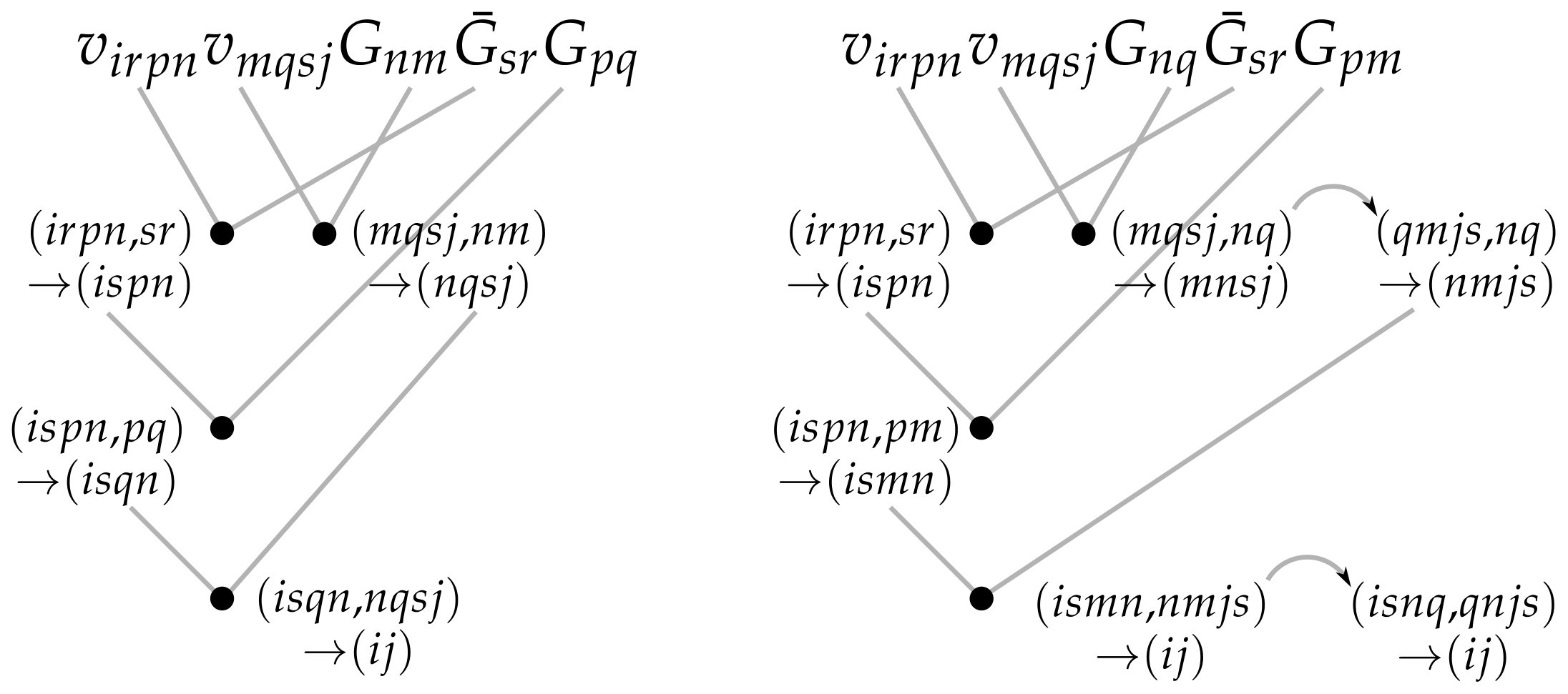 Figure 1
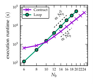 Figure 2
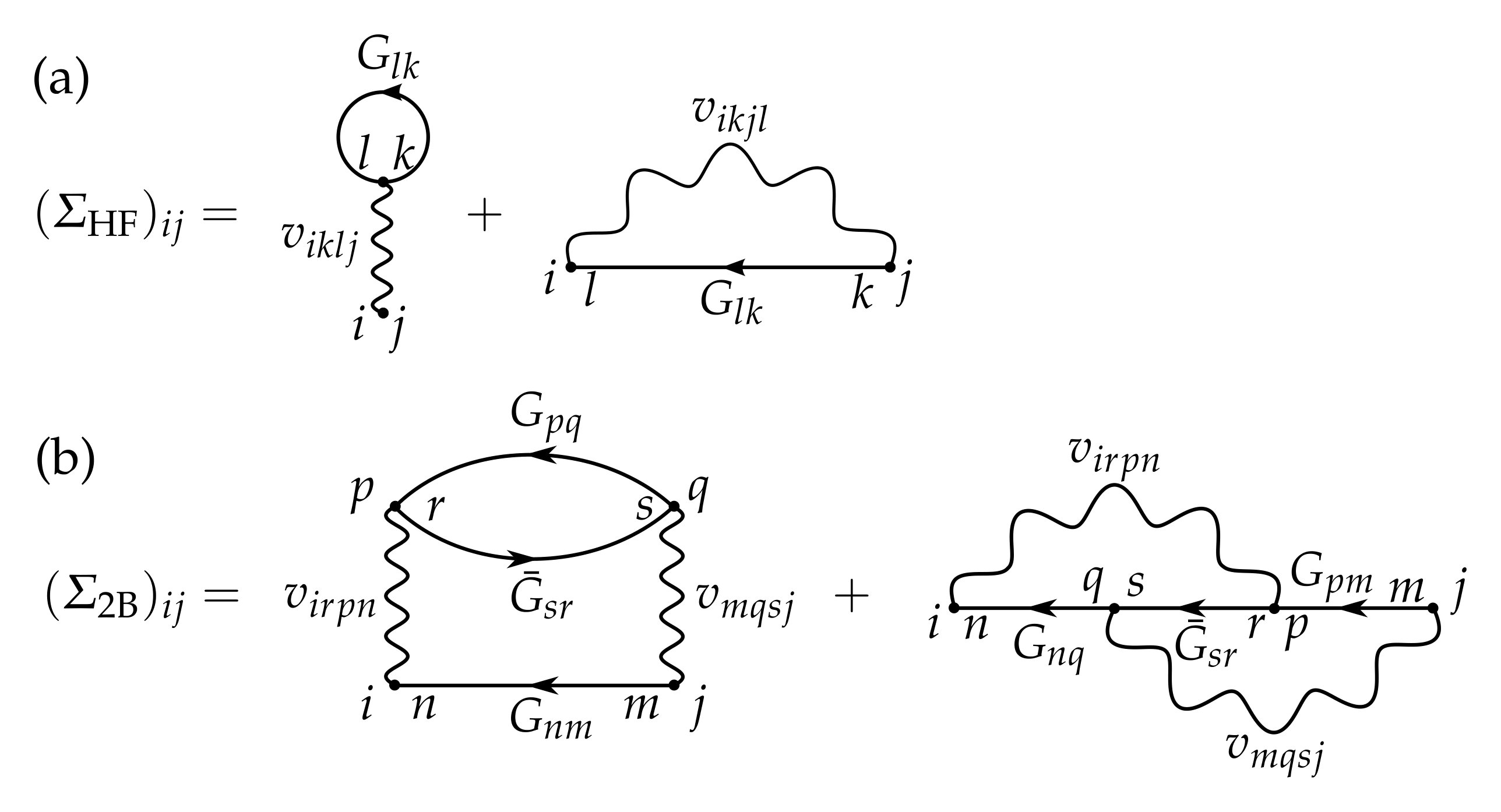 Figure 3
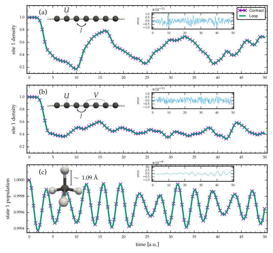 Figure 4
| Basis | Scaling | Time (loop) | Time (contr.) | Gain |
|---|---|---|---|---|
| diagonal | 177 | 164 | 1.08 | |
| symmetric | 1213 | 731 | 1.66 | |
| general | 1527 | 1333 | 1.15 |
Peer Reviews
No public reviews on file for this paper yet. If you reviewed it on a platform where reviews are public (OpenReview, ICLR, NeurIPS, ICML), you can paste yours below so the community can read it here.
Videos
No videos yet. Explain this paper in a talk, walkthrough, or lecture? Add one.
Efficient computation of the second-Born self-energy using tensor-contraction operations
Riku Tuovinen
Max Planck Institute for the Structure and Dynamics of Matter,
Luruper Chaussee 149, 22761 Hamburg, Germany
Fabio Covito
Max Planck Institute for the Structure and Dynamics of Matter,
Luruper Chaussee 149, 22761 Hamburg, Germany
Michael A. Sentef
Max Planck Institute for the Structure and Dynamics of Matter,
Luruper Chaussee 149, 22761 Hamburg, Germany
Abstract
In the nonequilibrium Green’s function approach, the approximation of the correlation self-energy at the second-Born level is of particular interest, since it allows for a maximal speed-up in computational scaling when used together with the Generalized Kadanoff-Baym Ansatz for the Green’s function. The present day numerical time-propagation algorithms for the Green’s function are able to tackle first principles simulations of atoms and molecules, but they are limited to relatively small systems due to unfavourable scaling of self-energy diagrams with respect to the basis size. We propose an efficient computation of the self-energy diagrams by using tensor-contraction operations to transform the internal summations into functions of external low-level linear algebra libraries. We discuss the achieved computational speed-up in transient electron dynamics in selected molecular systems.
pacs:
31.15.-p, 31.25.-v, 71.10.-w
I Introduction
A state-of-the-art computational method for out-of-equilibrium many-body physics is the nonequilibrium Green’s function (NEGF) approach Baym and Kadanoff (1961); Kadanoff and Baym (1962); Keldysh (1964); Danielewicz (1984a); Stefanucci and van Leeuwen (2013); Balzer and Bonitz (2013). Mostly due to lack of computational capabilities, the non-linear integro-differential Kadanoff-Baym equations (KBE) for the NEGF from the 1960s remained fairly elusive until their first numerical solutions were presented in 1984 by Danielewicz (1984b) and further numerical implementations at the turn of the century Köhler, Kwong, and Yousif (1999); Semkat, Kremp, and Bonitz (1999); Kwong and Bonitz (2000). During the past twenty years a considerable amount of progress has been achieved in various fields of physics employing the NEGF approach: From sub-atomic nuclear reactions Dickhoff and Barbieri (2004); Rios et al. (2011) to atomic and molecular scale Dahlen and van Leeuwen (2005, 2007); Galperin, Ratner, and Nitzan (2007); Thygesen (2008); Balzer, Bauch, and Bonitz (2010a, b); Phillips and Zgid (2014); Perfetto et al. (2015); Covito et al. (2018); Hopjan et al. (2018), further to condensed phase Freericks, Krishnamurthy, and Pruschke (2009); Moritz et al. (2013); Kemper et al. (2013); Sentef et al. (2013); Aoki et al. (2014); Kemper et al. (2014, 2015); Sentef et al. (2016); Golež, Werner, and Eckstein (2016); Kemper et al. (2017); Tuovinen et al. (2018) and mesoscopic systems Brandbyge et al. (2002); Ludovico and Arrachea (2012); Wang et al. (2014); Ridley and Tuovinen (2017); Tuovinen et al. (2019a, b), and even to descriptions of high-energy particle physics in cosmology Kainulainen et al. (2002); Garny and Müller (2009); Garny, Kartavtsev, and Hohenegger (2013).
However, combining the KBE with ab initio descriptions of realistic materials still remains a computational challenge. This challenge results from the double-time structure of the KBE rendering the method very expensive for both CPU time and storing the objects in RAM. The Generalized Kadanoff–Baym Ansatz (GKBA) offers a simplification by reducing the two-time-propagation of the Green’s function to the time-propagation of a time-local density matrix Lipavský, Špička, and Velický (1986). The computational complexity of the time-propagation of the GKBA equations scales as the number of time steps squared instead of the cubic scaling in the double-time KBE Hermanns, Balzer, and Bonitz (2012). When a simulation to reach longer time scales is desired, this difference in computational speed becomes immense. However, this speed-up in computational scaling is only possible for the correlation self-energy approximation at the second-Born (2B) level. The 2B approximation goes beyond mean-field description at the Hartree-Fock (HF) level but it includes the bare interaction only up to second order, i.e., higher order correlations and screening effects are neglected, like in higher order -matrix or approximations Galitskii (1958); Hedin (1965). However, the viability of the 2B approximation has been assessed for a large set of systems with up to moderate interaction strength von Friesen, Verdozzi, and Almbladh (2009); Rusakov and Zgid (2016).
Even though the above implementations of the NEGF method have been successfully applied in many contexts, the computation of the self-energy still remains a numerical bottleneck. For larger systems to be studied, the scaling with respect to the basis size in the self-energy diagrams may be very unfavourable, making first principles simulations numerically expensive, at least in naïve implementations when looping over the full basis. Recently, a dissection algorithm has been proposed and implemented Perfetto and Stefanucci (2019, 2018) for identifying and utilizing the sparsity of many-body interactions. In this paper we propose to transform the summation expressions in the self-energy diagrams using tensor-contraction operations, and to further employ external linear algebra libraries (e.g. low-level C or Fortran) taking into account, e.g., memory availability, communication costs, loop fusion and ordering Baumgartner et al. (2005); Solomonik et al. (2014); Huang, Matthews, and van de Geijn (2018). (Here we consider tensors simply as multidimensional objects without deeper (differential-)geometric interpretation.) With benchmark simulations in selected molecular systems we present an efficient way to compute the 2B self-energy applicable either in full time-propagation of the KBE or in the numerically less expensive GKBA variant.
II Model and method
We consider a finite and quantum-correlated electronic system described by a time-dependent Hamiltonian
[TABLE]
where label a complete set of one-particle states \{\varphi(\mbox{\boldmathr})\}, and are the annihilation (creation) operators for electrons from (to) these states. Although we assume, for simplicity, spin-compensated electrons and invariance under spin rotations, the whole consideration could easily be generalized to include also spin degrees of freedom Myöhänen et al. (2008, 2009); von Friesen, Verdozzi, and Almbladh (2009); Latini et al. (2014); Giesbertz (2016). The objects henceforth described will be diagonal in spin space. The one-body contribution to the Hamiltonian,
[TABLE]
may have an explicit time dependence, describing, e.g., pump-probe spectroscopies or voltage pulses. These would enter in h(\mbox{\boldmathr},t)=-\frac{1}{2}\nabla^{2}+w(\mbox{\boldmathr},t)-\mu as external fields . We also introduced the chemical potential and we absorbed it into the equilibrium description of the one-body part of the Hamiltonian. Atomic units, , are used throughout. The two-body part accounts for interactions between the electrons with the standard two-electron Coulomb integrals
[TABLE]
Even though the Coulomb interaction itself is instantaneous, in Eq. (1) we allow the strength of the two-body part to be time-dependent to describe, e.g., interaction quenches or adiabatic switching. For real-valued basis functions the Coulomb integrals in Eq. (3) follow -point permutation symmetry
[TABLE]
which can be verified by permuting dummy integration variables and by complex conjugation. The following discussion is not limited to this choice, however, and also complex and spin-dependent basis functions could be used.
To calculate time-dependent nonequilibrium quantities we use the equations of motion for the one-particle Green’s function on the Keldysh contour Danielewicz (1984a); Stefanucci and van Leeuwen (2013); Balzer and Bonitz (2013). This object is defined as
[TABLE]
where is the contour ordering operator and the variables specify the location of the Heisenberg-picture operators on the Keldysh contour. The contour has a forward and a backward branch on the real-time axis, , and also a vertical branch on the imaginary axis, with inverse temperature . The Green’s function includes detailed information about particle propagation, and important physical quantities such as electric currents or photoemission spectra can be extracted from it. The Green’s function satisfies the integro-differential equations of motion Stefanucci and van Leeuwen (2013)
[TABLE]
where all objects are matrices with respect to the basis of one-particle states \{\varphi(\mbox{\boldmathr})\}. The self-energy accounts for the electronic interactions. While some two-particle quantities, such as interaction energies and double occupancies, can also be computed from this picture Balzer (2011); Balzer, Schlünzen, and Bonitz (2016), the introduction of the self-energy transforms the many-body problem to an effective quasiparticle picture, and higher order correlations, such as the pair distribution function, are not directly accessible von Friesen, Verdozzi, and Almbladh (2011); Bonitz et al. (2013). Depending on the arguments , the Green’s function, , and the self-energy, , defined on the time contour have components lesser (), greater (), retarded (R), advanced (A), left (), right () and Matsubara (M) Stefanucci and van Leeuwen (2013). Typically, one concentrates on the particle and hole propagation in terms of and where the time arguments and refer to the (real) times when a particle is added or removed from the system. Furthermore, the one-particle reduced density matrix (1RDM) is from which one could compute the expectation value of any one-body operator. Taking the equal-time limit () one obtains from Eqs. (6) and (7)
[TABLE]
where we defined the collision integral
[TABLE]
In addition, in Eq. (8) we separated the time-local and time-non-local contributions to the self-energy as , the former being referred to as the Hartree-Fock (HF) self-energy and the latter the correlation self-energy, see Fig. 1. This allows for the extraction of a time-local effective single-particle Hamiltonian, . The collision integrals therefore incorporate only the correlation self-energies . Importantly, the self-energies depend on the Green’s functions themselves, , and therefore the equation of motion needs to be solved self-consistently. The correlation self-energies are typically obtained by a diagrammatic expansion where terms can be systematically summed up to infinite order. In this work we concentrate on the second-Born self-energy, , see Fig. 1, but the consideration can be extended to other (higher order) diagrams as well.
Although we reduced the considered information to the description of a single-time object , the double-time nature of the full equations of motion is still present in the collision integral which requires the double-time history of and to be stored. In order to obtain a closed equation for it is customary to use the GKBA Lipavský, Špička, and Velický (1986)
[TABLE]
and an approximation to the double-time propagators at the HF level Balzer and Bonitz (2013)
[TABLE]
where is the chronological time-ordering operator Stefanucci and van Leeuwen (2013). The HF self-energy, being time-local, can be evaluated from the 1RDM as (see Fig. 1)
[TABLE]
The lesser Green’s function or the 1RDM can then be solved from Eq. (8) by a numerical time-stepping algorithm and using the symmetry property Hermanns, Balzer, and Bonitz (2012); Latini et al. (2014); Tuovinen et al. (2018).
In principle, the collision integral on the vertical branch of the Keldysh contour, , should also be taken into consideration. However, using the GKBA, the initial correlations collision integral, , is usually neglected due to the lack of a GKBA-like expression for the mixed components and . The correlated initial state therefore needs to be prepared by starting with an uncorrelated (or HF) system and slowly switching on the interaction (adiabatic switching procedure) Hermanns, Balzer, and Bonitz (2012); Latini et al. (2014); Hermanns, Schlünzen, and Bonitz (2014); Tuovinen et al. (2018). However, the inclusion of the initial correlations has been shown to be possible also within GKBA Semkat, Bonitz, and Kremp (2003); Karlsson et al. (2018); Hopjan and Verdozzi (2019).
III Second-Born self-energy
For the time-propagation of Eq. (8) we are only concerned with the lesser and greater components of the Green’s function and self-energy. For the sake of notational simplicity, we then write , , and . In the second-Born approximation (2B) the correlation self-energy takes the form Latini et al. (2014); Perfetto and Stefanucci (2019) (see Fig. 1)
[TABLE]
As can be seen from Eq. (III) computing the full self-energy matrix by direct looping takes operations where is the size of the basis. However, it is possible to reduce this scaling to by grouping and reorganizing the objects in Eq. (III) Yang et al. (2011); Hermanns (2016); Neuhauser, Baer, and Zgid (2017); Karlsson et al. (2018); Perfetto and Stefanucci (2019); Schluenzen et al. (2019). We address this more thoroughly in Sec. III.3. It is also to be noted that the 2B self-energy is non-local in time, i.e., this computation needs to be performed for two times and , and it is important to keep track of the correct time arguments in the objects , and . While the 2B approximation together with the GKBA allows for a maximal speed-up in computational scaling compared to the full two-time KBE ( vs. , being the total propagation time), GKBA simulations with and -matrix approximations to the self-energy have also been performed Schlünzen and Bonitz (2016); Schlünzen et al. (2017).
We note that the NEGF method using the 2B self-energy, sometimes referred to as second-order Green’s function (GF2) Holleboom and Snijders (1990); Phillips and Zgid (2014); Rusakov and Zgid (2016); Neuhauser, Baer, and Zgid (2017), can be related to the second-order Møller-Plesset perturbative expansion (MP2) Helgaker, Jørgensen, and Olsen (2000). The construction of the MP2 correction is similar to the 2B self-energy, although in the NEGF approach the self-energy enters nonlinearly into an updated Green’s function and this procedure is continued until convergence is reached, whereas the MP2 can be related to the first step of this iteration Holleboom and Snijders (1990); Phillips, Kananenka, and Zgid (2015); Neuhauser, Baer, and Zgid (2017).
Next, we consider three different cases for the interaction vertex: (1) Diagonal basis where the Coulomb integrals take the Hubbard-like form ; (2) Symmetric basis where the Coulomb integrals allow for non-diagonal or long-range interactions but the -point vertex is symmetric (density-density type interaction); and (3) The general basis of the full Coulomb integral . From the resulting structures of the internal summations in the self-energy diagrams, we identify matrix or tensor operations. Instead of simply looping over the basis indices, employing well-established linear algebra libraries for the matrix and tensor operations Baumgartner et al. (2005); Solomonik et al. (2014); Huang, Matthews, and van de Geijn (2018) may speed up the construction of the self-energy.
We denote matrix multiplication by “” and entrywise multiplication (Hadamard or Schur product) by “”. For example, in Fortran and Mathematica the entrywise products are done through simple multiplication operator “” whereas the matrix product is done through the “matmul” or “.” operators. In C++ with the Armadillo library Sanderson and Curtin (2016) the symbol “%” is used for entrywise products whereas “” is a matrix product. In Python with the NumPy (np) numerical library Oliphant (2006) the entrywise product can be done with the function “np.multiply” whereas the matrix or more general tensor multiplication can be done via the “np.dot” or the “np.einsum” functions.
III.1 Diagonal basis
For a diagonal basis, , Eq. (III) is simplified as
[TABLE]
and the computational cost of constructing the full matrix therefore scales as . In this simple case there are no further contractions to perform as the internal summations were already explicitly resolved due to the Kronecker ’s in the interaction vertex. Because in many practical implementations entrywise multiplication between two objects is only possible when they have the same dimension, we rewrite the on-site interaction instead as the diagonal part of a matrix. The resulting expression can then be recasted in matrix form as an entrywise product
[TABLE]
We anticipate that this is a faster construction for the whole self-energy matrix instead of looping over the basis indices in Eq. (14) when passing the matrix operations in Eq. (15) to an external linear algebra library.
III.2 Symmetric basis
For a symmetric basis, , Eq. (III) is simplified as
[TABLE]
We first consider the first term of Eq. (16), i.e., the second-order bubble diagram, and visualize the contraction path for efficient computation. The expression can be manipulated as
[TABLE]
where we identified matrix transposes, entrywise products and matrix multiplications. The procedure outlined above, unfortunately, makes the final expressions less readable, but in the end the full self-energy matrix (for the bubble diagram part) may be constructed as a one-liner . However, as mentioned earlier, one must keep track of the time arguments, i.e., reading from left the first is evaluated at and the second is evaluated at .
Contractions on the internal summations in the self-energy diagrams do not always yield a favourable path. If we take the second term in Eq. (16), i.e., the second-order exchange diagram, obtaining an expression similar to Eq. (17) is not possible for the full self-eneregy matrix. However, for the diagonal part of the exchange diagram we obtain
[TABLE]
The off-diagonal parts would still need to be evaluated by explicit looping as in Eq. (16), but the above contraction path may also be combined with, e.g., the dissection algorithm of Ref. Perfetto and Stefanucci (2019) where chosen pairs of the Coulomb integral matrix elements (according to some cut-off energy) would be used. This further reduces the requirement for looping over the basis indices.
III.3 General basis
For a general basis all are nonvanishing. In this case the multi-index summations in the self-energy diagrams and their consequent contractions are not always easy to see, but this task can be automatized using, e.g., the np.einsum_path function in Python. The information obtained for an optimal sequence of contractions may further be combined with the symmetry properties (4) and with a pre-determined subset of nonzero Coulomb integrals Perfetto and Stefanucci (2019).
Manipulating Eq. (III) gives
[TABLE]
where we defined tensor contractions and permuted indices with the help of Eq. (4), identifying similar contractions consequently. We see from the last line of Eq. (III.3) that for constructing the full self-energy matrix the scaling over the basis is reduced from to Hermanns (2016); Neuhauser, Baer, and Zgid (2017); Perfetto and Stefanucci (2019); Schluenzen et al. (2019).
As before, the readability of the self-energy in Eq. III.3 suffers a bit compared to Fig. 1 or Eq. (III). However, Eq. (III.3) is visualized in Fig. 2, and for the sake of efficient computation the contraction operations can be grouped together and executed essentially as a single command, where the lower-level loop fusions and orderings of operations are handled by the underlying numerical library. We emphasize that while the reorganizations of the summations in Eq. (III) to arrive at Eq. (III.3) have already been considered to some degree in Refs. Hermanns (2016); Perfetto and Stefanucci (2019); Schluenzen et al. (2019), here we concentrate on the practical computation of the self-energy by employing efficient tensor-contraction operations with a possible contraction path shown in Fig. 2. Alternative contraction paths than the one shown in Fig. 2 are also possible.
IV Numerical benchmarks
For the three different cases presented in the previous section, (1) diagonal, (2) symmetric and (3) general bases, we now present sample numerical simulations for the purpose of benchmarking and assessing the validity and accuracy of the alternative implementations of the 2B self-energy. For test cases we choose molecular systems falling into each of the categories: D Hubbard chains which can be related to, e.g., conjugated polymers Kirtman and Champagne (1997); van Faassen et al. (2002, 2003); Hermanns, Schlünzen, and Bonitz (2014) with local (1) and long-range interactions (2). We set the hopping energy between nearest-neighbors , the on-site electron-electron interaction , and the long-range interaction between particles at atomic sites and as in the Ohno model Ohno (1964); Baeriswyl, Campbell, and Mazumdar (1992). For the case (3) we take a molecule with a general one-particle Kohn-Sham (KS) basis obtained from density-functional theory (DFT) using Octopus Marques et al. (2003). Using this DFT calculation, the one- and two-body matrix elements [Eqs. (2) and (3)] are then constructed in the corresponding KS basis; a more detailed explanation can be found in Ref. Perfetto and Stefanucci (2018).
We implement the explicit loops over the basis indices [Eqs. (14), (16), and (III.3)] in C++. In the cases (1) and (2) we employ the matrix operations [Eqs. (15), (17), and (18)] using the Armadillo library (version 9.200.5) Sanderson and Curtin (2016), and in the case (3) we employ the tensor operations [Eq. (III.3) and Fig. 2] using the NumPy library (version 1.15.1) in Python Oliphant (2006). We perform the comparisons using a regular desktop computer with an Intel Core i5-4460 @ 3.2 GHz with 6 MB cache, running on 64-bit architecture using Ubuntu 18.04 operating system incorporating the Linux kernel 4.15.0 and the GCC 7.3.0 compiler. The comparisons are done using only a single core to better benchmark the computational cost.
We perform a time-propagation à la GKBA of time steps with length . For the sake of simpler computation, in this work we do not employ any predictor-corrector schemes. For the polymer chain we take atomic sites and start the time-propagation from an initial state where particles are trapped to the leftmost sites by applying a strong confinement potential Hermanns, Schlünzen, and Bonitz (2014). This configuration relaxes once the time evolution is started. For the molecule we represent the electrons by basis functions, and we start the time-propagation from a HF initial state, which can be obtained from a separate (time-independent) calculation, and then suddenly switch on the many-body correlations in the 2B self-energy. This sudden process can be interpreted as an interaction quench introducing transient dynamics.
For the case (1) we take time steps of length , for the case (2) time steps of length , and for the case (3) we take time steps of length . The reason for the varying number of time steps between the investigated cases is that a calculation with would be too fast to execute in case (1) for a meaningful comparison of runtimes, whereas in case (3) would lead to unpractically long execution times for the sake of the present study. Here we are not too concerned about the physical mechanisms taking place during the transient oscillations or how accurate the 2B self-energy is compared to more sophisticated approximations, but our aim is simply to assess the validity of the proposed computation scheme, and to compare execution runtimes.
In Fig. 3 we show the transient dynamics of the three cases discussed above. The execution runtimes for each of these simulations are shown in Tab. 1. We confirm that within numerical accuracy, both looping over the basis indices and employing tensor-contraction operations, give the same result. Importantly, the execution runtimes are brought down by employing the tensor-contraction operations in the computation of the 2B self-energy. Furthermore, we have checked by increasing the number of time steps that the runtimes increase accordingly, i.e., the gain factors in Tab. 1 remain roughly similar. For additional validation we have compared our data in Fig. 3(c) against the CHEERS code Perfetto and Stefanucci (2018) and we find perfect agreement. We note in passing that an ill-advised looping over the full basis in Eq. (III) () instead of the reduced looping in Eq. (III.3) () would result in considerably higher execution runtimes.
As the number of basis functions was relatively small in the previous calculations, we expect increase in the gain factors when larger basis is used, due to profiting more from the optimized underlying numerical libraries. In Fig. 4 we show the execution runtimes corresponding to Fig. 3(c) but with varying number of basis functions. With explicit looping over the basis indices we observe behaviour. For smaller basis sizes the explicit looping is faster compared to the tensor-contraction operations done on the NumPy arrays. However, for larger basis sizes the runtimes using the tensor-contraction operations are significantly smaller, also following a power law behaviour for which we empirically find , see Fig. 4. This exponent and its statistical errors were extracted by performing a nonlinear least squares fit to the flat part, , using gnuplot. This reduced scaling could be related to the optimization of matrix multiplication using the Strassen algorithm Strassen (1969), and to more advanced methods for tensor contraction algorithms which can scale faster than the naïve looping scheme Huang, Matthews, and van de Geijn (2018).
V Conclusion
We presented an efficient way to compute the 2B self-energy diagrams, in the NEGF approach, by using tensor-contraction operations. The apparent attraction for efficient computation of the 2B self-energy, in particular, was due to the maximal speed-up in computational scaling when used together with the GKBA. The internal summations in the self-energy calculations were transformed into matrix and tensor operations to be performed by external low-level linear algebra libraries, speeding up the computation. We anticipate the speedup may be even more advantageous when the code is executed in parallel, taking full advantage of the optimized underlying numerical libraries. Instead of looping over the basis indices, utilizing efficiently optimized external numerical libraries for the tensor-contraction operations has the further advantage of speeding up the computation if/when future implementations of the the external libraries become faster and even more efficient Huang, Matthews, and van de Geijn (2018).
There has been recent progress in reducing the computational bottleneck of constructing various self-energy approximations by using stochastic methods Ge et al. (2014); Neuhauser et al. (2014); Neuhauser, Baer, and Zgid (2017). Here we mention the work of Neuhauser, Baer, and Zgid (2017) who considered the 2B self-energy in an equilibrium setting and achieved a much more favourable quadratic scaling over the fifth power. While the reduced scaling with respect to the basis size using these stochastic methods goes beyond our findings, it is not straightforward to argue how the accuracy of such a stochastic-sampling approach may affect convergence or error propagation in an out-of-equilibrium setting. In this case one would have to sample not a single -axis (Matsubara) self-energy but instead a new slice of ever-expanding self-energies in the two-time plane. However, it would be a promising venue to extend the stochastic methods also to real time in future studies Ruan and Baer (2018).
The presented approach is not limited to the 2B self-energy only but could be readily used for other correlation self-energies, such as or -matrix. In addition, many other similar multi-index operations, such as evaluating the initial correlations collision integral in Ref. Karlsson et al. (2018), might become computationally more accessible by using the tensor-contraction representations. In the present work we considered only the GKBA with Hartree-Fock propagators, but extensions to correlated approximations to the propagator Latini et al. (2014) are also directly applicable in our approach. The presented simulations in selected molecular systems provided concrete evidence of the accuracy and applicability of the tensor-contraction operations. With reasonable and precise implementations or variations of the present study, we expect this procedure to allow for considerably larger basis sizes to be possible to address in forthcoming NEGF+first principles simulations.
Acknowledgements.
R.T. and M.A.S. acknowledge funding by the DFG (Grant No. SE 2558/2-1) through the Emmy Noether program. We wish to thank Damian Hofmann, Gianluca Stefanucci, Michael Bonitz, and Angel Rubio for productive discussions.
The reference list from the paper itself. Each links out to its DOI / PubMed record.
- 1Baym and Kadanoff (1961) G. Baym and L. P. Kadanoff, Phys. Rev. 124 , 287 (1961) . · doi ↗
- 2Kadanoff and Baym (1962) L. P. Kadanoff and G. Baym, Quantum Statistical Mechanics (W. A. Benjamin, New York, 1962).
- 3Keldysh (1964) L. V. Keldysh, Zh. Eksp. Teor. Fiz. 47 , 1515 (1964), [Sov. Phys. JETP 20 , 1018 (1965)].
- 4Danielewicz (1984 a) P. Danielewicz, Ann. Phys. (N. Y.) 152 , 239 (1984 a) . · doi ↗
- 5Stefanucci and van Leeuwen (2013) G. Stefanucci and R. van Leeuwen, Nonequilibrium Many-Body Theory of Quantum systems: A Modern Introduction (Cambridge University Press, Cambridge, 2013).
- 6Balzer and Bonitz (2013) K. Balzer and M. Bonitz, Nonequilibrium Green’s Functions Approach to Inhomogeneous Systems (Springer Berlin Heidelberg, 2013). · doi ↗
- 7Danielewicz (1984 b) P. Danielewicz, Ann. Phys. (N. Y.) 152 , 305 (1984 b) . · doi ↗
- 8Köhler, Kwong, and Yousif (1999) H. S. Köhler, N. H. Kwong, and H. A. Yousif, Comp. Phys. Commun. 123 , 123 (1999) . · doi ↗