Odd-frequency superconducting pairing in Kitaev-based junctions
Athanasios Tsintzis, Annica M. Black-Schaffer, Jorge Cayao

TL;DR
This paper explores odd-frequency superconducting correlations in Kitaev chain-based junctions, revealing how Andreev reflections and Majorana modes influence pairing amplitudes and local density of states in topological phases.
Contribution
It demonstrates the role of Andreev reflections in odd-frequency pairing and characterizes Majorana-induced features in local states within Kitaev-based superconducting junctions.
Findings
Odd-frequency pairing is enhanced at interfaces in the topological phase.
Majorana zero modes cause a resonance peak in odd-frequency amplitude at phase difference π.
Both even- and odd-frequency pairings reveal topological Andreev bound states.
Abstract
We investigate odd-frequency superconducting correlations in normal-superconductor (NS) and short superconductor-normal-superconductor (SNS) junctions with the S region described by the Kitaev model of spinless fermions in one dimension. We demonstrate that, in both the trivial and topological phases, Andreev reflection is responsible for the coexistence of even- and odd-frequency pair amplitudes at interfaces, while normal reflections solely contribute to odd-frequency pairing. At NS interfaces we find that the odd-frequency pair amplitude exhibits large, but finite, values in the topological phase at low frequencies. This enhancement is due to the emergence of a Majorana zero mode at the interface, but notably there is no divergence and a finite odd-frequency pair amplitude also exists outside the topological phase. We also show that the local density of states and local odd-frequency…
Click any figure to enlarge with its caption.
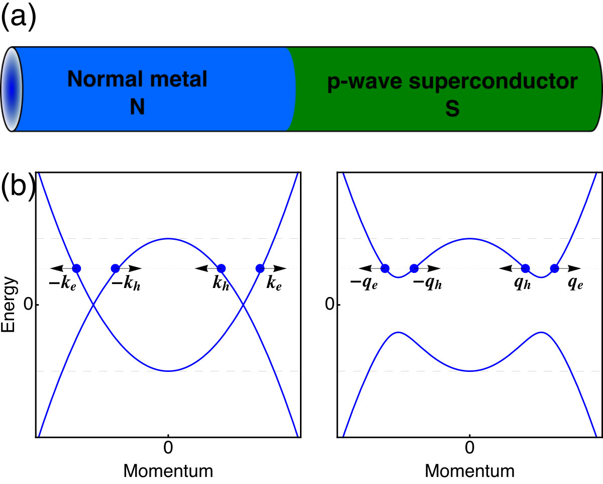 Figure 0
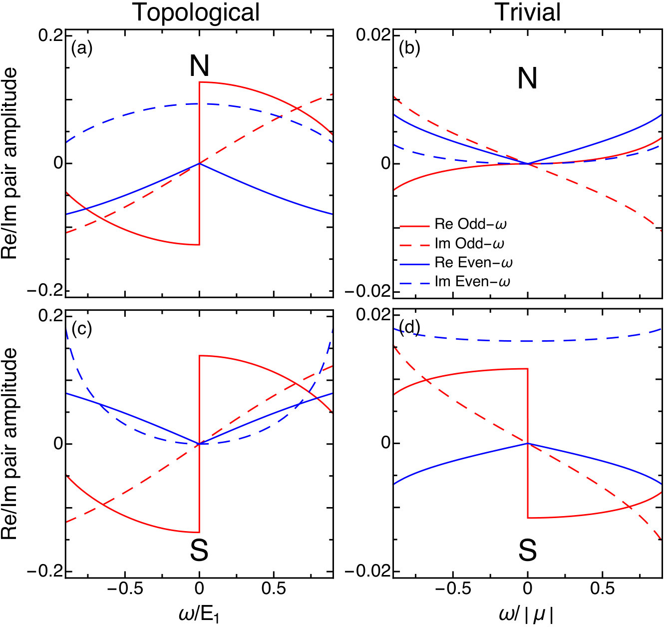 Figure 1
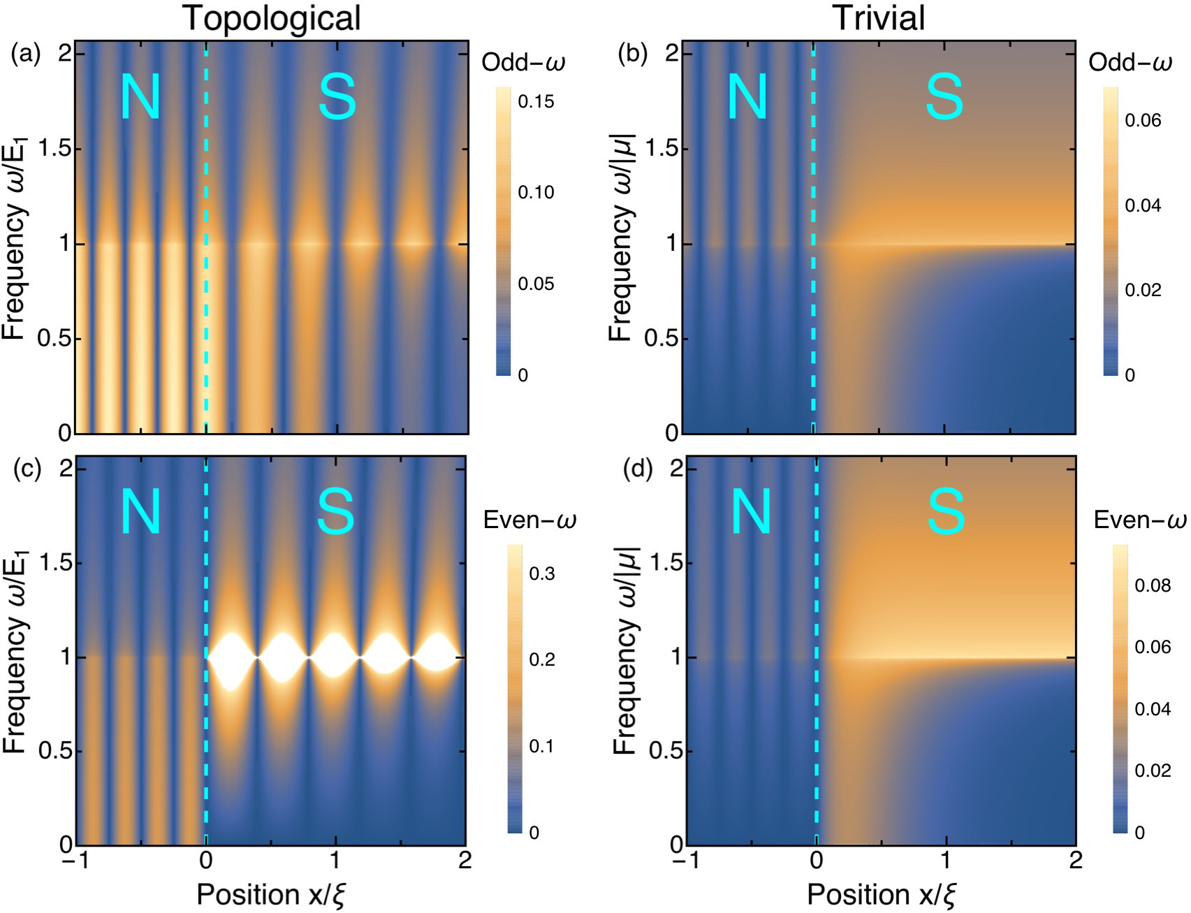 Figure 2
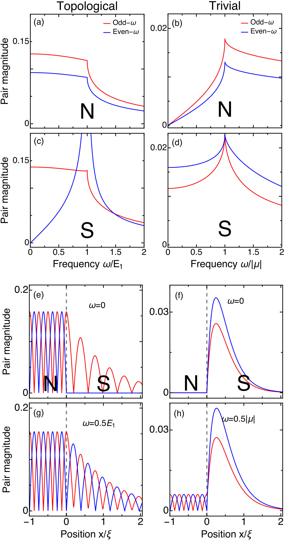 Figure 3
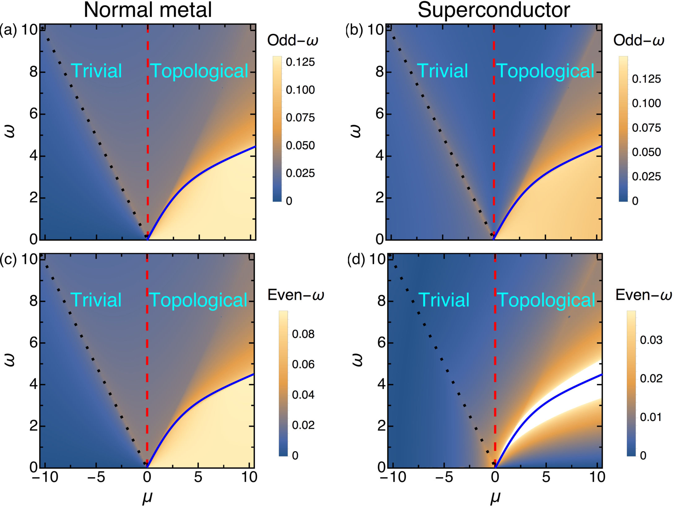 Figure 4
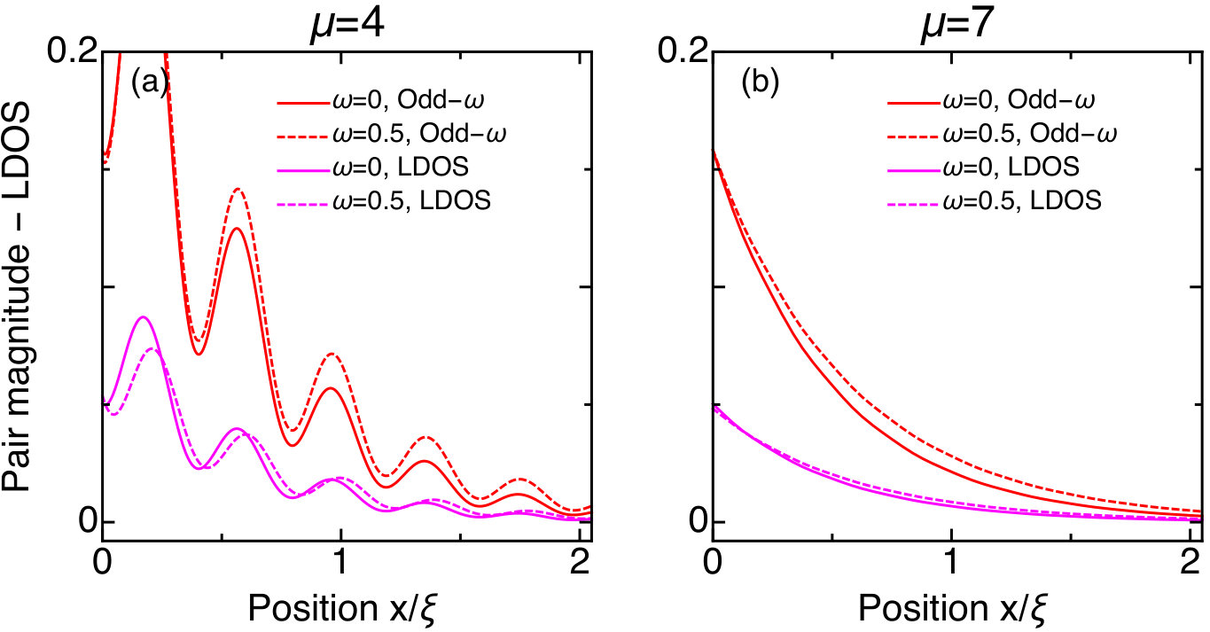 Figure 5
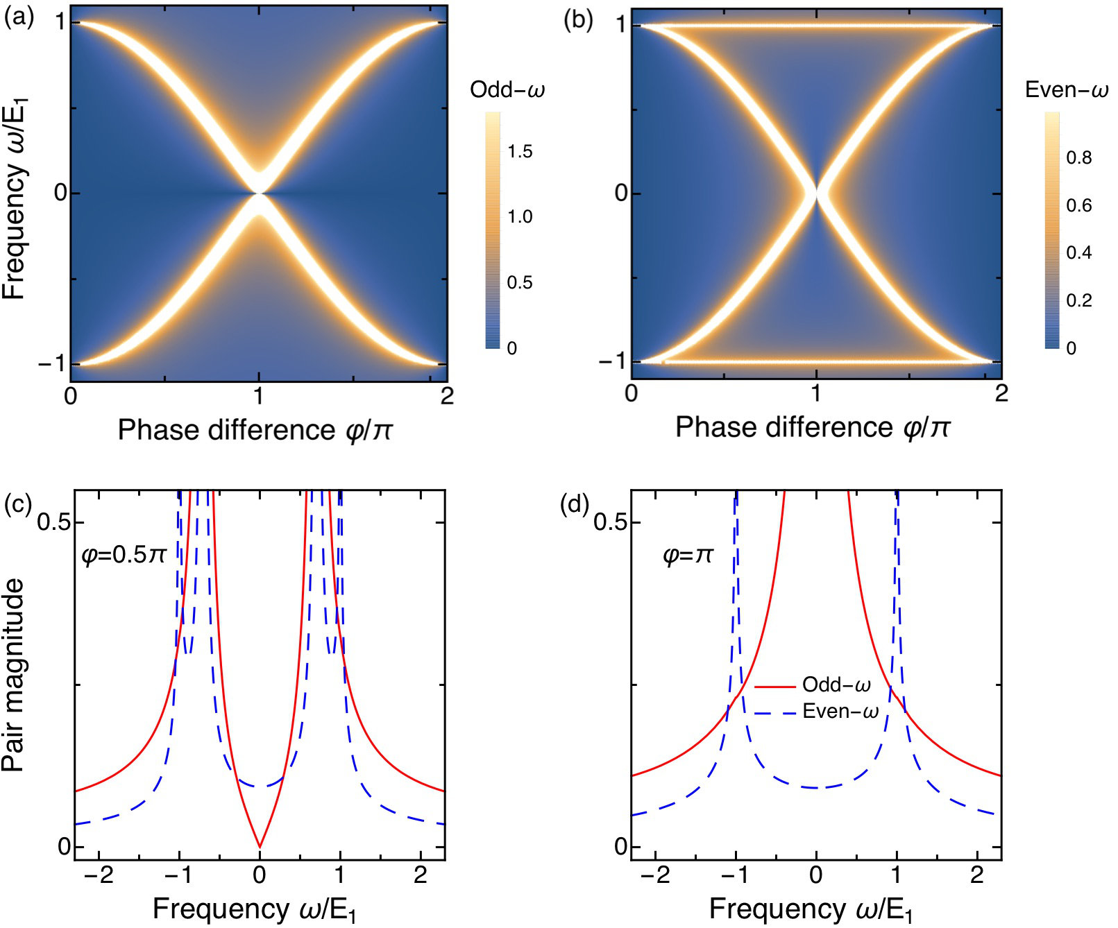 Figure 6
| , | ||
Peer Reviews
No public reviews on file for this paper yet. If you reviewed it on a platform where reviews are public (OpenReview, ICLR, NeurIPS, ICML), you can paste yours below so the community can read it here.
Videos
No videos yet. Explain this paper in a talk, walkthrough, or lecture? Add one.
Odd-frequency superconducting pairing in Kitaev-based junctions
Athanasios Tsintzis
Department of Physics and Astronomy, Uppsala University, Box 516, S-751 20 Uppsala, Sweden
Division of Solid State Physics and NanoLund, Lund University, Box 118, S-221 00 Lund, Sweden
Annica M. Black-Schaffer
Jorge Cayao
Department of Physics and Astronomy, Uppsala University, Box 516, S-751 20 Uppsala, Sweden
Abstract
We investigate odd-frequency superconducting correlations in normal-superconductor (NS) and short superconductor-normal-superconductor (SNS) junctions with the S region described by the Kitaev model of spinless fermions in one dimension. We demonstrate that, in both the trivial and topological phases, Andreev reflection is responsible for the coexistence of even- and odd-frequency pair amplitudes in N and S close to the interfaces, while normal reflections additionally only contributes to odd-frequency pairing in S. In the S region close to the NS interface we find that the odd-frequency pair amplitude exhibits large, but finite, values in the topological phase at low frequencies due to the emergence of a Majorana zero mode at the interface which also spreads into the N region. We also show that in S both the local density of states and local odd-frequency pairing can be characterized solely by Andreev reflections deep in the topological phase. Moreover, in the topological phase of short SNS junctions, we find that both even- and odd-frequency amplitudes capture the emergence of topological Andreev bound states. For a superconducting phase difference the odd-frequency magnitude exhibits a linear frequency () dependence at low-frequencies, while at it develops a resonance peak () due to the protected Majorana zero modes.
I Introduction
The properties of a superconductor are to a very high degree given by the symmetries of the electron pair amplitude. Due to Fermi-Dirac statistics, the pair amplitude is necessarily antisymmetric under the total exchange of all quantum numbers. In the simplest situation, these degrees of freedom include time (or frequency), spin, and spatial coordinates. Conventionally, electron pairing occurs between electrons at equal times, leading to pairing with even-frequency, spin-singlet, and even parity (e.g. the conventional superconducting state) or even-frequency, spin-triplet, and odd parity symmetries. However, in its more general form, pairing can occur at different times and also be odd in the relative time, or equivalently frequency, coordinate, enabling the possibility of odd-frequency superconducting pairing, such as odd-frequency, spin-singlet, and odd-parity or odd-frequency, spin-triplet, and even parity symmetries.
Odd-frequency pairing was initially considered as an intrinsic phenomenon in superfluid Helium Berezinskii (1974) and later investigated for superconductivity.Kirkpatrick and Belitz (1991); Balatsky and Abrahams (1992); Belitz and Kirkpatrick (1992); Balatsky and Bonča (1993); Abrahams et al. (1995); Coleman et al. (1997); Belitz and Kirkpatrick (1999) This exotic pairing can also arise as an intrinsic effect in multiband superconductorsBlack-Schaffer and Balatsky (2013a); Komendová et al. (2015); Asano and Sasaki (2015); Komendová and Black-Schaffer (2017); Triola and Black-Schaffer (2018) or it can be induced in superconducting hybrids or junctions,Bergeret et al. (2001); Tanaka and Golubov (2007); Tanaka et al. (2007a); Eschrig et al. (2007); Yokoyama et al. (2007); Tanaka et al. (2007b, 2012); Black-Schaffer and Balatsky (2012); Asano and Tanaka (2013); Black-Schaffer and Balatsky (2013b); Alidoust et al. (2015); Huang et al. (2015); Burset et al. (2015); Crépin et al. (2015); Reeg and Maslov (2015); Ebisu et al. (2016); Bobkova and Bobkov (2017); Hwang et al. (2018); Burset et al. (2017); Lu and Tanaka (2018); Cayao and Black-Schaffer (2017); Kuzmanovski and Black-Schaffer (2017); Keidel et al. (2018); Fleckenstein et al. (2018a); Balatsky et al. (2018); Breunig et al. (2018); Cayao and Black-Schaffer (2018); Tamura and Tanaka (2019) as well as under time-dependent fields.Triola and Balatsky (2016, 2017)
A large part of the relevance of odd-frequency pairing comes from allowing for highly unconventional superconducting correlations. For example, experiments have demonstrated that odd-frequency pairing enables a long-range proximity effect in ferromagnet-superconductor junctions.Petrashov et al. (1994); Bernardo et al. (2015) In this case, the ferromagnet induces a spin-singlet to triplet conversion while still keeping the robust -wave spatial parity, thus allowing superconductivity to survive and propagate in the ferromagnet. Similarly, in non-magnetic junctions, odd-frequency pairing is generated due to spatial parity breaking at the interface, which allows the conversion from -wave to -wave symmetry, while conserving the spin-singlet structure.Tanaka et al. (2007b) For a recent review on progress on odd-frequency superconductivity, see Ref. Linder and Balatsky, 2017.
Moreover, zero bias peaks have been reported in conductance measurements on many unconventional superconductors.Buchholtz and Zwicknagl (1981); Hara and Nagai (1986); Hu (1994); Tanaka and Kashiwaya (1995, 1996, 1997); Kashiwaya and Tanaka (2000) In some cases, such peaks correspond to the emergence of Majorana zero modes (MZMs) that signal a topological superconducting phase.Ryu and Hatsugai (2002); Kitaev (2001); Lutchyn et al. (2010); Oreg et al. (2010); Sato et al. (2011); Tanaka et al. (2012); Aguado (2017); Lutchyn et al. (2018) The MZM is a particle equal to its antiparticle and has attracted a great deal of attention due to its potential application in fault tolerant quantum computation.Kitaev (2001); Nayak et al. (2008); Sarma et al. (2015); Hwang et al. (2018); Schrade and Fu (2018) It has been shown that the frequency behavior of the pair amplitude produced by MZMs is highly unusual in the sense that it always exhibits an odd-frequency dependence.Asano and Tanaka (2013) This result is supported by further studies based on a quasiclassical approach in for example junctions with diffusive N regions,Tanaka and Golubov (2007); Tanaka et al. (2007b); Takagi et al. (2018) junctions with magnetic fields,Asano and Tanaka (2013) and systems deep in the topological phase with solely MZMs.Liu et al. (2015); Kashuba et al. (2017); Lee et al. (2017); Cayao and Black-Schaffer (2017); Tamura et al. (2019)
The fact that MZMs automatically give rise to odd-frequency pairing has raised the notion that these two concepts are intimately intertwined. On the other hand, MZMs only appear at boundaries of topological systems, and at boundaries there can also be odd-frequency pairing appearing simply due to spatial parity breaking. It is therefore natural to ask the question what is the relationship between MZMs and the associated topological phase, and odd-frequency pairing?. A detailed answer to this question is clearly important towards forming a more complete understanding of both odd-frequency pairing and MZMs.
The simplest platform in which to investigate MZMs is the Kitaev model,Kitaev (2001) which describes a one-dimensional -wave superconducting wire with spinless or spin-polarized fermions. This model exhibits a topological superconducting phase that is characterized by the emergence of MZMs in finite systems, one at each end of the wire, with their wavefunctions exponentially decaying into the bulk of the superconductor.Kitaev (2001) Despite its simplicity, the Kitaev model holds experimental relevance as its physical properties can be engineered by combining semiconducting nanowires with Rashba spin-orbit coupling and proximity-induced conventional -wave superconductivity, where an external magnetic field drives the system into its topological phase.Lutchyn et al. (2010); Oreg et al. (2010) This extension of the Kitaev model has led to great experimental activity with remarkable results during the past few years.Chang et al. (2015); Higginbotham et al. (2015); Krogstrup et al. (2015); Zhang et al. (2017); Albrecht et al. (2016); Deng et al. (2016); Nichele et al. (2017); Suominen et al. (2017); Chen et al. (2017); Deng et al. (2018); Zhang et al. (2018) Junctions based on the Kitaev model, therefore, represents both the simplest and the most natural platform for analyzing MZMs and their relation to odd-frequency pairing.
In this work we study NS and short SNS Kitaev-based junctions by employing a fully analytical quantum mechanical Green’s function approach to investigate the presence of odd-frequency pairing and its relation to MZMs. On one hand, NS junctions allow for the simplest study of interface scattering processes, including Andreev reflections, and thus allow for establishing their detailed relation to odd-frequency pairing and the emergence of a single MZM at the interface. On the other hand, short SNS junctions host a single pair of Andreev bound states (ABSs) in the energy gap at finite phase difference . These ABSs develop a protected zero energy crossing at in the topological phase which reflects the formation of a MZM pair, thus offering a clean way to study MZMs and odd-frequency pairing without the influence of any additional energy levels.
In general, we demonstrate that even- and odd-frequency pair amplitudes in the N and S regions coexist in both the trivial and topological phases due to Andreev reflections, which act as spatial parity mixers at interfaces. Normal reflections, however, solely contribute to odd-frequency pairing in the S regions, in contrast to junctions with conventional -wave superconductors.Burset et al. (2015); Cayao and Black-Schaffer (2018) For NS junctions in the topological phase, odd-frequency pairing in S is maximized around zero frequency due to the emergence of a MZM at the interface. However, it does not exhibit the dependence associated with an isolated MZM.Lee et al. (2017); Takagi et al. (2018); Tamura et al. (2019) Moreover, we also find that deep in the topological phase in S, Andreev reflection offers a simultaneous characterization of LDOS, conductance, and local odd-frequency pairing at the interface. Large values of LDOS or conductance in the low frequency topological regime therefore signify dominant odd-frequency correlations in S.
In short SNS junctions we show that both odd- and even-frequency amplitudes reveal the emergence of the topological ABSs at the junction. Interestingly, we obtain for an odd-frequency magnitude with a linear frequency () dependence at low-frequencies. At , however, the magnitude develops a resonance peak , revealing the MZM pair, which emerges due to the protected zero-frequency crossing at in this topological junction. The observation of a zero-frequency resonance peak in the LDOS at at the junction thus clearly indicates the presence of large odd-frequency correlations. This also applies to the -fractional Josephson effect as it occurs due to the protected zero frequency crossing at .Tanaka and Kashiwaya (1996); Kitaev (2001); Kwon et al. (2004)
We thus conclude that odd-frequency pairing is not restricted to either the topological phase and its MZMs, but appears very generally also in the absence of MZMs. The appearance of MZMs does enhance the odd-frequency pairing, but notably does not always appear as a sharp peak, instead giving a much more subtle contribution at NS interfaces.
The remainder of this article is organized as follows. In Sec. II we present the model and outline the employed method. In Sec. III we present our results for NS junctions in the trivial and topological phases. We then, in the same section, study the pair amplitudes in SNS junctions in the topological phase. Finally, we present our conclusions in Sec. IV. For completeness, we provide all the details on the derivation of the analytical calculations reported in this work in Appendices A-C.
II Model
The purpose of this work is to investigate the induced superconducting pair correlations in one-dimensional (1D) NS and short SNS junctions described by the 1D Kitaev model. As an example, a NS junction is schematically shown in Fig. 1(a), with the continuum Bogoliubov-de Gennes (BdG) Hamiltonian given by
[TABLE]
Here is the kinetic term set by the effective mass and momentum ,
with being the chemical potential in the normal (superconductor) region measuring the filling of the band, the strength of the interface barrier potential which controls the interface transparency, and the -wave pairing potential111Spatial variations of at the NS interfacesFleckenstein et al. (2018b) do not alter the main conclusions of this work. intrinsic to the Kitaev model with zero superconducting phase assumed for simplicity. Note that the N region is here spin-polarized or spinless, a property shared with the Kitaev model and also expected for a strong magnetic field applied along the wire needed to reach the topological phase in the S region. In what follows we use for simplicity of notation. The short SNS junction has a similar setup but with an additional S region with a superconducting phase difference between the two superconductors, and with the length of the normal part vanishing .
Diagonalizing the Hamiltonian in Eq. (1) in the normal state, , gives the eigenvalues plotted in Fig. 1(b) with wavevectors
[TABLE]
where . These wavevectors characterize the right and left moving electrons (holes) indicated by filled blue circles with horizontal arrows in Fig. 1(b). For the normal bands correspond to two parabolas that cross at and describe a metallic N region, while for the N region describes an insulator.
On the other hand, a finite opens a gap in the spectrum. The Kitaev model is particularly interesting because it realizes a topological phase with a MZM at each end of the wire.Kitaev (2001) It has been shown that at the spectrum of the -wave superconductor becomes gapless and signals the topological transition point between the trivial () and topological () phases. The gap of the spectrum is for and for , while in the trivial phase, , the gap is . The right panel of Fig. 1(b) shows the gapped spectrum in the topological phase, where it opens at the Fermi points . The wavevectors at finite are given by
[TABLE]
These wavevectors characterize the right and left moving quasielectrons (quasiholes) indicated by filled blue circles with horizontal arrows in right panel of Fig. 1(b). Moreover, can become complex valued depending of the values of , and , as discussed when necessary. Here, the superconducting coherence length is given by , where and , which reduces to for .
III Pair amplitude analysis
In order to capture odd-frequency pairing we need to analyze the superconducting pair amplitudes, which can be calculated from the anomalous electron-hole Green’s functions components. To this end, we first construct the retarded Green’s functions with outgoing boundary conditions in each region derived from the scattering processes at the interface.McMillan (1968) We here follow the approach developed in Refs. Cayao and Black-Schaffer, 2017, 2018, but for a comprehensive treatment, we provide the details in Appendix A. Note that this method is particularly suitable in this study because it both gives analytical access to the pair amplitudes and provides the scattering processes at the interfaces which hold experimental relevance in conductance measurements. Since the full derivations of the Green’s functions are straightforward but tedious we give them in Appendices B and C, for the NS and SNS systems, respectively.
With spin not being explicitly present in the system, is a matrix in electron-hole space, whose off-diagonal element directly gives the pair amplitudes
[TABLE]
Note that the spin-symmetry of the pair amplitude corresponds to the spin configuration in the Kitaev model, where the spinless consideration has to be understood in terms of a single spin species or a spin-polarized texture. Therefore, the spin-symmetry of Eq. (4) automatically corresponds to the equal spin-triplet component ( or ). The even and odd-frequency components of the pair amplitude are obtained from
[TABLE]
where corresponds to the advanced pair amplitude and is found using Eq. (4) from the relation . Here we have used that when considering negative frequencies () the advanced functions must be used instead of the retarded function.Cayao and Black-Schaffer (2017) Note also that Eq. (5) is valid for , so if plotting results for we have to instead use the advanced counterparts. This is a standard procedure when working with retarded and advanced Green’s functions, as for example described in Ref. Linder and Balatsky, 2017. Throughout this work we not only study the pair amplitude , but also the pair magnitude which is defined as .
III.1 NS junctions
We start by considering NS junctions, as in Fig. 1(a), with the interface located at , where the N () and S () regions are semi-infinite. First, we discuss the normal region and later the superconducting region. For the anomalous electron-hole Green’s function in N we obtain
[TABLE]
where , are the electron and hole wavevectors defined in Eq. (2), and is the Andreev reflection coefficient of a right moving electron into a left moving hole, which depends on the system parameters, see App. B for the detailed expression. Thus, the Andreev reflection, through , is the unique scattering process that determines the anomalous Green’s function in N, a behavior similar to NS junctions with conventional -wave superconductors.Cayao and Black-Schaffer (2018) The Andreev reflection is accompanied by an exponential term, with exponent , which mixes electron and hole wavevectors at different spatial coordinates. This exponential term, therefore, acts as a spatial parity mixer that enables the coexistence of even- and odd-frequency amplitudes at the interface. In order to visualize this, we decompose Eq. (6) into its even- and odd-frequency components in the large chemical potential limit, . In this regime, the wavevectors in Eqs. (2) are simply given by with and we obtain
[TABLE]
We thus find that the coexistence of both symmetry classes is determined by Andreev reflection for .
The even- and odd-frequency dependence of the pair amplitudes are plotted in Fig.2 (a,b) as a function of in both the topological and trivial phases (panels (c,d) for the S region () will be discussed in subsequent paragraphs). Note that for we plot the advanced pair amplitudes. In the topological phase the imaginary part of the odd-frequency component develops a sharp sawtooth profile at , as also found in topological insulators.Cayao and Black-Schaffer (2017) In the trivial phase both amplitudes are smaller than in the topological phase, but still clearly finite, and smoothly evolve across . The odd- and even-frequency nature of the amplitudes in Eqs. (7) is also consistent with their spatial dependence. The even-frequency amplitude is proportional to and is therefore odd under the exchange of spatial coordinates and . The odd-frequency amplitude, on the other hand, is proportional to , which implies an even dependence under the exchange of and , in agreement with Fermi-Dirac statistics for spin-triplet pairs.
After confirming the odd- and even-frequency nature of the pair amplitudes in N, we plot in Fig. 3 both the frequency and spatial dependence of their magnitudes. For a better visualization, we also extract in Fig. 4(a,b) the frequency dependent magnitudes for the topological and trivial regimes at fixed positions. At in the topological phase both pair magnitudes are large with an approximate constant value for frequencies within the gap , but decays fast for , as seen in Fig. 4(a). The finite value of the pair magnitudes in the topological phase is determined by the finite value of the Andreev reflection coefficient , as seen in Eqs. (7). See also Fig. 4(e,g) for the oscillatory position dependence at fixed frequencies. We have verified that by increasing the barrier strength , the values of the pair amplitudes do not change at , which stems from the large Andreev reflection due to the emergence of a MZM at the interface in the topological regime. At finite frequency, however, Andreev reflection gets reduced and therefore both pair magnitudes acquire lower values.
In the trivial phase both magnitudes are completely suppressed around zero frequency as seen in Figs. 3(b,d) and 4(b,f). This, again, results from the vanishing Andreev reflection coefficient in the trivial regime at in N. As frequency increases, both pair magnitudes increase almost linearly with the odd-frequency exhibiting a faster raise as the frequency approaches the gap in this regime. Large values of the barrier strength tend to reduce the Andreev reflection coefficient , and therefore also reduce the pair amplitudes, albeit their overall behavior is preserved.
In the superconducting region we obtain for the anomalous electron-hole Green’s function
[TABLE]
where , , correspond to the coherence factors and the coefficients and are normal hole-to-hole (electron-to-electron) and Andreev reflection coefficients, respectively. Their explicit expressions are given in Appendix B, but we discuss their overall behavior here. The anomalous Green’s function, given by Eq. (8), is composed of terms which allow us to determine their origin. In fact, the first term (first line) does not exhibit any space dependence locally at , and therefore we associate it with the bulk of S. The second and third terms are proportional to the normal and Andreev reflection coefficients, respectively, which originate from the interface. This observation allows us to distinguish different contributionsBurset et al. (2015); Crépin et al. (2015); Cayao and Black-Schaffer (2017, 2018) to , which can be divided into terms coming from the bulk (first line) and from the interface (second and third lines) of S: with , where NR (AR) denotes normal (Andreev) reflection.
The bulk term in Eq. (8) is odd under the exchange of spatial coordinates , which corresponds to even-frequency symmetry, reflecting the nature of the parent -wave superconductor in the Kitaev model. On the other hand, the interface contributions from normal reflections are even under the exchange of spatial coordinates, and, therefore, are expected to contribute only to the odd-frequency component. Interestingly, the third term, which arises due to Andreev reflection, mixes spatial coordinates with electron and hole wavevectors, through in the exponents, similarly to the behavior of the Andreev reflection in the N region. Thus, despite being junctions of -wave superconductors, the role of Andreev reflections, in the generation of even- and odd-frequency correlations, still behaves as in junctions with -wave superconductors.Burset et al. (2015); Cayao and Black-Schaffer (2017, 2018) We further note that the interface components are particularly valuable because they can be characterized by means of normal and Andreev reflections. These scattering processes hold experimental relevance as they can be directly obtained in conductance measurements.Chang et al. (2015); Gill et al. (2016); Gül et al. (2017); Gazibegovic et al. (2017); Zhang et al. (2018) In the following we thus focus on the interface terms, and using Eqs. (5) we find the even- and odd-frequency interface pair amplitudes,
[TABLE]
where , . Observe that the Andreev reflection results in a coexistence of even- and odd-frequency components through coefficients , while only the odd-frequency amplitude also has a contribution from the normal reflection. This is in stark contrast to junctions with -wave superconductors, where odd-frequency in S is solely proportional to the Andreev coefficient.Burset et al. (2015); Cayao and Black-Schaffer (2017, 2018) Before going further, we verify the frequency dependence of both amplitudes and plot their real and imaginary parts in Fig. 2(c,d) for in S. Observe that both amplitudes exhibit the expected even- and odd-frequency dependence in the trivial and topological phases. Notice that in both trivial and topological phases, the real component of odd-frequency exhibits a sawtooth profile at , while the other components have a smooth frequency dependence.
In order to gain additional insight into the behavior of the interface pair amplitudes given by Eqs. (9), we plot in Figs. 3-4 their magnitude in S as a function of both frequency and space. At in the topological phase in the S region the odd-frequency magnitude is maximum, while the even-frequency component completely vanishes. This can be understood by writing Eqs. (9) in the topological regime in the large chemical potential limit, such that with . Then Eqs. (9) read
[TABLE]
where we have used that in this regime . The coefficients in Eqs. (10) can be further simplified. In fact, in this topological regime at and , the coherence factors read , and thus by plugging them into the expressions for and in Eq. (10), we obtain vanishing interface even-frequency component but a finite value for the interface odd-frequency component , which for has its maximum value at . When moving away from the interface, the odd-frequency component exhibits an exponential and oscillatory decay into S, while the even-frequency component remains at zero, as illustrated in Fig. 4(e). The decay length is determined by the inverse of , which in this regime is , while the period of the oscillations is set by . In the topological phase for S a MZM also emerges for at the NS interface.Klinovaja and Loss (2012) Thus, the maximum value of the odd-frequency pairing at corresponds to the emergence of a MZM at the NS interface. However, surprisingly, we do not find the dependence reported in previous worksTanaka et al. (2007a); Takagi et al. (2018); Tamura et al. (2019) The odd-frequency dependence has been used as a signal of the creation of the MZM quasiparticle. Here we attribute the lack of this frequency divergence to the fact that the MZM is not fully localized at the NS interface, but shows a finite spread into N, see next section. As frequency increases in the topological phase, the even-frequency component acquires a finite value with a linear frequency dependence below the gap and the odd-frequency term remains roughly constant albeit with a slight decay. Close to the gap , however, the even-frequency term exhibits a faster increase and develops a resonance feature at the gap edge, while outside the gap both components decay, see Fig. 4(c,e,g). In the trivial phase in S both even- and odd-frequency magnitudes are finite for all , although they acquire smaller values than in the topological phase, as seen in both Figs. 3 and 4(d,f,h). Both magnitudes develop a kink-like feature at the gap . Outside this gap both components decay with . Note that they also exhibit an exponential decay (approximately within ) without oscillations since the wavevectors are purely imaginary for .
So far we have analyzed the pair amplitudes in N and S regions at fixed chemical potential, , which is the parameter that tunes the trivial and topological phases in S. Now, in Fig. 5 we present the pair magnitudes as a function of both frequency and chemical potential . The topological and trivial phases are separated by the red vertical line at . The results in both the N and S regions for both even- and odd-frequency are clearly separated according to the different expressions for the superconducting gap in different chemical potential regimes of the Kitaev model, indicated by the blue, black dashed and dotted lines. In N and S both pair magnitudes are larger in the topological phase than in the trivial phase. The odd-frequency component is clearly dominating in the whole subgap regime (solid blue curve) in the topological phase, although relatively large even-frequency exists for frequencies around the gap . We also observe finite odd-frequency component in the trivial phase both in the S and N regions, with a slightly enhanced value around the gap, (see dotted line).
III.1.1 LDOS and local pairing
After analyzing the pair amplitudes, we now discuss the LDOS in the superconducting region S and its relation with the interface pair magnitudes. We focus on the S region because the wavefunction of the predicted MZM emerges located at the NS interface and decays into the bulk of S,Klinovaja and Loss (2012) and therefore the LDOS in the S region will elucidate the relation, if any, between the odd-frequency pairing and the LDOS.
The electronic LDOS is obtained from , where is the regular electron-electron Green’s function whose general form is given by,
[TABLE]
where the first, second, and third lines correspond to contributions from the bulk, normal, and Andreev reflections, respectively. The explicit derivation of in Eq. (11) is given in Appendix B. The first observation in Eq. (11) is that it acquires a form very similar to the anomalous Green’s function given by Eq. (8), namely, it contains contributions from the bulk (first line) and interface (second and third lines), which suggests that the LDOS can be then written as . We are thus interested in the interface LDOS as it exhibits the emergence of the MZM at the NS interface in the topological region. By using Eq. (11) for subgap frequencies in the topological phase, we obtain
[TABLE]
where we have used the fact that in the topological regime the wavevectors can be written as , with and . Around , Eq. (12) acquires the following simplified form
[TABLE]
Thus, there is an exponential decay term, which multiplies the total interface LDOS. This is in agreement with the expectation for a MZM as such a state is present at the interface and exponentially decays towards the bulk of S, as illustrated in Fig. 6(a). Moreover, the exponential decay is accompanied by an oscillatory profile due to normal reflections, which, in general, coexists with Andreev reflections. Deep in the topological phase, however, normal reflections are very small and the oscillatory profile is not observed anymore, as shown in Fig. 6(b).
Next, we analyze the possible correlation between the even- and odd-frequency pair amplitudes with the LDOS. First of all, the interface LDOS given by Eq. (13) is set by both normal and Andreev reflections through the coefficients and , respectively. By inspection of the pair amplitudes in Eqs. (10), we note that it is only the odd-frequency component that is dependent on both normal and Andreev scattering processes. Furthermore, since the LDOS is a local quantity, it is natural to analyze the local pair amplitude (i.e. ), where only the odd-frequency component survives and acquires the form
[TABLE]
This expression exhibits very strong similarities with the interface LDOS in the topological phase given by Eq. (13). Both the local odd-frequency pair amplitude and LDOS have an exponential decay and an oscillatory profile due to normal reflections with period set by , as we also illustrate in Fig. 6. Interestingly, deep in the topological phase, normal reflections are very smallBurset et al. (2015); Kashiwaya and Tanaka (2000) and the only process that determines both the interface LDOS and odd-frequency amplitude is the Andreev reflection. As a consequence, by measuring the Andreev reflection, both the interface LDOS and the odd-frequency pair amplitude can be simultaneously characterized in the topological phase.
III.1.2 Local conductance and local pairing
At this point it is important to mention that we can also correlate the local conductance across the NS junction with odd-frequency pairing. The zero-temperature single mode conductance for an incident quasielectron from S is given by . Since normal reflections can be negligibly small, for example in transparent junctions with equal chemical potential in N and S or by tuning the barrier transmission through , the Andreev amplitude can be accessed directly from the local conductance . Moreover, in the topological phase at low frequencies the Andreev reflection is large due to the presence of MZMs, resulting in a large local conductance.Flensberg (2010); Reeg and Maslov (2017) At the same time the MZM induces large values of the odd-frequency pairing at low frequencies, discussed above and seen in Fig. 4(c). Hence, we conclude that the large values of local conductance at low frequency necessarily signals the presence of large odd-frequency pair amplitudes. The same analysis applies to N but then both even- and odd-frequency pair amplitudes are simultaneously determined.
We close this part by pointing out that experiments accessing the Andreev reflection have already been reported in LDOS and conductance measurements.Chang et al. (2015); Gill et al. (2016); Gül et al. (2017); Gazibegovic et al. (2017); Zhang et al. (2018) This thus shows that scattering processes at the NS interface represent a simple but powerful physical connection between odd-frequency pairing and LDOS/conductance.
III.2 Short SNS junctions
So far we have shown the coexistence of even- and odd-frequency pairing in both the trivial and topological phases in NS junctions, as well as their relation to the scattering processes and also the LDOS. Next, we consider short SNS junctions, characterized by having a normal region with vanishing length, . We focus on the topological regime, namely , as these junctions host a pair of MZM when the superconducting phase difference is , and therefore this is an additional system in which to investigate the relationship between odd-frequency pairing and MZMs. The short junction limit guarantees that there are no higher energy levels within the junction which do not exhibit any Majorana character.
The pair amplitudes are obtained from the Green’s functions, which are calculated as for NS junctions by employing the BdG Hamiltonian in Eq. (1). The left region is replaced by a S region with , while the right region pairing potential is and, in particular, we focus on the role of a finite phase difference. The S regions are assumed to be semi-infinite and therefore there are no exterior edge effects, other than in the junction itself, located at . As in the NS case, we keep a finite barrier strength between the two parts of the junction. For more details on the derivation of the Green’s functions, see Appendix C.
The spectral properties of short SNS junctions based on Kitaev wires in the topological phase are already well understood.Kitaev (2001); Zazunov et al. (2016) As discussed before, a MZM emerges at each end of the wire in the topological phase, but in SNS junctions the superconducting phase difference also plays a crucial role. A topological short SNS junction hosts a pair of ABSs which disperse with and followTanaka and Kashiwaya (1996); Kwon et al. (2004) , where is a parameter controlling the barrier transparency. These ABSs thus develop a crossing at for which is protected by the conservation of the total fermion parity and signals the emergence of a pair of MZMs inside the junction.Tanaka and Kashiwaya (1996); Kitaev (2001); Kwon et al. (2004) These ABSs naturally give very strong peaks in the subgap LDOS at the junction which depend on . Note that these topological ABSs are non-conventional as finite values of do not remove the crossing at , a common effect found in trivial junctions.Zagoskin (2014); Beenakker (1992); Furusaki (1999)
The Green’s functions in the left and right S regions capture the same information and therefore we only need to study the Green’s function in the left S region, whose anomalous electron-hole component reads
[TABLE]
where the coefficients and correspond to the normal and Andreev reflection coefficients, respectively, which become phase dependent by picking up the phase from the right S and, therefore, are different from the coefficients for NS junctions. Here, the subscript 1 indicates that these coefficients correspond to processes in the left S, while and are the same as for NS junctions and phase-independent. Explicit expressions are given in Appendix C.
Despite the phase dependence of the scattering coefficients for SNS junctions, we find similarities to NS junctions in the overall structure of . In fact, in Eq. (15) we recognize the bulk (first square brackets) and interface (second and third square brackets) components, where the latter includes normal and Andreev reflections, respectively. Before going further, we point out that the emergence of ABSs correspond to poles, or zeroes in the denominator, of the Green’s function, see e.g. Ref. Zagoskin, 2014. For the short SNS junction, the denominators of the normal and anomalous Green’s functions coincide as they are both given by the denominator of the scattering coefficients and . Hence, in what follows we only need to analyze the interface component of the anomalous Green’s function given by Eq. (15), but can still pinpoint the energies of the ABSs.
To proceed we employ Eqs. (5) and find the even and odd-frequency interface pair amplitudes
[TABLE]
where I_{\rm AR}^{\pm}(\phi,\omega)=\frac{s}{2}\big{[}\frac{U_{q_{e}}V_{q_{e}}}{U_{q_{h}}V_{q_{h}}}r_{q_{h}q_{e}1}\pm\frac{U_{q_{h}}V_{q_{h}}}{U_{q_{e}}V_{q_{e}}}r_{q_{e}q_{h}1}\big{]} and contain contributions from Andreev (AR) and normal (NR) reflections, respectively. Thus even- and odd-frequency pairings coexist and the effect enabling this coexistence is the Andreev reflection, through the coefficients . Since normal reflection contributes only with even spatial parity, as seen in Eq. (15), it only appears in the odd-frequency amplitude through coefficients, as for NS junctions. The spatial behavior of Eqs. (16) is in fact very similar to the S region of NS junctions.
Further insight into the interface pairing is gained in Fig. 7(a,b), where we plot the even- and odd-frequency interface magnitudes from Eq. (16) with respect to and in the left S region for finite , such that both amplitudes are finite. For a better visualization, in Fig. 7(c,d) we plot both amplitudes at and . First we note that at both the odd- and even-frequency magnitudes capture the gap edges through resonance peaks at , as seen in Fig. 7(a,b). Around zero frequency at both interface pair magnitudes vanish as for a transparent junction . We have verified (not shown) that finite values of lead to finite scattering coefficients even at zero phase, giving rise to finite even- and odd-frequency amplitudes.
As discussed before, a finite phase difference drives the formation of subgap ABSs. In fact, this is observed in Fig. 7 where both pair magnitudes develop peaks with large magnitudes and cosine-like behavior in (a,b). These bright regions result from zeroes in the denominator of the scattering coefficients and , which, as exposed above, reveal the formation of a pair of ABSs with energies lower than the gap . This is in fact the main characteristic of the low-energy spectrum in short Kitaev-based SNS junctions.Tanaka and Kashiwaya (1996); Kwon et al. (2004) We note that around the ABS energies, the odd-frequency magnitude is usually larger than the even-frequency magnitude, as seen in Fig. 7(c,d). At zero frequency at , however, even-frequency exhibits a finite value while odd-frequency gets completely suppressed as it is an odd function. It is worth noting that at very low frequencies, the odd-frequency magnitude away from and the MZMs, roughly develops a linear dependence on frequency . This is seen in Fig. 7(c) and we have further verified that this statement holds for .
Moreover, apart from ABSs, the even-frequency magnitude also has a independent branch at , corresponding to the gap edge. This can be understood from the expression for the even-frequency amplitude, which gives rise to extra peaks through the factor , since for we have and thus the denominator of becomes zero. On the other hand, this peak does not appear in the odd-frequency as, for , we also have , and , thus rendering the whole expression in the numerator of zero.
Finally, focusing on the situation at in Fig. 7(d) we find that both pair magnitudes exhibit resonances, but with different features. For the odd-frequency amplitude the scattering processes interfere constructively and result in a resonance peak at , which corresponds to the protected zero-frequency crossing in the ABS spectrum and therefore to the emergence of MZMs.Tanaka and Kashiwaya (1996); Kwon et al. (2004) The resonance peak results in , in agreement with the appearance of the MZMs. We however stress that the odd-frequency amplitude is also finite for and , proving that the existence of odd-frequency pairing does not require the MZMs. On the other hand, for even-frequency amplitude, the resonances interfere destructively and therefore no peak is present at low frequencies, although the independent peaks remain at the gap edges . Thus the MZM peak is only observed in the odd-frequency amplitude. We note here that this destructive interference has its maximum for . If we move slightly away from this value, the even-frequency magnitude exhibits larger values.
In the end, we emphasize that the observation of the zero-frequency peak at is a clear signature of dominant odd-frequency pairing. As discussed at the beginning of this subsection, the zero-frequency peak in the LDOS at the junction arises because the topological ABSs develop a crossing at , protected by the conservation of the total fermion parity, which then reflects as a zero-frequency peak in the LDOS at the junction.Tanaka and Kashiwaya (1996); Kitaev (2001); Kwon et al. (2004) Moreover, under these conditions, the topological ABSs are -periodic and lead to the -periodic fractional Josephson effect.Tanaka and Kashiwaya (1996); Kitaev (2001); Kwon et al. (2004) Remarkably, the protected zero-frequency crossing at appears only in the odd-frequency pairing as a resonance peak, as discussed in previous paragraph and shown in Fig. 7(d). Therefore, the observation of the zero-frequency peak in LDOS or fractional Josephson effect can both be seen as signatures of odd-frequency pairing. On the experimental side, recent advances in the measurement of ABSsBretheau et al. (2013); Bocquillon et al. (2017); van Woerkom et al. (2017); Hays et al. (2018) and Josephson effectZuo et al. (2017); Bocquillon et al. (2018); Hart et al. (2019); Laroche et al. (2019); Ren et al. (2019) indicates that the odd-frequency signatures suggested here are achievable.
IV Conclusions
In this work we have implemented a scattering Green’s function approach and analytically investigated the emergence of induced superconducting pair correlations in NS and short SNS Kitaev junctions. Our main motivation was to provide further conceptual understanding on the relationship between the topological phase in the Kitaev model, particularly its MZMs, and odd-frequency pairing. We also aimed at characterizing pair amplitudes based on scattering processes, which hold relevance in conductance experiments. In general, we found that in both the trivial and topological phases there is a coexistence of even- and odd-frequency pair amplitudes, which arise due to the spatial invariance breaking at interfaces. In particular, the existence of odd-frequency pairing does not require the presence of MZMs, although when MZMs emerge odd-frequency pairing is enhanced.
More specifically, we demonstrated that the Andreev reflection acts as a spatial parity mixer and, therefore, allows for the coexistence of even- and odd-frequency pairing. Hence, despite Kitaev junctions being based on -wave superconductors, the role of Andreev reflection in the generation of even- and odd-frequency correlations is still the same as in -wave superconductor junctions.Burset et al. (2015); Cayao and Black-Schaffer (2017, 2018) On the other hand, our results show that normal reflections contribute only to the odd-frequency pairing in S, unlike in -wave superconductor junctions.Burset et al. (2015); Cayao and Black-Schaffer (2018) This is an interesting conceptual result that adds further understanding to odd-frequency pairing in junctions and the characterization of pair amplitudes by means of normal and Andreev reflections. However, we found that in the S regions of NS junctions it is possible to characterize the pair amplitudes solely by means of Andreev reflections deep in the topological phase. Moreover, in this regime, the Andreev reflection can be obtained from LDOS or conductance measurementsChang et al. (2015); Gill et al. (2016); Gül et al. (2017); Gazibegovic et al. (2017); Zhang et al. (2018) and therefore such quantities can be used to determine the odd-frequency amplitudes. Importantly, we also showed that the odd-frequency component in the S region of NS junctions does not exhibit the dependence reported in previous works in the presence of an isolated MZM.Lee et al. (2017); Takagi et al. (2018); Tamura et al. (2019) This effect we attribute to the MZM having a finite spread beyond the junction.
In short SNS junctions we found that both even- and odd-frequency pair amplitudes capture the emergence of the topological Andreev bound states, the main characteristic in these Kitaev junctions and also clearly visible in the LDOS. While for the odd-frequency pairing exhibits a linear frequency dependence () at low frequencies, it develops a divergence () at , which signals the emergence of the MZMs. This is in stark contrast to NS junctions where, despite the presence of a MZM at the interface, the pair amplitude does not diverge at low-frequencies. On the possible experimental signatures in short SNS junctions, our calculations show that the zero-frequency peak in LDOS at in the junction and the -fractional Josephson effect can both be seen as signatures of dominant odd-frequency pairing.
Note Added: While finishing the manuscript, two preprints, Refs. Takagi et al., 2018; Tamura et al., 2019 appeared where odd-frequency in Kitaev wires was investigated, but with their main focus only on the topological phase in NS junctions.
V Acknowledgements
We thank L. Komendova, C. Triola, M. Mashkoori, P. Dutta, F. Parhizgar, and D. Kuzmanovski for interesting discussions. This work was made possible by support from the Swedish Research Council (Vetenskapsrådet, 621-2014-3721), the Göran Gustafsson Foundation, the Knut and Alice Wallenberg Foundation through the Wallenberg Academy Fellows program, and the European Research Council (ERC) under the European Union’s Horizon 2020 research and innovation programme (ERC-2017-StG-757553).
Appendix A Green’s functions
In this Appendix we describe how we access the pair amplitudes. We construct the retarded Green’s functions following Refs. Cayao and Black-Schaffer, 2017, 2018 from scattering states with outgoing boundary conditions.McMillan (1968) They then read,
[TABLE]
where correspond to the scattering processes at the interface and are obtained from the solutions to the Hamiltonian in the specific region in question (see subsequent appendices), given by Eq. (1) in the main text. Here, represent the conjugated processes obtained from . Since spin is not explicitly present, represent four scattering processes only: right moving particles (electrons and holes) from the left region and left moving particles from the right region. Notice that, since the scattering states are determined in each region, Eq. (17) provides the Green’s function in the left and right regions separately.
The coefficients in (17) are calculated by integrating the equation of motion
[TABLE]
around and are shown in subsequent appendices. The total Green’s function is a matrix in electron-hole space and reads
[TABLE]
where all elements are scalars because spin is not an active degree of freedom. Thus, the off-diagonal elements fully determine the pair amplitudes and we can write Eq. (4) in the main text.
Appendix B NS junctions
In this Appendix we present details of the calculation of the Green’s function for NS junctions with the interface at . We first solve for the eigenvalues and eigenvectors of in the normal region with and the superconducting region with , with being the superconducting phase. In this case, there are four scattering processes at the interface, which read
[TABLE]
where
[TABLE]
are the eigenvectors that determine the scattering processes given by Eqs. (20), and
[TABLE]
define the coherence factors and . The coefficients in Eqs. (21) are included in order to normalize the respective eigenvectors. Although these coefficients are important when calculating e.g. conductance, we do not need to define them because it turns out that they do not appear in the final expressions for the Green’s functions. The scattering process in Eqs. (20) represents the following process: an incoming (right moving) electron from N with wavefunction can be reflected into N either as a left moving electron, with wavefunction and amplitude , or a left moving hole, with wavefunction and amplitude , or transmitted into S as a right moving quasielectron, with wavefunction and amplitude , or as a right moving quasihole, with wavefunction and amplitude . Likewise, describes a right moving hole from N towards the NS interface. On the other hand, describe left moving electron (hole) from S towards the NS interface. The reflection process of an electron (hole) into a hole (electron) is known as Andreev reflection. The same applies for the quasielectrons and quasiholes in the S region. The wavevectors that appear in Eqs. (20) correspond to electrons (holes) in N and to quasielectrons (quasiholes) in S and are defined by Eqs. (3) in the main text. They can become complex depending of the values of , and and is detailed account for the values for the latter are presented in Table 1.
In order to fully determine the scattering states given by Eqs. (20), the coefficients and need to be found. We thus integrate the BdG equations given by for NS junctions around and obtain
[TABLE]
where and . Notice that the momentum dependence of the pairing potential in S, due to its -wave nature, introduces a finite barrier strength through . With this the coefficients read,
[TABLE]
where
[TABLE]
Furthermore, for the evaluation of the Green’s function in Eq. (17) we need the conjugated processes, , obtained from the conjugated Hamiltonian . In matrix notation, the conjugated Hamiltonian, assuming a finite superconducting phase in reads,
[TABLE]
where we have absorbed the minus sign in the new phase . Here the last expression has the same structure as in Eq. (1). Thus, all our results from the normal processes are valid for the conjugated ones, as long as we replace . Of course, for NS junctions, the phase does not play any role, and therefore we only need to track of the minus sign introduced by in this case. Using and derived above we next provide details on the Green’s functions in N and S.
B.1 Green’s function in N
The Green’s function in the normal region N is found by plugging the scattering states from Eqs. (20) for into Eqs. (17), with and found from Eqs. (24). After some manipulations we obtain
[TABLE]
where and correspond to the Andreev and normal reflection coefficients given by Eqs. (24). can now be used to derive the even- and odd-frequency components for the N region, given by Eqs. (6) in the main text.
B.2 Green’s function in S
In the superconducting region we proceed similarly as for the N region and obtain the following expressions for the elements of the Green’s function,
[TABLE]
where and and correspond to the Andreev and normal reflection coefficients given by Eqs. (24). Here the anomalous electron-hole component allows for the calculation of the induced pair correlations in the S region presented in the main text in Eqs. (8) and (9). On the other hand, by using the regular component , we are able to write down Eq. (11) in the main text and then calculate the LDOS. The expressions given by Eqs. (28) have terms which are not space dependent at and terms that contain scattering coefficients. The former corresponds to bulk contributions, while the latter are terms generated by the interface. It is interesting to note that the bulk contribution in the anomalous term is odd under the exchange of spatial coordinates due to the -wave nature of the Kitaev model.
Appendix C Short SNS junctions
In this section we give further details on the calculations for short SNS junctions. In short junctions the length of the normal region is assumed to be extremely short, namely, . Hence, a short SNS junction behaves as a Superconductor-Superconductor (SS’) junction with a single interface and here we assume it to be located at . Without loss of generality we consider the left superconductor described by from Eq. (1) with for (), while we use for the right superconductor (), where is the superconducting phase difference.
We again proceed as explained above, following the same steps as for NS junctions. First we calculate the quasiparticles eigenstates, then we construct the scattering wavefunctions and calculate the scattering coefficients. As before, there are four scattering processes at the SS’ interface and they read,
[TABLE]
where the subscripts in the superconducting eigenvectors and the scattering coefficients , differentiate between left or right S regions. The eigenvectors are the same as for the S region in NS junctions given by Eqs. (21) with () for the left (right) S. The meaning of also follows from the NS junctions and corresponds to a right moving quasielectron from left S, right moving quasihole from left S, left moving quasielectron from right S, left moving quasihole from right S, respectively. Next, by integrating the BdG equations around the single interface for the short SNS junction, we arrive at two conditions that allow us to find the coefficients in the scattering wavefunctions ,
[TABLE]
where and . Note that these boundary conditions arise from the single interface of the SS’ junction located at . Finite values of the normal region length introduce an additional set of equations to be evaluated at the position of the second interface. By solving these two equations we obtain all the coefficients. The expressions are long and we list them next.
C.1 Scattering coefficients
After solving the system of equations given by Eqs. (30), with the scattering states given by Eqs. (29), we obtain the following expressions for the scattering amplitudes for a right moving quasielectron from left S
[TABLE]
Likewise, for the remaining three processes we obtain
[TABLE]
where in the denominator of the above expressions is given by
[TABLE]
The coefficients given by Eqs. (31) and (32) allow the full characterization of the scattering processes given by Eqs. (29).
C.2 Green’s function in left S
We are finally in the position to calculate the Green’s function. Since we are primarily interested in the superconducting phase dependence of the pair amplitudes, it is enough to analyze either the Green’s function on the left or right superconducting region. In the left S region, we obtain
[TABLE]
where , , and the scattering coefficients are given by Eqs. (31-32). Observe that the expressions above exhibit a component which is not space dependent at and is thus a bulk quantity, while the other terms that are proportional to scattering coefficients imply their interface nature. This is in agreement with the results for the S region in NS junction discussed before. Also note that the denominator of the scattering coefficients , given by Eq. (33), is also denominator of all Green’s functions elements (regular and anomalous). Hence, the poles of the Green’s function, which correspond to the ABSs, coincide with the zeroes of and gives rise to the ABSs, as discussed in the main text.
The reference list from the paper itself. Each links out to its DOI / PubMed record.
- 1Berezinskii (1974) V. L. Berezinskii, JETP Lett. 20 , 287 (1974) .
- 2Kirkpatrick and Belitz (1991) T. R. Kirkpatrick and D. Belitz, Phys. Rev. Lett. 66 , 1533 (1991) . · doi ↗
- 3Balatsky and Abrahams (1992) A. Balatsky and E. Abrahams, Phys. Rev. B 45 , 13125 (1992) . · doi ↗
- 4Belitz and Kirkpatrick (1992) D. Belitz and T. R. Kirkpatrick, Phys. Rev. B 46 , 8393 (1992) . · doi ↗
- 5Balatsky and Bonča (1993) A. V. Balatsky and J. Bonča, Phys. Rev. B 48 , 7445 (1993) . · doi ↗
- 6Abrahams et al. (1995) E. Abrahams, A. Balatsky, D. J. Scalapino, and J. R. Schrieffer, Phys. Rev. B 52 , 1271 (1995) . · doi ↗
- 7Coleman et al. (1997) P. Coleman, A. Georges, and A. M. Tsvelik, J. Phys.: Condens. Matter 9 , 345 (1997) .
- 8Belitz and Kirkpatrick (1999) D. Belitz and T. R. Kirkpatrick, Phys. Rev. B 60 , 3485 (1999) . · doi ↗