The Total Variation Flow in Metric Random Walk Spaces
J.M. Mazon, M. Solera, J. Toledo

TL;DR
This paper extends the Total Variation Flow to metric random walk spaces, unifying various graph and nonlocal models, and investigates their solutions, asymptotic behavior, geometric properties, and eigenvalue problems.
Contribution
It introduces a general framework for TVF in metric random walk spaces, establishing existence, uniqueness, and analyzing geometric and spectral properties.
Findings
Solutions reach the average of initial data in finite time for finite graphs.
Introduces perimeter, mean curvature, and studies isoperimetric and Sobolev inequalities.
Characterizes Cheeger and calibrable sets, and provides methods for the Cheeger cut problem.
Abstract
In this paper we study the Total Variation Flow (TVF) in metric random walk spaces, which unifies into a broad framework the TVF on locally finite weighted connected graphs, the TVF determined by finite Markov chains and some nonlocal evolution problems. Once the existence and uniqueness of solutions of the TVF has been proved, we study the asymptotic behaviour of those solutions and, with that aim in view, we establish some inequalities of Poincar\'{e} type. In particular, for finite weighted connected graphs, we show that the solutions reach the average of the initial data in finite time. Furthermore, we introduce the concepts of perimeter and mean curvature for subsets of a metric random walk space and we study the relation between isoperimetric inequalities and Sobolev inequalities. Moreover, we introduce the concepts of Cheeger and calibrable sets in metric random walk spaces and…
Click any figure to enlarge with its caption.
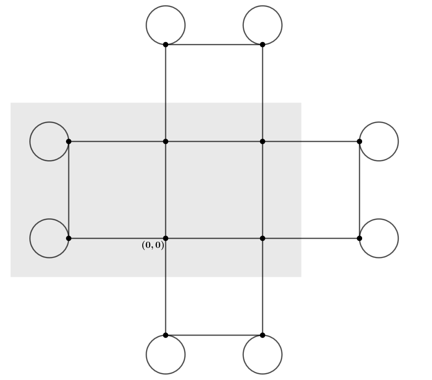 Figure 1
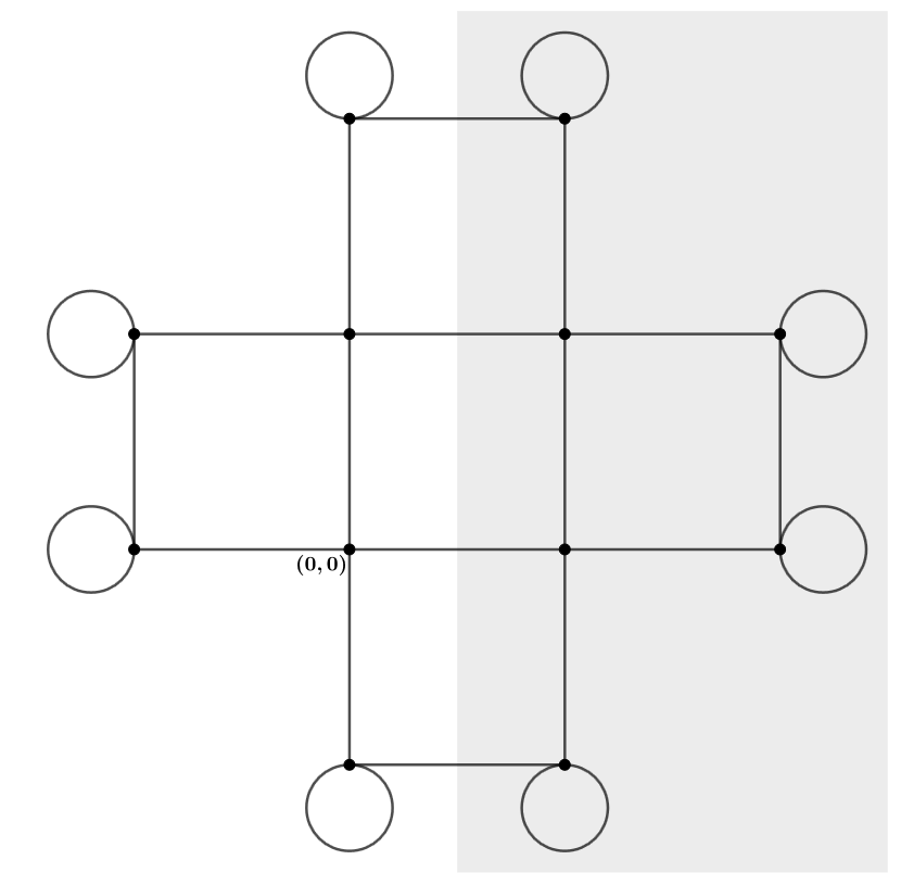 Figure 2
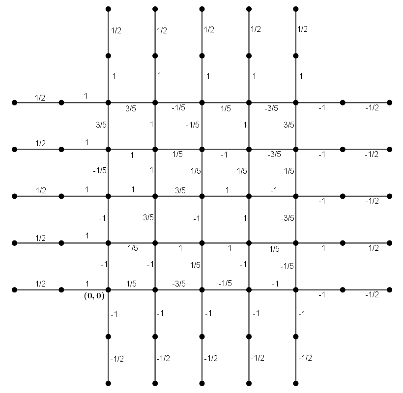 Figure 3
Peer Reviews
No public reviews on file for this paper yet. If you reviewed it on a platform where reviews are public (OpenReview, ICLR, NeurIPS, ICML), you can paste yours below so the community can read it here.
Videos
No videos yet. Explain this paper in a talk, walkthrough, or lecture? Add one.
The Total Variation Flow in Metric Random Walk Spaces
José M. Mazón, Marcos Solera and Julián Toledo
J. M. Mazón: Departament d’Anàlisi Matemàtica, Universitat de València, Dr. Moliner 50, 46100 Burjassot, Spain. [email protected]
M. Solera: Departament d’Anàlisi Matemàtica, Universitat de València, Dr. Moliner 50, 46100 Burjassot, Spain. [email protected]
J. Toledo: Departament d’Anàlisi Matemàtica, Universitat de València, Dr. Moliner 50, 46100 Burjassot, Spain. [email protected]
Abstract.
In this paper we study the Total Variation Flow (TVF) in metric random walk spaces, which unifies into a broad framework the TVF on locally finite weighted connected graphs, the TVF determined by finite Markov chains and some nonlocal evolution problems. Once the existence and uniqueness of solutions of the TVF has been proved, we study the asymptotic behaviour of those solutions and, with that aim in view, we establish some inequalities of Poincaré type. In particular, for finite weighted connected graphs, we show that the solutions reach the average of the initial data in finite time. Furthermore, we introduce the concepts of perimeter and mean curvature for subsets of a metric random walk space and we study the relation between isoperimetric inequalities and Sobolev inequalities. Moreover, we introduce the concepts of Cheeger and calibrable sets in metric random walk spaces and characterize calibrability by using the -Laplacian operator. Finally, we study the eigenvalue problem whereby we give a method to solve the optimal Cheeger cut problem.
Key words and phrases:
Random walk, Total variation flow, Sets of finite perimeter, Nonlocal operators, Cheeger sets, Calibrable sets, Functions of bounded variation.
2010 Mathematics Subject Classification: 05C80, 35R02, 05C21, 45C99, 26A45.
Contents
-
2 Perimeter, Curvature and Total Variation in Metric Random Walk Spaces
-
3 The -Laplacian and the Total Variation Flow in Metric Random Walk Spaces
-
4 Asymptotic Behaviour of the TVF and Poincaré type Inequalities
-
6 The Eigenvalue Problem for the -Laplacian in Metric Random Walk Spaces
-
6.1 The -Cheeger Constant of a Metric Random Walk Space with Finite Measure
1. Introduction and Preliminaries
A metric random walk space is a metric space together with a family of probability measures that encode the jumps of a Markov chain. Important examples of metric random walk spaces are: locally finite weighted connected graphs, finite Markov chains and with the Euclidean distance and
[TABLE]
where is a measurable, nonnegative and radially symmetric function with . Furthermore, given a metric measure space satisfying certain properties we can obtain a metric random walk space , called the -step random walk associated to , where
[TABLE]
Since its introduction as a means of solving the denoising problem in the seminal work by Rudin, Osher and Fatemi ([49]), the total variation flow has remained one of the most popular tools in Image Processing. Recall that, from the mathematical point of view, the study of the total variation flow in was established in [5]. On the other hand, the use of neighbourhood filters by Buades, Coll and Morel in [12], that was originally proposed by P. Yaroslavsky ([52]), has led to an extensive literature in nonlocal models in image processing (see for instance [8], [29], [32], [33] and the references therein). Consequently, there is great interest in studying the total variation flow in the nonlocal context. As further motivation, note that an image can be considered as a weighted graph, where the pixels are taken as the vertices and the “similarity” between pixels as the weights. The way in which these weights are defined depends on the problem at hand, see for instance [24] and [33].
The aim of this paper is to study the total variation flow in metric random walk spaces, obtaining general results that can be applied, for example, to the different points of view in Image Processing. In this regard, we introduce the -Laplacian operator associated with a metric random walk space, as well as the notions of perimeter and mean curvature for subsets of a metric random walk space. In doing so, we generalize results obtained in [36] and [37] for the particular case of , and, moreover, generalize results in graph theory. We then proceed to prove existence and uniqueness of solutions of the total variation flow in metric random walk spaces and to study its asymptotic behaviour with the help of some Poincaré type inequalities. Furthermore, we introduce the concepts of Cheeger and calibrable sets in metric random walk spaces and characterize calibrability by using the -Laplacian operator. Let us point out that, to our knowledge, some of these results were not yet known for graphs, nonetheless, we have specified in the main text which important results were already known for graphs. Moreover, in the forthcoming paper [39], we apply the theory developed here to obtain the -decomposition, , of functions in metric random walk spaces. This decomposition can be applied to Image Processing if, for example, images are regarded as graphs and, moreover, to other nonlocal models.
Partitioning data into sensible groups is a fundamental problem in machine learning, computer science, statistics and science in general. In these fields, it is usual to face large amounts of empirical data, and getting a first impression of the data by identifying groups with similar properties can prove to be very useful. One of the most popular approaches to this problem is to find the best balanced cut of a graph representing the data, such as the Cheeger ratio cut ([17]). Consider a finite weighted connected graph , where is the set of vertices (or nodes) and the set of edges, which are weighted by a function , . The degree of the vertex is denoted by , . In this context, the Cheeger cut value of a partition () of is defined as
[TABLE]
where
[TABLE]
and is the volume of , defined as . Furthermore,
[TABLE]
is called the Cheeger constant, and a partition of is called a Cheeger cut of if . Unfortunately, the Cheeger minimization problem of computing is NP-hard ([30], [48]). However, it turns out that can be approximated by the second eigenvalue of the graph Laplacian thanks to the following Cheeger inequality ([18]):
[TABLE]
This motivates the spectral clustering method ([34]), which, in its simplest form, thresholds the second eigenvalue of the graph Laplacian to get an approximation to the Cheeger constant and, moreover, to a Cheeger cut. In order to achieve a better approximation than the one provided by the classical spectral clustering method, a spectral clustering based on the graph -Laplacian was developed in [13], where it is showed that the second eigenvalue of the graph -Laplacian tends to the Cheeger constant as . In [48] the idea was taken up by directly considering the variational characterization of the Cheeger constant
[TABLE]
where
[TABLE]
The subdifferential of the energy functional is the -Laplacian in graphs . Using the nonlinear eigenvalue problem , the theory of -Spectral Clustering is developed in [14], [15], [16] and [30], and good results on the Cheeger minimization problem have been obtained.
In [38], we obtained a generalization, in the framework of metric random walk spaces, of the Cheeger inequality (1.1) and of the variational characterization of the Cheeger constant (1.2). In this paper, in connection with the -Spectral Clustering, also in metric random walk spaces, we study the eigenvalue problem of the -Laplacian and then relate it to the optimal Cheeger cut problem. Then again, these results apply, in particular, to locally finite weighted connected graphs, complementing the results given in [14], [15], [16] and [30].
Additionally, regarding the notion of a function of bounded variation in a metric measure space introduced by Miranda in [43], we provide, via the -step random walk associated to , a characterization of these functions.
1.1. Metric Random Walk Spaces
Let be a Polish metric space equipped with its Borel -algebra. A random walk on is a family of probability measures on , , satisfying the two technical conditions: (i) the measures depend measurably on the point , i.e., for any Borel set of and any Borel set of , the set is Borel; (ii) each measure has finite first moment, i.e. for some (hence any, by the triangle inequality) , and for any one has (see [46]).
A metric random walk space is a Polish metric space together with a random walk on .
Let be a metric random walk space. A Radon measure on is invariant for the random walk if
[TABLE]
that is, for any -measurable set , it holds that is -measurable for -almost all , is -measurable, and
[TABLE]
Consequently, if is an invariant measure with respect to and , it holds that for -a.e. , is -measurable, and
[TABLE]
The measure is said to be reversible for if, moreover, the following detailed balance condition holds:
[TABLE]
that is, for any Borel set ,
[TABLE]
where \raisebox{2.0pt}{\rm{\chi}}_{C} is the characteristic function of the set defined as
[TABLE]
Note that the reversibility condition implies the invariance condition. However, we will sometimes write that is invariant and reversible so as to emphasize both conditions.
We now give some examples of metric random walk spaces that illustrate the general abstract setting. In particular, Markov chains serve as paradigmatic examples that capture many of the properties of this general setting that we will encounter during our study.
Example 1.1**.**
(1) Consider , with the Euclidean distance and the Lebesgue measure. For simplicity we will write instead of . Let be a measurable, nonnegative and radially symmetric function verifying . In we have the following random walk, starting at ,
[TABLE]
Applying Fubini’s Theorem it is easy to see that the Lebesgue measure is an invariant and reversible measure for this random walk.
Observe that, if we assume that in we have an homogeneous population and is thought of as the probability distribution of jumping from location to location , then, for a Borel set in , is measuring how many individuals are going to from following the law given by . See also the interpretation of the -interaction between sets given in Section 2.1. Finally, note that the same ideas are applicable to the countable spaces given in the following two examples.
(2) Let be a Markov kernel on a countable space , i.e.,
[TABLE]
Then, for
[TABLE]
* is a metric random walk space for any metric on .*
Moreover, in Markov chain theory terminology, a measure on satisfying
[TABLE]
is called a stationary probability measure (or steady state) on . This is equivalent to the definition of invariant probability measure for the metric random walk space . In general, the existence of such a stationary probability measure on is not guaranteed. However, for irreducible and positive recurrent Markov chains (see, for example, [31] or [45]) there exists a unique stationary probability measure.
Furthermore, a stationary probability measure is said to be reversible for if the following detailed balance equation holds:
[TABLE]
By Tonelli’s Theorem for series, this balance condition is equivalent to the one given in (1.3) for :
[TABLE]
(3) Consider a locally finite weighted discrete graph , where each edge (we will write if ) has a positive weight assigned. Suppose further that if .
A finite sequence of vertices on the graph is called a path if for all . The length of a path is defined as the number of edges in the path. Then, is said to be connected if, for any two vertices , there is a path connecting and , that is, a path such that and . Finally, if is connected, define the graph distance between any two distinct vertices as the minimum of the lengths of the paths connecting and . Note that this metric is independent of the weights. We will always assume that the graphs we work with are connected.
For we define the weight at the vertex as
[TABLE]
and the neighbourhood of as . Note that, by definition of locally finite graph, the sets are finite. When for every , coincides with the degree of the vertex in a graph, that is, the number of edges containing vertex .
For each we define the following probability measure
[TABLE]
We have that is a metric random walk space and it is not difficult to see that the measure defined as
[TABLE]
is an invariant and reversible measure for this random walk.
Given a locally finite weighted discrete graph , there is a natural definition of a Markov chain on the vertices. We define the Markov kernel as
[TABLE]
We have that and define the same random walk. If is finite, the unique stationary and reversible probability measure is given by
[TABLE]
(4) From a metric measure space we can obtain a metric random walk space, the so called -step random walk associated to , as follows. Assume that balls in have finite measure and that . Given , the -step random walk on starting at , consists in randomly jumping in the ball of radius centered at with probability proportional to ; namely
[TABLE]
Note that is an invariant and reversible measure for the metric random walk space .
(5) Given a metric random walk space with invariant and reversible measure , and given a -measurable set with , if we define, for ,
[TABLE]
we have that is a metric random walk space and it easy to see that is reversible for .
In particular, if is a closed and bounded subset of , we obtain the metric random walk space , where , that is
[TABLE]
From this point onwards, when dealing with a metric random walk space, we will assume that there exists an invariant and reversible measure for the random walk, which we will always denote by . In this regard, when it is clear from the context, a measure denoted by will always be an invariant and reversible measure for the random walk under study. Furthermore, we assume that the metric measure space is -finite.
1.2. Completely Accretive Operators and Semigroup Theory
Since Semigroup Theory will be used along the paper, we would like to conclude this introduction with some notations and results from this theory along with results from the theory of completely accretive operators (see [9], [10] and [22], or the Appendix in [6], for more details). We denote by and the following sets of functions:
[TABLE]
[TABLE]
Let . The following relation between and is defined in [9]:
[TABLE]
An operator is called completely accretive if
[TABLE]
and every , . Moreover, an operator in is m-completely accretive in if is completely accretive and for all (or, equivalently, for some ).
Theorem 1.2** ([9], [10]).**
If is an m-completely accretive operator in , then, for every (the closure of the domain of ), there exists a unique mild solution (see [22]) of the problem
[TABLE]
Moreover, if is the subdifferential of a proper convex and lower semicontinuous function in then the mild solution of the above problem is a strong solution.
Furthermore we have the following contraction and maximum principle in any space, : for and denoting by the unique mild solution of the problem
[TABLE]
* we have*
[TABLE]
where for .
2. Perimeter, Curvature and Total Variation in Metric Random Walk Spaces
2.1. -Perimeter
Let be a metric random walk space with invariant and reversible measure . We define the -interaction between two -measurable subsets and of as
[TABLE]
Whenever , by the reversibility assumption on with respect to , we have
[TABLE]
Following the interpretation given after Example 1.1 (1), for a -homogeneous population which moves according to the law provided by the random walk , measures how many individuals are moving from to , and, thanks to the reversibility, this is equal to the amount of individuals moving from to . In this regard, the following concept measures the total flux of individuals that cross the “boundary” (in a very weak sense) of a set.
We define the concept of -perimeter of a -measurable subset as
[TABLE]
It is easy to see that
[TABLE]
Moreover, if is -integrable, we have
[TABLE]
The notion of -perimeter can be localized to a bounded open set by defining
[TABLE]
Observe that
[TABLE]
and, consequently, we have
[TABLE]
when both integrals are finite.
Example 2.1**.**
(1) Let be the metric random walk space given in Example 1.1 (1) with invariant measure . Then,
[TABLE]
which coincides with the concept of -perimeter introduced in [36]. On the other hand,
[TABLE]
Note that, in general,
Moreover,
[TABLE]
and, therefore,
[TABLE]
(2) In the case of the metric random walk space associated to a finite weighted discrete graph , given , is defined as
[TABLE]
and the perimeter of a set is given by
[TABLE]
Consequently, we have that
[TABLE]
Let us now give some properties of the -perimeter.
Proposition 2.2**.**
Let be -measurable sets with finite -perimeter such that . Then,
[TABLE]
Proof.
We have
[TABLE]
and then, by the reversibility assumption on with respect to ,
[TABLE]
Corollary 2.3**.**
Let be -measurable sets in with pairwise -null intersections. Then
[TABLE]
2.2. -Mean Curvature
Let be -measurable. For a point we define the -mean curvature of at as
[TABLE]
Observe that
[TABLE]
Note that can be computed for every , not only for points in . This fact will be used later in the paper. Having in mind (2.3), we have that, for a –integrable set ,
[TABLE]
[TABLE]
Consequently,
[TABLE]
2.3. -Total Variation
Associated to the random walk and the invariant measure , we define the space
[TABLE]
We have that . The -total variation of a function is defined by
[TABLE]
Note that
[TABLE]
Observe that the space is the nonlocal counterpart of classical local bounded variation spaces. Note further that, in the local context, given a Lebesgue measurable set , its perimeter is equal to the total variation of its characteristic function (see (2.35)) and the above equation (2.12) provides the nonlocal counterpart. In (2.40) and Theorem 2.22 we illustrate further relations between these spaces.
However, although they represent analogous concepts in different settings, the classical local BV-spaces and the nonlocal BV-spaces are of a different nature. For example, in our nonlocal framework in contrast with classical local bounded variation spaces that are, by definition, contained in . Indeed, since each is a probability measure, , and is invariant with respect to , we have that
[TABLE]
Recall the definition of the generalized product measure (see, for instance, [3]), which is defined as the measure on given by
[TABLE]
where it is required that the map is -measurable for any Borel set . Moreover, it holds that
[TABLE]
for every . Therefore, we can write
[TABLE]
Example 2.4**.**
Let be the metric random walk space given in Example 1.1 (3) with invariant and reversible measure . Then,
[TABLE]
[TABLE]
which coincides with the anisotropic total variation defined in [28].
In the following results we give some properties of the total variation.
Proposition 2.5**.**
If is Lipschitz continuous then, for every , and
[TABLE]
Proof.
[TABLE]
[TABLE]
Proposition 2.6**.**
* is convex and continuous in .*
Proof.
Convexity follows easily. Let us see that it is continuous. Let in . Since is invariant and reversible with respect to , we have
[TABLE]
[TABLE]
[TABLE]
As in the local case, we have the following coarea formula relating the total variation of a function with the perimeter of its superlevel sets.
Theorem 2.7** **(Coarea formula).
For any , let . Then,
[TABLE]
Proof.
Since
[TABLE]
we have
[TABLE]
Moreover, since implies \raisebox{2.0pt}{\rm{\chi}}_{E_{t}(u)}(y)\geq\raisebox{2.0pt}{\rm{\chi}}_{E_{t}(u)}(x), we obtain that
[TABLE]
Therefore, we get
[TABLE]
where Tonelli-Hobson’s Theorem is used in the third equality.
Let us recall the following concept of -connectedness introduced in [36]: A metric random walk space with invariant and reversible measure is -connected if, for any pair of -non-null measurable sets such that , we have . Moreover, in [38, Theorem 2.19], we see that this concept is equivalent to the following concept of ergodicity (see [31]) when is a probability measure.
Definition 2.8**.**
Let be a metric random walk space with invariant and reversible probability measure . A Borel set is said to be invariant with respect to the random walk if whenever is in . The invariant probability measure is said to be ergodic if or for every invariant set with respect to the random walk .
Furthermore, by [38, Theorem 2.21], we have that is ergodic if, and only if, for , implies that is -a.e. equal to a constant, where
[TABLE]
As an example, note that the metric random walk space associated to an irreducible and positive recurrent Markov chain on a countable space together with its steady state is -connected (see [31]). Moreover, the metric random walk space associated to a locally finite weighted connected discrete graph is -connected. In [38] we give further examples involving the metric random walk space given in Example 1.1 (1).
Observe that, for a metric random walk space with invariant and reversible measure , if the space is -connected, then the -perimeter of any -measurable set with is positive.
Lemma 2.9**.**
Assume that is ergodic and let . Then,
[TABLE]
Proof.
() Suppose that is -a.e. equal to a constant , then, since is invariant with respect to , we have
[TABLE]
() Suppose that
[TABLE]
Then, for -a.e. , thus
[TABLE]
and we are done by the comments preceding the lemma.
From now on we will assume that the metric random walk spaces that we work with are -connected (this assumption is only dropped in subsection 2.5). However, we would like to point out that if a metric random walk space is not -connected then it may be broken down as where , have -positive measure and , allowing us to work with and independently. Then, for example, if is a -measurable set we get
[TABLE]
and, if ,
[TABLE]
2.4. Isoperimetric and Sobolev inequalities
The -dimensional isoperimetric inequality states that
[TABLE]
for every domain with smooth boundary and compact closure, where , and is the volume of the unit ball. It is well known (see for instance [41]) that (2.16) is equivalent to the *Sobolev inequality *
[TABLE]
If we replace the Euclidean space by a Riemannian manifold with measure , then the isoperimetric inequality takes the following form:
[TABLE]
for all bounded sets with smooth boundary, being the surface measure. As in the Euclidean case (see [40] or [47]), (2.18) is equivalent to the Sobolev inequality
[TABLE]
Consequently, it is natural to say that a Riemannian manifold has isoperimetric dimension if (2.19) holds (see [21]). The equivalence between isoperimetric inequalities and Sobolev inequalities in the context of Markov chains was obtained by Varopoulos in [51]. Let us state these results under the context treated here.
Definition 2.10**.**
Let be a metric random walk space with invariant and reversible measure . We say that has isoperimetric dimension if there exists a constant such that
[TABLE]
We assume that, for , by convention.
We will denote by the set of functions satisfying that there exists , with , such that in .
Theorem 2.11**.**
* has isoperimetric dimension if, and only if,*
[TABLE]
The constant is the same as in (2.20).
Proof.
() Given with , applying (2.21) to \raisebox{2.0pt}{\rm{\chi}}_{A}, we get
[TABLE]
() Let us see that (2.20) implies (2.21). Since , we may assume that without loss of generality.
Suppose first that and let such that and is not -a.e. equal to [math] (otherwise, (2.21) is trivially satisfied). Note that, in this case, since is null outside of a -measurable set with , we have for and, moreover, by the definition of the -norm, for . Then, by the coarea formula and (2.20), we have
[TABLE]
Therefore, we may suppose that . Let . Again, by the coarea formula and (2.20), if , and not identically -null, we get
[TABLE]
where if . On the other hand, since the function is nonnegative and non-increasing, we have
[TABLE]
Integrating over and letting , we obtain
[TABLE]
that is,
[TABLE]
Now,
[TABLE]
[TABLE]
Thus, by (2.23), we get
[TABLE]
Finally, from (2.22) and (2.24), we obtain (2.21).
Note that, if we take , we can rewrite (2.20) as
[TABLE]
The next definition was given in [21] for Riemannian manifolds.
Definition 2.12**.**
Given a non-increasing function , we say that satisfies a -isoperimetric inequality if
[TABLE]
Example 2.13**.**
(1) In [50] (see also the references therein) it is shown that the lattice has isoperimetric dimension with constant , and that the complete graph satisfies a -isoperimetric inequality with . In addition, it is also proved that the -cube satisfies a -isoperimetric inequality with .
(2) In **[37]**, for , it is proved that
[TABLE]
being
[TABLE]
where is the ball of radius centered at [math] and is the -mean curvature of (see Subsection 2.2). Therefore, satisfies a -isoperimetric inequality, where is a decreasing function.
The next result was proved in [21] for Riemannian manifolds and in [20] for graphs (see also [50, Theorem 2]).
Proposition 2.14**.**
Given a non-increasing function , we have that satisfies a -isoperimetric inequality if, and only if, the following inequality holds:
[TABLE]
for all -measurable sets with and all with
Proof.
Taking u=\raisebox{2.0pt}{\rm{\chi}}_{A} in (2.29), we obtain that satisfies a -isoperimetric inequality. Conversely, since , it is enough to prove (2.29) for . If in the result is trivial. Therefore, let be a -measurable set with and a non--null function with . For we have that and, therefore, , thus, since is non-increasing, we have that . Therefore, by the coarea formula, we have
[TABLE]
As a consequence of Theorem 2.11 and Proposition 2.14, we obtain the following result.
Corollary 2.15**.**
The following assertions are equivalent:
*(i)
(ii) for all with and all with in
Consider the Dirichlet energy functional defined as
[TABLE]
The next result, in the context of Markov chains, was obtained by Varopoulos in [51].
Theorem 2.16**.**
Let . If the Sobolev inequality
[TABLE]
holds, then there exists such that
[TABLE]
Proof.
We can assume that . Let . By (2.30), we have
[TABLE]
On the other hand, since, for ,
[TABLE]
by the convexity of , and having in mind the reversibility of , we have
[TABLE]
[TABLE]
[TABLE]
[TABLE]
Then, by (2.32), we get
[TABLE]
Now,
[TABLE]
thus, from (2.33),
[TABLE]
and, therefore,
[TABLE]
where
Following Theorem 2.11 and Theorem 2.16 we can also obtain a Sobolev inequality as a consequence of the isoperimetric dimensional inequality.
Corollary 2.17**.**
Assume that . Let . If has isoperimetric dimension then there exists such that
[TABLE]
Let us point out that an important consequence of this result is Theorem 5 in [19], which corresponds to Corollary 2.17 for the particular case of finite weighted graphs.
2.5. - versus in Metric Measure Spaces
Let be a metric measure space and recall that, for functions in , Miranda introduced a local notion of total variation in [43] (see also [2]). To define this notion, first note that for a function , its slope (or local Lipschitz constant) is defined as
[TABLE]
with the convention that if is an isolated point.
A function is said to be a BV-function if there exists a sequence of locally Lipschitz functions converging to in and such that
[TABLE]
We shall denote the space of all BV-functions by . Let , the total variation of on an open set is defined as:
[TABLE]
A set is said to be of finite perimeter if \raisebox{2.0pt}{\rm{\chi}}_{E}\in BV(X,d,\nu) and its perimeter is defined as
[TABLE]
We want to point out that in [2] the BV-functions are characterized using different notions of total variation.
As aforementioned, the local classical BV-spaces and the nonlocal BV-spaces are of different nature although they represent analogous concepts in different settings. In this section we compare these spaces, showing that it is possible to relate the nonlocal concept to the local one after rescaling and taking limits.
Remark 2.18**.**
Obviously,
[TABLE]
Furthermore, there exist metric measures spaces in which the equality in this expression does not hold (see [4, Remark 4.4]).
Proposition 2.19**.**
Let be a metric random walk space with invariant and reversible measure . Let . Then for -a.e. and
[TABLE]
Proof.
Since , there exists a sequence such that
[TABLE]
Now, using the invariance of ,
[TABLE]
Therefore, we may take a subsequence, which we still denote by , such that for -a.e. .
Moreover, by Fatou’s lemma and the invariance of ,
[TABLE]
Consequently, and in for -a.e. , thus for -a.e. , and
[TABLE]
It is shown in [37] that, in the context of Example 1.1 (1), and assuming that satisfies
[TABLE]
we have that
[TABLE]
for every .
In the next example we see that there exist metric random walk spaces in which it is not possible to obtain an inequality like (2.39).
Example 2.20**.**
Let be a locally finite weighted discrete graph with weights . For a fixed the function u=\raisebox{2.0pt}{\rm{\chi}}_{\{x_{0}\}} is a Lipschitz function and, since every vertex is isolated for the graph distance, , thus
[TABLE]
However, by Example 2.4, we have
[TABLE]
Let be the metric random walk space of Example 1.1 (1). Then, if is compactly supported and has compact support we have that (see [23] and [36])
[TABLE]
where
[TABLE]
In particular, if we take
[TABLE]
then
[TABLE]
Hence,
[TABLE]
and, consequently, by (2.40), we have
[TABLE]
Therefore, it is natural to pose the following problem: Let be a metric measure space and let be the -step random walk associated to , that is,
[TABLE]
Are there metric measure spaces for which
[TABLE]
To give a positive answer to the previous question we recall the following concepts on a metric measure space : The measure is said to be doubling if there exists a constant such that
[TABLE]
A doubling measure has the following property. For every and if then
[TABLE]
where is a positive constant depending only on and .
On the other hand, the metric measure space is said to support a -Poincaré inequality if there exist constants and such that, for any , the inequality
[TABLE]
holds, where
[TABLE]
The following result is proved in [35, Theorem 3.1].
Theorem 2.21** ([35]).**
Let be a metric measure space with doubling and supporting a -Poincaré inequality. Given , we have that if, and only if,
[TABLE]
where . Moreover, there is a constant , that depends only on , such that
[TABLE]
Now, by Fubini’s Theorem, we have
[TABLE]
On the other hand, by (2.43), there exists a constant , depending only on , such that
[TABLE]
By (2.46), we have
[TABLE]
Hence, from (2.45) and (2.47), we get
[TABLE]
Therefore, we can rewrite Theorem 2.21 as follows.
Theorem 2.22**.**
Let be a metric measure space with doubling measure and supporting a -Poincaré inequality. Given , we have that if, and only if,
[TABLE]
Moreover, there is a constant , that depends only on , such that
[TABLE]
Remark 2.23**.**
Monti, in [44], defines
[TABLE]
and uses this to prove rearrangement theorems in the setting of metric measure spaces. Moreover, he proposes as a possible definition of the -length of the gradient of functions in metric measure spaces.
3. The -Laplacian and the Total Variation Flow in Metric Random Walk Spaces
Let be a metric random walk space with invariant and reversible measure . Assume, as aforementioned, that is -connected.
Given a function we define its nonlocal gradient as
[TABLE]
which should not be confused with the slope , , introduced in Section 2.5.
For a function , its -divergence is defined as
[TABLE]
and, for , we define the space
[TABLE]
Let and , , having in mind that is reversible, we have the following Green’s formula:
[TABLE]
In the next result we characterize and the -perimeter using the -divergence operator. Let us denote by the usual sign function and by the multivalued sign function:
[TABLE]
Proposition 3.1**.**
Let . For , we have
[TABLE]
In particular, for any -measurable set , we have
[TABLE]
Proof.
Let . Given with , applying Green’s formula (3.1), we have
[TABLE]
[TABLE]
Therefore,
[TABLE]
On the other hand, since is -finite, there exists a sequence of sets of -finite measure, such that . Then, if we define {\bf z}_{n}(x,y):={\rm sign}_{0}(u(y)-u(x))\raisebox{2.0pt}{\rm{\chi}}_{K_{n}\times K_{n}}(x,y), we have that with and
[TABLE]
Corollary 3.2**.**
* is lower semi-continuous with respect to the weak convergence in .*
Proof.
If weakly in then, given with , we have that
[TABLE]
by Proposition 3.3. Now, taking the supremum over in this inequality, we get
[TABLE]
Consider the formal nonlocal evolution equation
[TABLE]
In order to study the Cauchy problem associated to the previous equation, we will see in Theorem 3.8 that we can rewrite it as the gradient flow in of the functional defined by
[TABLE]
which is convex and lower semi-continuous. Following the method used in [5] we will characterize the subdifferential of the functional .
Given a functional , we define as
[TABLE]
with the convention that . Obviously, if , then .
Theorem 3.3**.**
Let and . The following assertions are equivalent:
(i) ;
(ii) there exists , such that
[TABLE]
and
[TABLE]
(iii) there exists , such that (3.6) holds and
[TABLE]
(iv) there exists antisymmetric with such that
[TABLE]
and
[TABLE]
(v) there exists antisymmetric with verifying (3.9) and
[TABLE]
Proof.
Since is convex, lower semi-continuous and positive homogeneous of degree , by [5, Theorem 1.8], we have
[TABLE]
We define, for ,
[TABLE]
Observe that is convex, lower semi-continuous and positive homogeneous of degree . Moreover, it is easy to see that, if , the infimum in (3.13) is attained i.e., there exists some such that and
Let us see that
[TABLE]
We begin by proving that . If then this assertion is trivial. Therefore, suppose that . Let such that . Then, for , we have
[TABLE]
Taking the supremum over we obtain that . Now, taking the infimum over , we get .
To prove the opposite inequality let us denote
[TABLE]
Then, by (3.2), we have that, for ,
[TABLE]
Thus, , which implies, by [5, Proposition 1.6], that . Therefore, , and, consequently, from (3.12), we get
[TABLE]
from where the equivalence between (i) and (ii) follows .
To prove the equivalence between (ii) and (iii) we only need to apply Green’s formula (3.1).
On the other hand, to see that (iii) implies (iv), it is enough to take . Moreover, to see that (iv) implies (ii), take (observe that, from (3.9), , so ). Finally, to see that (iv) and (v) are equivalent, we need to show that (3.10) and (3.11) are equivalent. Now, since g is antisymmetric with and is reversible, we have
[TABLE]
from where the equivalence between (3.10) and (3.11) follows.
By Theorem 3.3 and following [6, Theorem 7.5], the next result is easy to prove.
Proposition 3.4**.**
* is an m-completely accretive operator in .*
Definition 3.5**.**
We define in the multivalued operator by
* if, and only if, .*
As usual, we will write for .
Chang in [14] and Hein and Bühler in [30] define a similar operator in the particular case of finite graphs:
Example 3.6**.**
Let be the metric random walk given in Example 1.1 (3) with invariant measure . By Theorem 3.3, we have
[TABLE]
and
[TABLE]
The next example shows that the operator is indeed multivalued. Let and , , with . Then,
[TABLE]
and
[TABLE]
Now, since g is antisymmetric, we get
[TABLE]
Proposition 3.7**.**
[Integration by parts] For any it holds that
[TABLE]
and
[TABLE]
Proof.
Since , given , we have that
[TABLE]
so we get (3.14). On the other hand, (3.15) is given in Theorem 3.3.
As a consequence of Theorem 3.3, Proposition 3.4 and on account of Theorem 1.2, we can give the following existence and uniqueness result for the Cauchy problem
[TABLE]
which is a rewrite of the formal expression (3.4).
Theorem 3.8**.**
For every and any , there exists a unique solution of the Cauchy problem (3.16) in in the following sense: , in , and, for almost all ,
[TABLE]
Moreover, we have the following contraction and maximum principle in any –space, :
[TABLE]
for any pair of solutions, , of problem (3.16) with initial data respectively.
Definition 3.9**.**
Given , we denote by the unique solution of problem (3.16). We call the semigroup in the Total Variational Flow in the metric random walk space with invariant and reversible measure .
In the next result we give an important property of the total variational flow in metric random walk spaces.
Proposition 3.10**.**
The TVF satisfies the mass conservation property: for ,
[TABLE]
Proof.
By Proposition 3.7, we have
[TABLE]
and
[TABLE]
Hence,
[TABLE]
and, consequently,
[TABLE]
4. Asymptotic Behaviour of the TVF and Poincaré type Inequalities
Let be a metric random walk space with invariant and reversible measure . Assume as always that is -connected.
Proposition 4.1**.**
For every initial data ,
[TABLE]
with
[TABLE]
Moreover, if then
[TABLE]
Proof.
Since is a proper and lower semicontinuous function in attaining a minimum at the constant zero function and, moreover, is even, by [11, Theorem 5], we have
[TABLE]
with
[TABLE]
Now, since , we have that thus, by Lemma 2.9, if (then is ergodic) we get that is constant. Therefore, by Proposition 3.10,
[TABLE]
Let us see that we can get a rate of convergence of the total variational flow when a Poincaré type inequality holds.
From now on in this section we will assume that
[TABLE]
Hence, for all .
Definition 4.2**.**
We say that satisfies a -Poincaré inequality () if there exists a constant such that, for any ,
[TABLE]
or, equivalently (by the triangle inequality for one direction and taking for the other), there exists a such that
[TABLE]
where .
When satisfies a -Poincaré inequality, we will denote
[TABLE]
When satisfies a -Poincaré inequality, we will say that satisfies a -Poincaré inequality and write
[TABLE]
The following result was proved in [6, Theorem 7.11] for the particular case of the metric random walk space .
Theorem 4.3**.**
If satisfies a -Poincaré inequality, then, for any ,
[TABLE]
Proof.
Since the semigroup preserves the mass (Proposition 3.10), we have
[TABLE]
Furthermore, the complete accretivity of the operator (see Section 1.2) implies that
[TABLE]
is a Liapunov functional for the semigroup , which implies that
[TABLE]
Now, by the Poincaré inequality we get
[TABLE]
and, by (4.2) and (4.3), we obtain that
[TABLE]
On the other hand, by integration by parts (Proposition 3.7),
[TABLE]
and then
[TABLE]
which implies
[TABLE]
Hence, by (4.4)
[TABLE]
which concludes the proof.
To obtain a family of metric random walk spaces for which a -Poincaré inequality holds, we need the following result.
Lemma 4.4**.**
Suppose that is a probability measure (thus ergodic) and
[TABLE]
Let . Let be a bounded sequence in satisfying
[TABLE]
Then, there exists such that
[TABLE]
[TABLE]
Proof.
Let
[TABLE]
and
[TABLE]
From (4.6), it follows that
[TABLE]
Passing to a subsequence if necessary, we can assume that
[TABLE]
On the other hand, by (4.6), we also have that
[TABLE]
Therefore, we can suppose that, up to a subsequence,
[TABLE]
Let be a -null set satisfying that,
[TABLE]
Finally, set
Fix . Up to a subsequence we have that for some , but then, by (4.10), for every we also have that . However, since and , we have that ; thus, if then .
Let us see that
[TABLE]
Indeed, let . Then, for , , thus ; that is, , and, consequently, . Now, since , we have
[TABLE]
Therefore, since is ergodic, (4.13) implies that .
Consequently, we have obtained that converges -a.e. in to :
[TABLE]
Since is bounded, by Fatou’s Lemma, we must have that . On the other hand, by (4.9),
[TABLE]
for every . In other words, . Thus
[TABLE]
Theorem 4.5**.**
Suppose that is a probability measure and
[TABLE]
Let (H1) and (H2) denote the following hypothesis.
(H1) Given a -null set , there exist , -measurable sets and , such that and on , .
(H2) Let . Given a -null set , there exist and -measurable sets , such that and, for on , , .
Then, if (H1) holds, we have that satisfies a -Poincaré inequality for every , and, if (H2) holds, then satisfies a -Poincaré inequality.
Proof.
Let . We want to prove that there exists a constant such that
[TABLE]
for any when assuming and for the appearing in when this hypothesis is assumed. Suppose that this inequality is not satisfied. Then, there exists a sequence , with , satisfying
[TABLE]
and
[TABLE]
Therefore, by Lemma 4.4, there exist and a -null set such that
[TABLE]
We will now prove, distinguishing the cases in which we assume hypothesis or , that
[TABLE]
Suppose first that hypothesis is satisfied. Then, there exist , -measurable sets and , such that and on , . Note that, in this case, in the previous computations. Now,
[TABLE]
Consequently, since ,
[TABLE]
Therefore,
[TABLE]
Suppose now that hypothesis holds. Then, there exist , such that, given a -null set , there exist and -measurable sets , such that and, for on , , . Hence,
[TABLE]
Consequently, since ,
[TABLE]
Therefore,
[TABLE]
which concludes the proof of (4.19) in both cases.
Now, since , by (4.19) we get that , but this implies
[TABLE]
which is a contradiction with , , so we are done.
On account of Theorem 4.3, we obtain the following result on the asymptotic behaviour of the TVF.
Corollary 4.6**.**
Under the hypothesis of Theorem 4.5, for any ,
[TABLE]
Example 4.7**.**
We give two examples of metric random walk spaces in which a -Poincaré inequality does not hold.
(1) A locally finite weighted discrete graph with infinitely many vertices: Let be the metric random walk space associated to the locally finite weighted discrete graph with vertex set and weights:
[TABLE]
for , and otherwise (recall Example 1.1 (3)). Moreover, let
[TABLE]
Note that (we avoid its normalization for simplicity). Now,
[TABLE]
[TABLE]
[TABLE]
[TABLE]
However, we have
[TABLE]
thus
[TABLE]
where we use the notation
[TABLE]
Therefore,
[TABLE]
Finally,
[TABLE]
[TABLE]
Consequently,
[TABLE]
and a -Poincaré inequality does not hold for this space.
(2) The metric random walk space , where is the Euclidean distance and J(x)=\frac{1}{2}\raisebox{2.0pt}{\rm{\chi}}_{[-1,1]}: Define, for ,
[TABLE]
Then , and it is easy to see that, for large enough,
[TABLE]
Therefore, does not satisfy a -Poincaré inequality.
Let us see that, when satisfies a -Poincaré inequality, the solution of the Total Variational Flow reaches the steady state in finite time.
Theorem 4.8**.**
Let be a metric random walk space with invariant and reversible measure . If satisfies a -Poincaré inequality then, for any ,
[TABLE]
where is given in (4.1). Consequently,
[TABLE]
Proof.
Let , where . Since \Delta_{1}^{m}u(t)=\Delta_{1}^{m}\big{(}u(t)-\nu(u_{0})\big{)}, we have that
[TABLE]
Note that for every . Indeed, since is a maximal monotone operator in , by [10, Theorem 3.7] in the context of the Hilbert space , we have that for every .
Hence, for each , by Theorem 3.3, there exists antisymmetric with such that
[TABLE]
and
[TABLE]
Then, multiplying (4.27) by and integrating over with respect to , having in mind (4.28), we get
[TABLE]
Now, the semigroup preserves the mass (Proposition 3.10), so we have that for all , and, since satisfies a -Poincaré inequality, we have
[TABLE]
Therefore,
[TABLE]
Now, integrating this ordinary differential inequation we get
[TABLE]
that is,
[TABLE]
We define the extinction time as
[TABLE]
Under the conditions of Theorem 4.8, we have
[TABLE]
To obtain a lower bound on the extinction time, we introduce the following norm which, in the continuous setting, was introduced in [42]. Given a function , we define
[TABLE]
Theorem 4.9**.**
Let . If then
[TABLE]
Proof.
If , we have
[TABLE]
Then, by integration by parts (Proposition 3.7), we get
[TABLE]
[TABLE]
[TABLE]
[TABLE]
We will now see that we can get a -Poincaré inequality for finite graphs.
Theorem 4.10**.**
Let be a finite weighted connected discrete graph. Then, following the notation of Example 1.1 (3), satisfies a -Poincaré inequality, that is,
[TABLE]
Proof.
Let and suppose that (4.32) is false. Then, there exists a sequence with and , , such that
[TABLE]
Hence,
[TABLE]
Moreover, since , we have that, up to a subsequence,
[TABLE]
Now, since the graph is connected, we have that for , thus
[TABLE]
However, by the Dominated Convergence Theorem, we get that in and, therefore, since , we have , which is a contradiction with .
As a consequence of this last result and Theorem 4.8, we get:
Theorem 4.11**.**
Let be a finite weighted connected discrete graph. Then,
[TABLE]
where . Consequently,
[TABLE]
5. -Cheeger and -Calibrable Sets
Let be a metric random walk space with invariant and reversible measure . Assume, as before, that is -connected.
Given a set with , we define its -Cheeger constant by
[TABLE]
where the notation is chosen together with the one that we will use for the classical Cheeger constant (see (5.2)). In both of these, the subscript is there to further distinguish them from the upcoming notation for the -Cheeger constant of (see (6.11)). Note that, by (2.3), we have that .
A -measurable set achieving the infimum in (5.1) is said to be an -Cheeger set of . Furthermore, we say that is -calibrable if it is an -Cheeger set of itself, that is, if
[TABLE]
For ease of notation, we will denote
[TABLE]
for any -measurable set with .
Remark 5.1**.**
(1) Let be the metric random walk space given in Example 1.1 (1) with invariant and reversible measure . Then, the concepts of -Cheeger set and -calibrable set coincide with the concepts of -Cheeger set and -calibrable set introduced in [36] (see also [37]).
(2) If is a locally finite weighted discrete graph without loops (i.e., for all ) and more than two vertices, then any subset consisting of two vertices is -calibrable. Indeed, let , then, by (2.3), we have
[TABLE]
and, similarly,
[TABLE]
Therefore, is -calibrable.
In [36] it is proved that, for the metric random walk space , each ball is a -calibrable set. In the next example we will see that this result is not true in general.
Example 5.2**.**
Let be a finite weighted discrete graph with the following weights: and otherwise. Then, if , by (6.12) we have
[TABLE]
But, taking , we have
[TABLE]
Consequently, the ball is not -calibrable.
In the next Example we will see that there exist metric random walk spaces with sets that do not contain -Cheeger sets.
Example 5.3**.**
Consider the same graph of Example 6.21, that is, with the following weights:
[TABLE]
and otherwise. If , then for every with but, working as in Example 6.21, we get . Therefore, has no -cheeger set.
It is well known (see [25]) that the classical Cheeger constant
[TABLE]
for a bounded smooth domain , is an optimal Poincaré constant, namely, it coincides with the first eigenvalue of the -Laplacian:
[TABLE]
In order to get a nonlocal version of this result, we introduce the following constant. For with , we define
[TABLE]
Theorem 5.4**.**
Let with . Then,
[TABLE]
Proof.
Given a -measurable subset with , we have
[TABLE]
Therefore, . For the opposite inequality we will follow an idea used in [25]. Given , with in , and , we have
[TABLE]
[TABLE]
where the first equality follows by the coarea formula (2.14) and the last one by Cavalieri’s Principle. Taking the infimum over in the above expression we get .
Let us recall that, in the local case, a set is called calibrable if
[TABLE]
The following characterization of convex calibrable sets is proved in [1].
Theorem 5.5**.**
([1]) Given a bounded convex set of class , the following assertions are equivalent:
(a) is calibrable.
(b) \raisebox{2.0pt}{\rm{\chi}}_{\Omega} satisfies -\Delta_{1}\raisebox{2.0pt}{\rm{\chi}}_{\Omega}=\frac{\mbox{Per}(\Omega)}{|\Omega|}\raisebox{2.0pt}{\rm{\chi}}_{\Omega}, where .
(c)
Remark 5.6**.**
(1) Let be a -measurable set with and assume that there exists a constant and a measurable function such that for and
[TABLE]
Then, by Theorem 3.3, there exists antisymmetric with satisfying
[TABLE]
and
[TABLE]
Then,
[TABLE]
and, consequently,
[TABLE]
(2) Let be a -measurable set with , and a -measurable function with for . Then
[TABLE]
Indeed, the left to right implication follows from the fact that
[TABLE]
and for the converse implication, we have that there exists , for almost all , , satisfying
[TABLE]
Now, multiplying by \raisebox{2.0pt}{\rm{\chi}}_{\Omega}, integrating over and applying integrating by parts we get
[TABLE]
Then, since , the previous inequality is, in fact, an equality and, therefore, we get
[TABLE]
and, consequently,
[TABLE]
The next result is the nonlocal version of the fact that (a) is equivalent to (b) in Theorem 5.5.
Theorem 5.7**.**
Let be a -measurable set with . Then, the following assertions are equivalent:
(i) is -calibrable,
(ii) there exists a -measurable function equal to in such that
[TABLE]
(iii)
[TABLE]
for
[TABLE]
Proof.
Observe that, since we are assuming that the metric random walk space is -connected, we have and, therefore, .
is trivial.
: Suppose that there exists a -measurable function equal to in satisfying (5.6). Hence, there exists antisymmetric with satisfying
[TABLE]
and
[TABLE]
Then, for with , since antisymmetric, by using the reversibility of with respect to , we have
[TABLE]
Therefore, and, consequently, is -calibrable.
Suppose that is -calibrable. Let
[TABLE]
We claim that , that is,
[TABLE]
Take with . Since
[TABLE]
and
[TABLE]
we have
[TABLE]
Now, using that in and is -calibrable we have that
[TABLE]
By Proposition 2.2 and the coarea formula given in Theorem 2.7 we get
[TABLE]
Hence, if we prove that
[TABLE]
we get
[TABLE]
which proves (5.10). Now, since
[TABLE]
and for , we have
[TABLE]
Then, by (5.5), we have that
[TABLE]
and this concludes the proof.
Even though, in principle, the -calibrability of a set is a nonlocal concept, in the next result we will see that the -calibrability of a set depends only on the set itself.
Theorem 5.8**.**
Let be a -measurable set with . Then, is -calibrable if, and only if, there exists an antisymmetric function in such that
[TABLE]
and
[TABLE]
Observe that, on account of (2.3), (5.13) is equivalent to
[TABLE]
Proof.
By Theorem 5.7, we have that is -calibrable if, and only if, there exists antisymmetric, with g(x,y)\in{\rm sign}(\raisebox{2.0pt}{\rm{\chi}}_{\Omega}(y)-\raisebox{2.0pt}{\rm{\chi}}_{\Omega}(x)) for -a.e. , satisfying
[TABLE]
and
[TABLE]
Now, having in mind that if and , we have that, for ,
[TABLE]
[TABLE]
Bringing together (5.15) and these equalities we get (5.12) and (5.13).
Let us now suppose that we have an antisymmetric function in satisfying (5.12) and (5.13). To check that is -calibrable we need to find \tilde{\bf g}(x,y)\in\hbox{sign}\left(\raisebox{2.0pt}{\rm{\chi}}_{\Omega}(y)-\raisebox{2.0pt}{\rm{\chi}}_{\Omega}(x)\right) antisymmetric such that
[TABLE]
which is equivalent to
[TABLE]
since, necessarily, for and , and for and . Now, the second equality in this system is satisfied if we take for , and the first one is equivalent to (5.14) if we take for .
Set
[TABLE]
where
[TABLE]
Corollary 5.9**.**
A -measurable set is -calibrable if, and only if, it is -calibrable as a subset of with reversible measure (see Example 1.1 (5)).
Remark 5.10**.**
(1) Let be a -measurable set with . Observe that, as we have proved,
[TABLE]
(2) Let be a -measurable set. If
[TABLE]
*for some -measurable function , then there exists antisymmetric with
satisfying*
[TABLE]
and
[TABLE]
Hence, if
[TABLE]
we have that
[TABLE]
Indeed, from (5.19), for ,
[TABLE]
Hence, integrating over with respect to , we get
[TABLE]
Moreover, since is antisymmetric and -integrable, we have
[TABLE]
and, consequently, we get
[TABLE]
As a consequence of (5.20), if , since the metric random walk space is -connected, the relation
[TABLE]
does not hold true for any -measurable set with (recall that, for these , by [38, Theorem 2.21&2.24] thus is non–null by (5.20)). Now, if , then (5.21) may be satisfied, as shown in the next example.
Example 5.11**.**
Consider the metric random walk space with and J=\frac{1}{2}\raisebox{2.0pt}{\rm{\chi}}_{[-1,1]}. Let us see that
[TABLE]
where . Indeed, take to be antisymmetric and defined as follows for :
[TABLE]
Then, , ,
[TABLE]
and
[TABLE]
Note that is not integrable.
Remark 5.12**.**
As a consequence of Theorem 5.5, it holds that (see [1, Introduction] or [5, Section 4.4]) a bounded convex set is calibrable if, and only if, u(t,x)=\left(1-\frac{\mbox{Per}(\Omega)}{|\Omega|}t\right)^{+}\raisebox{2.0pt}{\rm{\chi}}_{\Omega}(x) is a solution of the Cauchy problem
[TABLE]
That is, a calibrable set is that for which the gradient descent flow associated to the total variation tends to decrease linearly the height of \raisebox{2.0pt}{\rm{\chi}}_{\Omega} without distortion of its boundary.
Now, as a consequence of (5.18), we can obtain a similar result in our context if we introduce an abortion term in the corresponding Cauchy problem. The appearance of this term is due to the nonlocality of the diffusion considered. Let be a -measurable set with , then is -calibrable if, and only if, u(t,x)=\left(1-\lambda^{m}_{\Omega}t\right)^{+}\raisebox{2.0pt}{\rm{\chi}}_{\Omega}(x) is a solution of
[TABLE]
Note that the only if direction follows by the uniqueness of the solution.
The following result relates the -calibrability with the -mean curvature, this is the nonlocal version of one of the implications in the equivalence between (a) and (c) in Theorem 5.5.
Proposition 5.13**.**
Let be a -measurable set with . Then,
[TABLE]
Equivalently,
[TABLE]
Proof.
By Theorem 5.8, there exists an antisymmetric function in such that
[TABLE]
and
[TABLE]
Hence,
[TABLE]
from where (5.24) follows.
The equivalent thesis (5.25) follows from (5.24) and the fact that
\hbox{\nu\underset{x\in\Omega}{\rm ess,sup}\ H^{m}{\partial\Omega}(x)}\leq\lambda^{m}_{\Omega} \displaystyle\frac{1}{\nu(\Omega)}\int_{\Omega}m_{x}(\Omega)d\nu(x)\leq 2\,\hbox{\nu\underset{x\in\Omega}{\rm ess\ inf}\ m{x}(\Omega)}.
For this last equivalence recall from (2.10) that
[TABLE]
and that
[TABLE]
The converse of Proposition 5.13 is not true in general, an example is given in [36] (see also [37]) for , with the Euclidean distance and J=\frac{1}{|B_{1}(0)|}\raisebox{2.0pt}{\rm{\chi}}_{B_{1}(0)}. Let us see an example, in the case of graphs, where the converse of Proposition 5.13 is not true
Example 5.14**.**
Let be a finite weighted discrete graph with the following weights: and otherwise. If , we have
[TABLE]
Therefore, (5.25) holds. However, is not -calibrable since, if , we have
[TABLE]
Proposition 5.15**.**
Let be a -measurable set with .
(1) If with , , , and (whenever this non-trivial decomposition is satisfied we will write ), then
[TABLE]
(2) If is -calibrable, then each is -calibrable, , and
[TABLE]
Proof.
(1) is a direct consequence of Proposition 2.2 and the fact that, for positive real numbers, (2) is a direct consequence of (1) together with the definition of -calibrability.
6. The Eigenvalue Problem for the -Laplacian in Metric Random Walk Spaces
Let be a metric random walk space with invariant and reversible measure and assume that is -connected.
In this section we introduce the eigenvalue problem associated with the -Laplacian and its relation with the Cheeger minimization problem. For the particular case of finite weighted discrete graphs where the weights are either [math] or , this problem was first studied by Hein and Bühler ([30]) and a more complete study was subsequently performed by Chang in [14].
Definition 6.1**.**
A pair is called an -eigenpair of the -Laplacian on if and there exists (i.e., for every ) such that
[TABLE]
The function is called an -eigenfunction and an -eigenvalue associated to .
Observe that, if is an -eigenpair of , then is also an -eigenpair of .
Remark 6.2**.**
By Theorem 3.3, the following statements are equivalent:
(1) is an -eigenpair of the -Laplacian .
(2) There exists antisymmetric with , such that
[TABLE]
(3) There exists antisymmetric with , such that
[TABLE]
(4) There exists antisymmetric with , such that
[TABLE]
Remark 6.3**.**
Note that, since for any -eigenpair of , then
[TABLE]
thus
[TABLE]
Example 6.4**.**
Let be the metric random walk space given in Example 1.1 (3) with invariant and reversible measure . Then, a pair is an -eigenpair of if and there exists and antisymmetric with such that
[TABLE]
In [14], Chang gives the -Laplacian spectrum for some special graphs like the Petersen graph, the complete graph , the circle graph with vertices , etc. We will now provide an example in which the vertices have loops. Let and , , with . Then, is an -eigenpair of if and there exists and antisymmetric with such that
[TABLE]
Now, it is easy to see from system (6.6), using a case-by-case argument, that the -eigenvalues of are
[TABLE]
and the following pairs are -eigenpairs of (observe that the measure is not normalized):
[TABLE]
For example, suppose that is an -eigenpair with . Then, ( yields the same eigenvalue) and, therefore, thus . Alternatively, we could have thus and we continue by using (6.6).
Observe that, if a locally finite weighted discrete graph contains a vertex with no loop, i.e. , then is an -eigenpair of the -Laplacian. Conversely, if is an -eigenvalue of , then there exists at least one vertex in the graph with no loop (this follows easily from Proposition 6.12).
We have the following relation between -calibrable sets and -eigenpairs of .
Theorem 6.5**.**
Let be a -measurable set with . We have:
*(i) If (\lambda^{m}_{\Omega},\frac{1}{\nu(\Omega)}\raisebox{2.0pt}{\rm{\chi}}_{\Omega}) is an -eigenpair of , then is -calibrable.
(ii) If is -calibrable and
[TABLE]
then (\lambda^{m}_{\Omega},\frac{1}{\nu(\Omega)}\raisebox{2.0pt}{\rm{\chi}}_{\Omega}) is an -eigenpair of .
Proof.
(i): Since (\lambda^{m}_{\Omega},\frac{1}{\nu(\Omega)}\raisebox{2.0pt}{\rm{\chi}}_{\Omega}) is an -eigenpair of , there exists \xi\in{\rm sign}(\raisebox{2.0pt}{\rm{\chi}}_{\Omega}) such that -\lambda_{\Omega}^{m}\xi\in\Delta_{1}^{m}(\raisebox{2.0pt}{\rm{\chi}}_{\Omega}). Then, by Theorem 5.7, we have that is -calibrable.
(ii): If is -calibrable, by Theorem 5.7, we have
[TABLE]
for
[TABLE]
Now, by (6.7), we have that \tau^{*}\in{\rm sign}(\raisebox{2.0pt}{\rm{\chi}}_{\Omega}) and, consequently, \left(\lambda^{m}_{\Omega},\frac{1}{\nu(\Omega)}\raisebox{2.0pt}{\rm{\chi}}_{\Omega}\right) is an -eigenpair of .
In the next example we see that, in Theorem 6.5, the reverse implications of (i) and (ii) are false in general.
Example 6.6**.**
(1) Let be the weighted discrete graph where is the vertex set and the weights are given by and . Then, , , and . By Remark 5.1(2), we have that is -calibrable. However, and (\frac{1}{2},\raisebox{2.0pt}{\rm{\chi}}_{\Omega}) is not an -eigenpair of since 0\not\in{\rm med}_{\nu}(\raisebox{2.0pt}{\rm{\chi}}_{\Omega}) (see Corollary 6.11 and the definition of above that Corollary). Therefore, (6.7) does not hold (it follows by a simple calculation that ).
(2) Consider the locally finite weighted discrete graph , where is the Hamming distance and the weights are defined as usual: if and otherwise (see Example 1.1 (3)). For ease of notation we denote . Let
[TABLE]
It is easy to see that
[TABLE]
For these sets are -calibrable and satisfy (6.7). Therefore, for , \left(\frac{1}{k},\frac{1}{\nu(\Omega_{k})}\raisebox{2.0pt}{\rm{\chi}}_{\Omega_{k}}\right) is an -eigenpair of the -Laplacian in and with the same reasoning they are still -eigenpairs of the -Laplacian in the metric random walk space (recall Corollary 5.9, for ease of notation let ). For this last space, recall the definition of from (5.17) and that of from Example 1.1 (5). Note further that, in the case of graphs, is the set of vertices outside of which are related to vertices in , i.e., the vertices outside of which are at a graph distance of from . For example, and , where
[TABLE]
Moreover, recalling again Example 1.1 (5), we have that for every , , i.e., the probabilities associated to the jumps between different vertices in do not vary. On the other hand,
[TABLE]
for every (note that, in this case, each vertex in is related to vertices outside of ). Consequently, informally speaking, a loop “appears” at each vertex of since there is now the possibility of staying at the same vertex after a jump. However, this new metric random walk space can be reframed so as to regard it as associated to a weighted discrete graph, thus making the previous formal comment rigorous. In other words, we may define a weighted discrete graph which gives the same associated metric random walk space. This is easily done by taking the vertex set and the following weights: for , with , for and otherwise (see Figure 2).
Let us see what happens for
[TABLE]
In this case,
[TABLE]
and an algebraic calculation gives that \left(\frac{1}{5},\frac{1}{\nu({\Omega_{5}})}\raisebox{2.0pt}{\rm{\chi}}_{\Omega_{5}}\right) is an -eigenpair in (see Figure 1). Moreover, \left(\frac{1}{5},\frac{1}{\nu({\Omega_{5}})}\raisebox{2.0pt}{\rm{\chi}}_{\Omega_{5}}\right) is also an -eigenpair of the -Laplacian in the metric random walk space
[TABLE]
or even in the metric random walk space obtained, in the same way, with the smaller set shown in Figure 1.
However,
[TABLE]
so (6.7) is not satisfied. Furthermore, \left(\frac{1}{5},\frac{1}{\nu({\Omega_{5}})}\raisebox{2.0pt}{\rm{\chi}}_{\Omega_{5}}\right) fails to be an -eigenpair of the -Laplacian in the metric random walk space since the condition on the median given in Corollary 6.11 is not satisfied; nevertheless, is still -calibrable in this setting.
Remark 6.7**.**
Let us give some characterizations of (6.7).
(1) In terms of the -mean curvature we have that,
[TABLE]
where . Indeed, (6.7) is equivalent to
[TABLE]
and this inequality can be rewritten as
[TABLE]
thanks to (2.10) and (2.11). Hence, since , we are done.
(2) Furthermore, we have that
[TABLE]
Indeed, in this case, on account of (2.3), we rewrite (6.7) as
[TABLE]
or, equivalently,
[TABLE]
which gives us the characterization.
In the next example we give -eigenpairs of the -Laplacian for the metric random walk spaces given in Example 1.1 (1).
Example 6.8**.**
Let with and consider the metric random walk space given in Example 1.1 (1) with J:=\frac{1}{\mathcal{L}^{N}(B_{r}(0))}\raisebox{2.0pt}{\rm{\chi}}_{B_{r}(0)}. Moreover, assume that there exists a ball such that . Then, by (2.7), we have
[TABLE]
and, since is -calibrable, we have that is -calibrable. Assume also that . Let us see that
[TABLE]
By Remark 6.7, (6.9) is equivalent to
[TABLE]
Now, for , we have
[TABLE]
Then, for , we have
[TABLE]
Hence, (6.9) holds. Therefore, by Theorem 6.5, we have that
[TABLE]
is an -eigenpair of .
Similarly, for the metric random walk space with J=\frac{1}{\mathcal{L}^{N}(B_{r}(0))}\raisebox{2.0pt}{\rm{\chi}}_{B_{r}(0)}, and for , we have that
[TABLE]
is an -eigenpair of .
6.1. The -Cheeger Constant of a Metric Random Walk Space with Finite Measure
In this subsection we give a relation between the non-null -eigenvalues of the -Laplacian and the -Cheeger constant of when .
From now on in this section we assume that is a metric random walk space with invariant and reversible probability measure . Assuming that is not a loss of generality since, for , we may work with . Observe that remains unchanged if we consider the normalized measure, and the same is true for the -eigenvalues of the -Laplacian.
In [38] we have defined the -Cheeger constant of as
[TABLE]
or, equivalently,
[TABLE]
Note that, as a consequence of (2.3), we get
[TABLE]
Furthermore, observe that this definition is consistent with the definition on graphs (see [18], also [7]):
Example 6.9**.**
Let be the metric random walk space given in Example 1.1 (3) with invariant and reversible measure . Then, for , since
[TABLE]
we have
[TABLE]
Therefore,
[TABLE]
This minimization problem is closely related with the balance graph cut problem that appears in Machine Learning Theory (see [26, 27]).
Recall that in Section 5 we defined a different -Cheeger constant (see (5.1)), however, the -Cheeger constant is a global constant of the metric random walk space while the -Cheeger constant is defined for non-trivial -measurable subsets of the space. Note that, if , then
[TABLE]
for any -measurable set such that ; and, if for a -measurable set such that , then and, moreover, is -calibrable.
Proposition 6.10**.**
Assume that is a probability measure (and, therefore, ergodic). Let be an -eigenpair of . Then,
(i) \lambda=0\ \iff\ u\ \hbox{is constant \nuu=1u=-1}.
(ii) there exists such that
Observe that and are -eigenpairs of the -Laplacian in metric random walk spaces with an invariant and reversible probability measure.
Proof.
(i) By (6.3), if , we have that and then, by Lemma 2.9, we get that is constant -a.e. thus, since (and we are assuming ), either , or . Similarly, if is constant -a.e. then and, by (6.3), .
(ii) () If , by (i), we have that , or , and this is a contradiction with the existence of such that . () There exists and antisymmetric with satisfying (6.2). Hence, since is antisymmetric, by the reversibility of , we have
[TABLE]
Therefore, since ,
[TABLE]
Recall now that, given a function , is a median of with respect to the measure if
[TABLE]
We denote by the set of all medians of . It is easy to see that
[TABLE]
from where it follows that
[TABLE]
By Proposition 6.10 and relation (6.14), we have the following result that was obtained for finite graphs by Hein and Bühler in [30].
Corollary 6.11**.**
If is an -eigenpair of then
[TABLE]
Observe that, by this corollary, if is an -eigenvalue of , then there exists an -eigenvector associated to such that its [math]-superlevel set has positive -measure. In fact, for any -eigenvector , either or will satisfy this condition.
Proposition 6.12**.**
If is an -eigenpair with and , then \left(\lambda,\frac{1}{\nu(E_{0}(u))}\raisebox{2.0pt}{\rm{\chi}}_{E_{0}(u)}\right) is an -eigenpair, and is -calibrable. Moreover .
Proof.
First observe that, by Corollary 6.11, we have that . Since is an -eigenpair, there exists such that
[TABLE]
hence, there exists antisymmetric with , such that
[TABLE]
Now,
[TABLE]
and, therefore, \xi\in\hbox{sign}(\raisebox{2.0pt}{\rm{\chi}}_{E_{0}(u)}). On the other hand,
[TABLE]
and, consequently, {\bf g}(x,y)\in\hbox{sign}(\raisebox{2.0pt}{\rm{\chi}}_{E_{0}(u)}(y)-\raisebox{2.0pt}{\rm{\chi}}_{E_{0}(u)}(x)). Therefore, we have that \left(\lambda,\frac{1}{\nu({E_{0}(u)})}\raisebox{2.0pt}{\rm{\chi}}_{E_{0}(u)}\right) is an -eigenpair of . Moreover, by Theorem 6.5, we have that is -calibrable.
Remark 6.13**.**
As a consequence of Proposition 5.15, when we search for -eigenpairs of the -Laplacian we can restrict ourselves to -eigenpairs of the form \left(\lambda,\frac{1}{\nu(E)}\raisebox{2.0pt}{\rm{\chi}}_{E}\right) where is m-calibrable and not decomposable as . Indeed, suppose that \left(\lambda,\frac{1}{\nu(E)}\raisebox{2.0pt}{\rm{\chi}}_{E}\right) is an -eigenpair and for some , . Then, by (6.3), there exist \xi\in{\rm sign}(\raisebox{2.0pt}{\rm{\chi}}_{E}) and antisymmetric with , such that
[TABLE]
Then, we may take the same and to see that \left(\lambda,\frac{1}{\nu(E_{1})}\raisebox{2.0pt}{\rm{\chi}}_{E_{1}}\right) is also an -eigenpair. Indeed, since , we only need to verify that {\bf g}(x,y)\in\hbox{sign}(\raisebox{2.0pt}{\rm{\chi}}_{E_{1}}(y)-\raisebox{2.0pt}{\rm{\chi}}_{E_{1}}(x)) -a.e.. For we have:
- •
if , then \raisebox{2.0pt}{\rm{\chi}}_{E}(y)-\raisebox{2.0pt}{\rm{\chi}}_{E}(x)=0=\raisebox{2.0pt}{\rm{\chi}}_{E_{1}}(y)-\raisebox{2.0pt}{\rm{\chi}}_{E_{1}}(x),
- •
if , then \raisebox{2.0pt}{\rm{\chi}}_{E}(y)-\raisebox{2.0pt}{\rm{\chi}}_{E}(x)=-1=\raisebox{2.0pt}{\rm{\chi}}_{E_{1}}(y)-\raisebox{2.0pt}{\rm{\chi}}_{E_{1}}(x),
and, since , we have that so the condition is satisfied. Similarly for (again ). If then,
- •
if , \raisebox{2.0pt}{\rm{\chi}}_{E}(y)-\raisebox{2.0pt}{\rm{\chi}}_{E}(x)=1=\raisebox{2.0pt}{\rm{\chi}}_{E_{1}}(y)-\raisebox{2.0pt}{\rm{\chi}}_{E_{1}}(x),
- •
if , \raisebox{2.0pt}{\rm{\chi}}_{E}(y)-\raisebox{2.0pt}{\rm{\chi}}_{E}(x)=1\in\hbox{sign}(0)=\hbox{sign}(\raisebox{2.0pt}{\rm{\chi}}_{E_{1}}(y)-\raisebox{2.0pt}{\rm{\chi}}_{E_{1}}(x))
- •
if , \raisebox{2.0pt}{\rm{\chi}}_{E}(y)-\raisebox{2.0pt}{\rm{\chi}}_{E}(x)=0=\raisebox{2.0pt}{\rm{\chi}}_{E_{1}}(y)-\raisebox{2.0pt}{\rm{\chi}}_{E_{1}}(x).
Let
[TABLE]
and
[TABLE]
In [38] we proved the following result.
Theorem 6.14** ([38]).**
Let be a metric random walk space with invariant and reversible probability measure . Then,
(i)
(ii) For -measurable with , h_{m}(X)=\lambda_{\Omega}^{m}\iff\raisebox{2.0pt}{\rm{\chi}}_{\Omega}-\raisebox{2.0pt}{\rm{\chi}}_{X\setminus\Omega}\ \hbox{ is a minimizer of }\ \eqref{minnb}.
By Corollary 6.11, if is an -eigenpair of and then . Now, , thus, as a corollary of Theorem 6.14 (i), we have the following result. Recall that, for finite graphs, it is well known that the first non–zero eigenvalue coincides with the Cheeger constant (see [14]).
Theorem 6.15**.**
If is an -eigenvalue of then
[TABLE]
This result also follows by Proposition 6.12 since .
In the next result we will see that if the infimum in (6.11) is attained then is an -eigenvalue of .
Theorem 6.16**.**
Let be a -measurable subset of such that .
(i) If and are -calibrable then \left(\lambda_{\Omega}^{m},\frac{1}{\nu(\Omega)}\raisebox{2.0pt}{\rm{\chi}}_{\Omega}\right) is an -eigenpair of .
(ii) If then and are -calibrable
(iii) If then \left(\lambda_{\Omega}^{m},\frac{1}{\nu(\Omega)}\raisebox{2.0pt}{\rm{\chi}}_{\Omega}\right) is an -eigenpair of .
Proof.
First of all, observe that, since ,
[TABLE]
(i): By Theorem 5.8, since is -calibrable, there exists an antisymmetric function in such that
[TABLE]
and
[TABLE]
and, since is -calibrable, there exists an antisymmetric function in such that
[TABLE]
and
[TABLE]
Consequently, by taking
[TABLE]
we have that {\bf g}(x,y)\in\hbox{sign}\left(\raisebox{2.0pt}{\rm{\chi}}_{\Omega}(y)-\raisebox{2.0pt}{\rm{\chi}}_{\Omega}(x)\right). Moreover, from (6.18),
[TABLE]
and, since , from (6.20),
[TABLE]
Hence, by Remark 6.2 (2), we conclude that \left(\lambda_{\Omega}^{m},\frac{1}{\nu(\Omega)}\raisebox{2.0pt}{\rm{\chi}}_{\Omega}\right) is an -eigenpair of .
(ii): Since and , we have and, consequently, is -calibrable. Let us suppose that is not -calibrable. Then, there exists such that and
[TABLE]
Now, this implies that since, otherwise, we get
[TABLE]
which is a contradiction. Moreover, since , also implies that
[TABLE]
However, since , we have that and, consequently, taking into account that , we get
[TABLE]
which is also a contradiction.
Finally, (iii) is a direct consequence of (i) and (ii).
As a consequence of Proposition 6.12 and Theorem 6.16, we have the following result.
Corollary 6.17**.**
If is a positive -eigenvalue of , then, for any eigenvector associated to with ,
\left(h_{m}(X),\frac{1}{\nu(E_{0}(u))}\raisebox{2.0pt}{\rm{\chi}}_{E_{0}(u)}\right)* is an -eigenpair of ,*
, and
[TABLE]
Moreover, both and are -calibrable.
Remark 6.18**.**
For with (thus ) we have that:
(1) and are -calibrable if, and only if, \left(2P_{m}(\Omega),t\raisebox{2.0pt}{\rm{\chi}}_{\Omega}-(2-t)\raisebox{2.0pt}{\rm{\chi}}_{X\setminus\Omega}\right) is an -eigenpair of for any .
(2) If then \left(2P_{m}(\Omega),t\raisebox{2.0pt}{\rm{\chi}}_{\Omega}-(2-t)\raisebox{2.0pt}{\rm{\chi}}_{X\setminus\Omega}\right) is an -eigenpair of for all .
Example 6.19**.**
In Figure 2, following the notation in Example 6.6(2), we consider the metric random walk space . In Figure 2(A), we show this space partitioned into two -calibrable sets, and , of equal measure, hence, by the previous remark, both (\lambda_{E}^{m_{2}},\frac{1}{\nu(E)}\raisebox{2.0pt}{\rm{\chi}}_{E}) and (\lambda_{E}^{m_{2}},\frac{1}{\nu(E)}\raisebox{2.0pt}{\rm{\chi}}_{X\setminus E}) are -eigenpairs. However, the Cheeger constant is smaller than the eigenvalue since, for , we have (see Figure 2(B)).
Remark 6.20**.**
By Theorems 6.15 and 6.16, and Corollary 6.17, for finite weighted connected discrete graphs, we have that
[TABLE]
(as already proved in [14], [15] and [30]) and, to solve the optimal Cheeger cut problem, it is enough to find an eigenvector associated to since then or is a Cheeger cut.
In the next examples we will see that (6.22) is not true in general. We obtain infinite weighted connected discrete graphs (with finite invariant and reversible measure) for which there is no first positive -eingenvalue.
Example 6.21**.**
(1) Let be the metric random walk space defined in Example 1.1 (3) with vertex set and weights defined as follows:
[TABLE]
We have and, for ,
[TABLE]
Furthermore,
[TABLE]
Observe that the measure is not normalized, but this does not affect the result because the constants and the -eigenvalues of the -Laplacian are independent of this normalization.
Consider for . By (2) in Remark 5.1, we have that is -calibrable. On the other hand,
[TABLE]
Hence,
[TABLE]
Then, by Theorem 6.5, we have that (\lambda^{m^{G}}_{E_{n}},\frac{1}{\nu(E_{n})}\raisebox{2.0pt}{\rm{\chi}}_{E_{n}}) is a -eigenpair of . Now,
[TABLE]
Consequently, both by Theorem 6.15 and by definition of , we get
[TABLE]
(2) Let . Let be the metric random walk space defined in Example 1.1 (3) with vertex set and weights defined as follows:
[TABLE]
Then,
* is not an -eigenvalue of .*
Indeed, to start with, observe that ,
[TABLE]
[TABLE]
and, for ,
[TABLE]
Now, for ,
[TABLE]
decreases as increases (therefore, the sets are not -calibrable), and
[TABLE]
Let us see that, for any with , we have . Indeed, to start with, observe that if or then . Moreover, we have that and since and . Therefore, it remains to see what happens for sets satisfying
(i) , and for some ,
(ii) , and for some ,
(iii) , and for some .
For the case (i), let be the first index such that ; for the case (ii), let be the first index such that ; and for the case (iii), let be the first index such that . Now, for the case (i) we have that
[TABLE]
Indeed, the first equality follows from the fact that and and the second one follows since
[TABLE]
Hence, . With a similar argument we get, in the case (ii),
[TABLE]
and, in the case (iii),
[TABLE]
Consequently, and, by Corollary 6.17, it is not an -eigenvalue of .
Acknowledgment. The authors wish to thank the anonymous referee whose comments after a detailed reading of the paper allowed them to improve its presentation. The authors have been partially supported by the Spanish MCIU and FEDER, project PGC2018-094775-B-100. The second author was also supported by the Spanish Ministerio de Ciencia, Innovación y Universidades under Grant BES-2016-079019.
The reference list from the paper itself. Each links out to its DOI / PubMed record.
- 1[1] F. Alter, V. Caselles and A. Chambolle, A characterization of convex calibrable sets in ℝ N superscript ℝ 𝑁 \mathbb{R}^{N} . Math. Ann. 332 (2005), 329–366.
- 2[2] L. Ambrosio and S. Di Marino, Equivalent definitions of BV spaces and total variation on metric measures spaces . J. Funct. Anal. 266 (2014), 4150–4188.
- 3[3] L. Ambrosio, N. Fusco and D. Pallara, Functions of Bounded Variation and Free Discontinuity Problems. Oxford Mathematical Monographs, 2000.
- 4[4] L. Ambrosio, A. Pinamonti and G. Speight, Tensorization of Cheeger energies, the space H 1 , 1 superscript 𝐻 1 1 H^{1,1} and the area formula for graphs . Advances in Mathematics 281 (2015), 1145–1177.
- 5[5] F. Andreu, V. Caselles, and J.M. Mazón, Parabolic Quasilinear Equations Minimizing Linear Growth Functionals. Progress in Mathematics, vol. 223, 2004. Birkhauser.
- 6[6] F. Andreu-Vaillo, J. M. Mazón, J. D. Rossi and J. Toledo, Nonlocal Diffusion Problems. Mathematical Surveys and Monographs, vol. 165. AMS, 2010.
- 7[7] A. Banerjee and J. Jost, On the spectrum of the normalized graph Laplacian . Linear Algebra Appl. 428 (2008), 3015–3022.
- 8[8] S. Bougleux, A. Elmoataz and M. Melkemi, Local and Nonlocal Discrete Regularization on Weighted Graphs for Image and Mesh Filtering . Int. J. Comput. Vis. 84 (2009), 220-236.