Bayesian analysis of Turkish Income and Living Conditions data, using clustered longitudinal ordinal modelling with Bridge distributed random-effects
\"Ozg\"ur Asar

TL;DR
This study employs Bayesian clustered longitudinal ordinal modeling with Bridge distributed random-effects to analyze Turkish income and living conditions data, focusing on health outcomes and their associations with socioeconomic factors.
Contribution
It introduces a novel Bayesian approach using Bridge distributed random-effects for marginal inference in longitudinal ordinal data analysis.
Findings
Differences in health reporting odds across employment status.
Income level impacts self-reported health.
Panel year influences health outcome odds.
Abstract
This paper is motivated by the panel surveys, called Statistics on Income and Living Conditions (SILC), conducted annually on (randomly selected) country-representative households to monitor EU 2020 aims on poverty reduction. We particularly consider the surveys conducted in Turkey, within the scope of integration to the EU, between 2010 and 2013. Our main interests are on health aspects of economic and living conditions. The outcome is {\it self-reported health} that is clustered longitudinal ordinal, since repeated measures of it are nested within individuals and individuals are nested within families. Economic and living conditions were measured through a number of individual- and family-level explanatory variables. The questions of interest are on the marginal relationships between the outcome and covariates that are addressed using a polytomous logistic regression with Bridge…
Click any figure to enlarge with its caption.
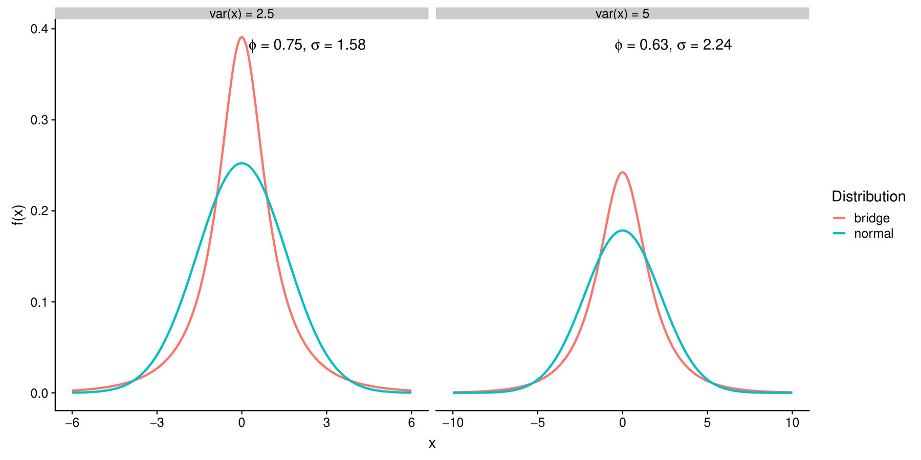 Figure 1
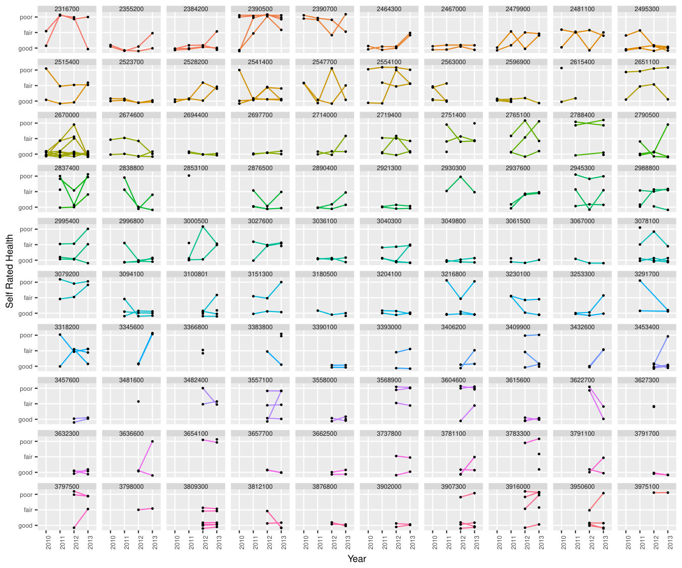 Figure 2
Peer Reviews
No public reviews on file for this paper yet. If you reviewed it on a platform where reviews are public (OpenReview, ICLR, NeurIPS, ICML), you can paste yours below so the community can read it here.
Videos
No videos yet. Explain this paper in a talk, walkthrough, or lecture? Add one.
\Author
Özgür Asar\Affil1 \AuthorRunningÖzgür Asar \Affiliations Department of Biostatistics and Medical Informatics, Faculty of Medicine, Acıbadem Mehmet Ali Aydınlar University, İstanbul, Turkey \CorrAddressÖzgür Asar, Department of Biostatistics and Medical Informatics, Faculty of Medicine, Acıbadem Mehmet Ali Aydınlar University, Kerem Aydınlar Kampüsü, Kayışdağı Cad., No: 32, Ataşehir, İstanbul, Turkey \[email protected] [email protected] \CorrPhone(+90) 216 500 4255 \CorrFax(+90) 216 576 5120 \TitleBayesian analysis of Turkish Income and Living Conditions data, using clustered longitudinal ordinal modelling with Bridge distributed random-effects \TitleRunningBayesian analysis of Turkish Income and Living Conditions data \Abstract This paper is motivated by the panel surveys, called Statistics on Income and Living Conditions (SILC), conducted annually on (randomly selected) country-representative households to monitor EU 2020 aims on poverty reduction. We particularly consider the surveys conducted in Turkey within the scope of integration to the EU. Our main interests are on health aspects of economic and living conditions. The outcome is self-reported health that is clustered longitudinal ordinal, since repeated measures of it are nested within individuals and individuals are nested within families. Economic and living conditions were measured through a number of individual- and family-level explanatory variables. The questions of interest are on the marginal relationships between the outcome and covariates that we address using a polytomous logistic regression with Bridge distributed random-effects. This choice of distribution allows us to directly obtain marginal inferences in the presence of random-effects. Widely used Normal distribution is also considered as the random-effects distribution. Samples from the joint posterior densities of parameters and random-effects are drawn using Markov Chain Monte Carlo. Interesting findings from public health point of view are that differences were found between sub-groups of employment status, income level and panel year in terms of odds of reporting better health.
\Keywords Bridge distribution; latent variables; multi-level data; repeated measures; self-reported health
1 Introduction
Statistics on Income and Living Conditions (SILC) are panel surveys that have been conducted in 28 EU and 4 non-EU countries (Turkey, Iceland, Switzerland and Norway) to monitor EU 2020 strategies on poverty reduction. In SILC, households are followed annually. Detailed information on income, poverty, social exclusion, living conditions, housing, labour, education and health are collected by questionnaires. The countries are not expected to use the same questionnaires. They can do modifications on the main questionnaire based on local conditions as long as they collect the minimum information.
In SILC, main study units are households. Data from a single country has a three-level data structure, since repeated observations are nested within individuals and individuals are nested within families. This kind of structure can also be called as clustered longitudinal. Income and living conditions have been measured through a number of individual- and family-level variables, e.g. mean household disposable income, gender, marital status, age, education level and working status. Health status is measured through self-reported health (SRH): individuals’ rate to the question, “How is your health in general?”. The rates can be one of the followings: very bad, bad, fair, good, and very good. SRH is an important indicator of individuals’ general health and argued to be a good predictor of morbidity and mortality (Burström and Fredlund, 2001).
In the current study, we are interested in exploring the relationships between health status and income and living conditions. We obtained data from the Turkish SILC (TR-SILC). It has been conducted by Turkish Statistical Institute (TURKSTAT) within the scope of European Union Statistics on Income and Living Conditions (EU-SILC). There are a number of papers that analysed EU-SILC data, excluding TR-SILC. To the best of our knowledge, there is no work that analysed panels from TR-SILC. Detailed literature review on SILC is provided in Section 3. None of the works considered drawing marginal inference (to be introduced below) with appropriate statistical modelling.
Our scientific questions are on the interpretations of the relationships between SRH and economic and demographic variables. Therefore, our first natural choice would be working with marginal models (Diggle et al., 2002, Chapter 8). For inferential purposes, generalised estimating equations (GEE; Liang and Zeger (1986)) could be used. However, this method does not work with a genuine likelihood function, and might not be the best option for unbalanced data. Instead, we consider random-effects models (Chapter 10 of Diggle et al. (2002)). This class of model consists of individual-level terms together with covariates. Interpretations of the regression coefficients are typically based on the assumption that two persons belonging to different covariate sub-groups have the same individual characteristics. However, this would be unrealistic in many cases. Wang and Louis (2003, 2004) invented a class of distribution, called Bridge distribution for logit link, that allows obtaining marginal interpretations for the covariates within the random-effects modelling framework. So far, the distribution is used only for binary data, mostly within the scope of analysis of longitudinal data, i.e. two-level data (Bandyopadhyay et al., 2010; Parzen et al., 2011; Tu et al., 2011; Li et al., 2011). Tom et al. (2015) used it for semi-continuous outcome data in the binary logistic sub-part model. Boehm et al. (2013) considered Bridge distribution for multi-level spatial binary data. In this study, we use Bridge distribution for analysis of three-level ordinal outcome data. We take the Bayesian paradigm for inference. The No-U-Turn Sampler (Hoffman and Gelman, 2014), an adaptive version of Hamiltonian Monte Carlo (Neal, 2011), is used to obtain samples from the joint posterior distributions of parameters and random-effects.
Rest of the paper is organised as follows. In Section 2, we give the details of TR-SILC data. In Section 3, we review the literature on both longitudinal ordinal modelling and analysis of SILC data. Section 4 presents model formulation and inferential details. Section 5 presents results on the TR-SILC data-set. We close the paper by conclusion and discussion.
2 TR-SILC Data-set
2.1 Background information
SILC surveys have been conducted in 28 EU countries and 4 non-EU countries (Turkey, Iceland, Switzerland and Norway) to monitor EU 2020 strategies on poverty reduction. The surveys cover objective and subjective questions on both monetary and non-monetary aspects of income, social inclusion and living conditions. Family- and individual-level micro-data are collected on income, poverty, social inclusion, living conditions, housing, labour, education and health. The surveys have been conducted as cross-sectionally and also as panels of four years. For more details, interested reader is referred to a data-resource paper on EU-SILC by Arora et al. (2015) and to the website of Eurostat at
http://ec.europa.eu/eurostat/web/income-and-living-conditions.
The surveys have been conducted in Turkey by TURKSTAT starting from 2006 within the scope of integration to the EU. Since then data have been collected annually as cross-sections and panels of four years. Country-representative families have been randomly selected, and those willing to participate have been included. Every year of the panels, new families (and individuals from these families), and/or new individuals, e.g. newborns, are included. If an individual leaves an existing family, and forms a new one, e.g. by getting married, the new family is also included in the study. For such a person, identity number is kept the same, and the new family is assigned a new identity number. More details regarding TR-SILC could be found at
http://www.turkstat.gov.tr/PreTablo.do?alt_id=1011.
2.2 Data-set
In the current study, we consider the panel of 2010 – 2013. Subjects who are older than 16 (inclusive) are considered, since SRH is not available for those who are younger than 16. There are a total of 109 066 records in the available data-set. Summary statistics on number of records, and family-level variables are displayed in Table 1, whereas summary statistics on individual-level variables are displayed in Table 2. Every year, new families and individuals were recruited to the panel. For example, whilst there were 3 056 families (8 090 individuals) available at 2010, there were 8 712 families (23 391 individuals) at 2011. The changes in the proportions for sub-groups of family size, gender, marital status, age, education level and working status were less than a per cent across successive years. Mean household disposable income (MHDI) is calculated by dividing household disposable income by family size. Note that although we report categorised family size in Table 1, original family sizes were used for MHDI calculation. MHDI was increasing through years, e.g. the medians were 6 614, 7 061, 7 757 and 8 586 Turkish Lira for 2010, 2011, 2012 and 2013, respectively. Clearly the variable is right-skewed, hence log-transformation will be applied when it is considered as an explanatory variable in a statistical model.
Follow-up patterns for families and individuals are displayed in Table 3. As can be seen, majority of the families and individuals were present at 2012–2013, 2011–2012–2013 and 2010–2011–2012–2013. There were 465 families and corresponding 2 515 individuals who were only present at 2013. The rest corresponds to either drop-out or intermittent missingness patterns, with 259 families and 873 individuals being in the latter pattern. If an individual is available at a follow-up, there is no missing data for her/him regarding the variables reported in Tables 1 & 2. One might argue that missing-at-random assumption (Little and Rubin, 2002) would be reasonable for the intermittent and drop-out patterns, since reasons for missing data include moving to another country, moving to nursing home, serving for the army, and so on. Likelihood-based inference would be reliable under this assumption (Diggle et al., 2002).
We consider re-categorising SRH as good health (composed of good and very good), fair health and poor health (composed of bad and very bad) (Abebe et al., 2016; Yardim and Uner, 2018). The percentage of people who reported good (bad) health were increasing (decreasing) through 2010–2013. There seems no clear pattern for fair health. Spagetti-plots of SRH data for a random sample of 100 families are displayed in Figure 1. In total, 699 repeated measures on 284 individuals from these families are displayed. The plots indicate that there are heterogeneities both between families and between individuals in terms of health status evolutions.
3 Literature Review
3.1 Modelling approaches for longitudinal ordinal data
In this sub-section, we review papers that propose modelling approaches for longitudinal ordinal data. We selected papers that cover a wide range of approaches to the topic. We first review papers on longitudinal (two-level), then clustered longitudinal (three-level) outcome.
Kosorok and Chao (1996) considered modelling ordinal data in continuous time by letting the intensity matrix being modified by explanatory variables. Maximum likelihood (ML) was considered for inference. Cowles et al. (1996) considered a tobit regression with random-effects and used Gibbs sampling to sample from the posterior densities. Varin and Czado (2010) considered a polytomous probit regression with a time-varying random-intercept that has an exponential correlation structure. Parameters were estimated by a pseudo-likelihood approach. Kaciroti et al. (2006) considered a polytomous logistic regression with both random-effects and transition terms within the context of non-ignorable missing data. They used Bayesian methods for inference. Bürgin and Ritschard (2015) proposed a mixed-effects polytomous regression with tree-based varying coefficients to take into account moderation of the covariate effects. ML was used for inference and the R package vcrpart (Bürgin and Ritschard, 2017) implements the proposed methodology. Pulkstenis et al. (2001) considered a mixed-effects model with log-log link and log-Gamma distributed random variables that is coupled with a discrete survival model. ML was used for inference. Laffont et al. (2014) considered a probit random-effects model for multivariate longitudinal ordinal data. Stochastic expectation-maximisation was considered for inference. Cheon et al. (2014) considered pattern-mixture type models with transition terms and estimated the parameters using ML. Kauermann (2000) considered a marginal polytoumous logistic regression with time-varying regression thresholds and covariate effects. Estimation was carried out by a method called local estimation. Jacqmin-Gadda et al. (2010) proposed a polytomous regression with time-independent and time-dependent random-effects with a smooth threshold term. Penalised likelihood was used for inference.
Lesaffre et al. (1996), Molenberghs et al. (1997) and van Steen et al. (2001) considered marginal modelling of longitudinal ordinal data with the multivariate Dale model that is coupled with a logistic regression to take into account non-ignorable drop-out. The authors used ML was for inference. Heagerty and Zeger (1996) developed a modelling framework that consists of two sub-models, a marginal polytomous regression for the covariate effects and a global odds-ratio model for pairwise association. GEE was considered for inference. Chen et al. (2014) extended their method to mis-classified response and covariate data. Ekholm et al. (2003) considered a polytomous marginal logistic regression with dependence ratios and used ML for inference. Perin et al (2014) considered a marginal polytomous regression and used GEE with orthogonalised residuals for parameter estimation. Zaloumis et al. (2015) considered a marginal polytomous regression with a non-proportional odds assumption based on a multivariate logistic distribution constructed by multivariate copula. Bayesian methods were used for inference. Nooraee et al. (2016) considered a similar approach by approximating logistic distribution by distribution with 8 degrees-of-freedom and used ML for inference.
Lee and Daniels (2007) and Lee and Daniels (2008) considered marginalised transition and random-effects models for analysis of longitudinal ordinal data, respectively. Lee et al (2013) extended the marginalised random-effects models to longitudinal bivariate ordinal outcomes. Lee et al. (2016) combined the transition and random-effects terms in the marginalised modelling framework in order to take into account long series of repeated measures. All of these four works considered ML for inference. Rana et al (2018) extended the work of Lee and Daniels (2008) to missing data and mis-reporting scenarios.
Raman and Hedeker (2005) and Chan et al. (2015) considered polytomous logistic regression modelling with random-effects for three-level ordinal outcomes. Liu and Hedeker (2006) considered a three-level polytomous logistic regression for longitudinal multivariate outcomes within the item-response theory framework. These works used ML for inference.
3.2 Analysis of SILC data
In this sub-section, we review the literature on analysis of SILC data mainly from the statistical analysis point of view. We found no work that considered analysis of SRH or any panel aspect of the TR-SILC data. The works that considered TR-SILC data are the followings. Oguz-Alper and Berger (2015) derived variance estimators for change in poverty rates using 2007 and 2008 cross-sections. Erus et al. (2015) investigated take-up of means-tested health benefits using 2007 cross-section. Yardim and Uner (2018) considered unmet access to healthcare based on 2006 and 2013 cross-sections using separate multinomial logistic regressions. Therefore, we review in detail only the works that considered analysis of the EU-SILC data. In the papers reviewed, generally statistical terminology is unclear and confusing. We decided to exclude the papers with limited information on statistical methods. None of the works considered marginal inference in the presence of random-effects. Marginal inferences are based on fixed-effects models that ignore dependency due to the nested structure of the data which is known to produce incorrect uncertainty quantification.
van der Wel et al. (2011) considered impacts of sickness dimension of health on employment status using a cross-section of data (year 2005) from 25 EU countries plus Norway and Iceland. The authors used a mixed model for two-level binary outcome (employed vs. unemployed) with a country-level random intercept. Reeves et al. (2014) also considered the impacts of sickness dimension of health on employment status, in the presence of the 2008 recession. 2006–2010 panel was divided into two: 2006–2008 (pre-recession) and 2008–2010 (during recession). Individual-level random intercepts (ignoring family- and country-level characteristics) were included in a mixed model for binary outcome. Ferraini et al. (2014) inspected the impacts of unemployment insurance on dichotomised SRH in 23 EU countries between 2006–2009, using a binary mixed model with individual-level random intercept. Barlow et al. (2015) investigated through logistic regression the impacts of austerity measures on SRH after the Recession using the 2008–2011 Greek SILC data. Vaalavuo (2016) considered the impacts of unemployment and poverty on deterioration in SRH from 26 EU countries using logistic regression. Pirani and Salvini (2015) inspected differences in health between temporary and permanent contract working classes using the 2007–2010 Italian SILC data. The outcome is dichotomised SRH and a marginal structural model was used. Huijts et al. (2015) inspected the impacts of job loss during the Recession using the 2009 EU-SILC data. The authors used a linear mixed model for dichotomised health with a country-level random intercept. Heggebø (2015) inspected the effects of health conditions on job loss during the Recession using the 2007–2010 Scandinavian SILC data. A linear mixed model with a individual-level random intercept was used. Tøge and Blekesaune (2015) analysed the 2008–2011 EU-SILC data to understand the impacts of job loss on health. They used a linear model for five-level SRH. Hessel (2016) considered the impacts of retirement on health using the 2009–2012 EU-SILC data. The model was a linear mixed model with a individual-level random intercept. Tøge (2016) considered the impacts of unemployment on SRH using the 2008–2011 EU-SILC data. A linear mixed model with a subject-specific random intercept was used. Abebe et al. (2016) inspected the impacts of the Recession using the 2005–2011 EU-SILC data. The authors used a mixed effects logistic model for three-level SRH. Giannoni et al. (2016) considered migrant health policies and health inequalities using the 2012 EU-SILC data. Ordinal SRH outcome was analysed using a country-level random-intercept in a polytomous regression. Clair et al. (2016) investigated the impacts of housing payment problems on health using the 2008–2010 EU-SILC data. Dichotomised SRH was analysed using a linear mixed effects model with subject-, household- and country-level random-effects. This is the only work that considered family-level heterogeneity. Bacci et al. (2017) considered the 2009–2012 EU-SILC for investigating impacts of economic deprivation on SRH, using a subject-specific random intercept in a polytomous logistic regression for ordinal SRH.
4 Modelling framework
4.1 Formulation
Let denote an ordinal response with possible values, i.e. , for subject belonging to family at follow-up at time . Also let denote the covariate matrix ( dimensional) attached to each of . There are repeated measures for family , and follow-ups in total.
For TR-SILC, the target of inference is on the relationships between covariates and ordinal reponses, i.e. on the conditional distribution of , where “” stands for “the distribution of”, and are marginal parameters in the sense that the relationship between covariates and responses are not conditioned on other terms, e.g. response history and/or individual characteristics. A regression modelling framework for this distribution would be
[TABLE]
where is a link function, and is a function that relates the covariates and associated coefficients to the probability of ordinal outcome taking the value , . Choices of cumulative logit for and linear regression for would yield the following polytomous logistic regression:
[TABLE]
Here, is the category-specific intercept, also known as the threshold, are the regression coefficients. address the target of inference for TR-SILC. The issue with this model is that full-likelihood based inference is not easy, since specification of the joint distribution of , where , a multivariate multinomial distribution with complex dependence structures, is not straightforward in practice. In order for likelihood based inference, one can include random-effects in (2) such that
[TABLE]
where denotes the random-effect, also known as latent-effect, for individual belonging to family at the follow-up at time . Note that is unobserved, and typically a distribution is postulated to it. The superscript in (3) stands for the related terms being conditional on . The regression coefficients that address the target of inference, , typically cannot be directly obtained from (3) due to logit link.
4.2 Random-effects specifications
A special, albeit useful approach would be to de-compose the random effect term as , where (Raman and Hedeker, 2005; Chan et al., 2015). This approach is also useful to take into account individuals in TR-SILC who forms a new family but still included in the survey. For such a patient, term would change, i.e. family characteristic would change, but would stay the same. Assuming time-independent random intercept terms, i.e. absence of the index in and would be sufficient to capture dependence for data-sets with a few repeats per study-units. Note that for TR-SILC majority of the families include at most five individuals (see Table 1) and maximum number of repeats per family/subject is four, and there are many individuals with less than four repeats (see Table 3).
The relationships between and , and and , would be available through solving the following convolution equation:
[TABLE]
where are the random-effects parameters. The relationships are not available in closed-form for the widely used random-effects distributions, e.g. Normal distribution, due to the logit link. Using Bridge distributional assumptions one can obtain the analytical relationship as follows. If one considers , where , and , with , then, the marginal estimates are available analytically as and (Wang and Louis, 2003; Boehm et al., 2013). For the concept of bridging, one can see Kenward and Molenbergs (2016). Note that the distribution of is no longer Bridge; we call it Modified Bridge. Density functions of the Bridge and Modified Bridge are given in Appendix A. Both distributions are symmetric and zero-mean. Under Bridge, is zero-mean, and has a variance of . Under Modified Bridge, is zero-mean and has a variance of . Bridge density is plotted in Figure 2 against Normal for two settings of variance.
We also consider Normal distribution for the random-effects: and . Note that the model with Normal random-effects corresponds to the models considered in Raman and Hedeker (2005) and Chan et al. (2015).
4.3 Bayesian Inference
Let’s denote the responses in the data-set by , where and . Also let’s denote the covariates by , where , (with as before), with being an operator that stacks the matrices on bottom of each other.
The joint posterior distribution of the parameters, , where , and , and random effects, , where , where and given data, and , is given by
[TABLE]
By assuming random-effects and associated parameters are independent of the covariates, the joint posterior (5) can be re-written as
[TABLE]
Here, is the likelihood:
[TABLE]
In (7), is multinomial distribution such that
[TABLE]
with to be obtained from (3).
By specifying , with , one would obtain as
[TABLE]
For Bridge random-effects, , , , , and . For Normal, , , , . Note that for Normal, .
Weakly informative priors are specified for the parameters. For and , we consider Cauchy priors with location parameter 0 and scale parameter 5 (Gelman et al., 2008). Standard deviations of the distributions, e.g. for for Bridge, are assigned half-Cauchy with location 0 and scale 5 (Gelman, 2006; Polson and Scott, 2012).
Samples from the joint posterior density are drawn using The No-U-Turn Sampler of Hoffman and Gelman (2014), a modified version of Hamiltonian Monte Carlo (Neal, 2011), as implemented in Stan (Carpenter et al., 2017). Computations were carried out in R (r2018) using bespoke code that relies on the rstan package (Stan Development Team, 2018). Bespoke R codes, a simulated data-set, and exemplary codes for data analysis are available in the R package mixed3 (https://github.com/ozgurasarstat/mixed3).
5 Application: TR-SILC data-set
5.1 Results
As mentioned in Section 2, the outcome variable is re-categorised SRH with three levels (): good health (), fair health (), and poor health (). Explanatory variables are listed in Tables 1 & 2.
We fit to the TR-SILC data-set the three-level models with Modified Bridge distributed and Bridge distributed (Modified Bridge - Bridge model), and Normally distributed and Normally distributed (Normal - Normal model). We also fit the two-level mixed model with Bridge distributed by dropping from the model (two-level Bridge model), and the fixed-effects model by dropping both and . For all the four models, we specifically consider proportional odds assumption, i.e. , as there are fairly many explanatory variables. For each model, four chains of length 2,000 were run in parallel starting from random initials. First halves of the chains were treated as the warm-up period. Trace-plots, density plots and R-hat statistics (Brooks and Gelman, 1997) were used to assess convergence. Fitting each of the three-level models took around ten hours, whereas it took around nine hours for the two-level model and around an hour the fixed-effects model, on a 64 bit desktop computer with 16,00 GB RAM and AMD Ryzen 7 1800X Eight Core Processor 3.60 GHz running Windows 10.
We consider the Watanebe information criterion (WIC; Watanebe (2010), Gelman et al. (2014)) and log pseudo marginal likelihood (LPML; Dey et al (1997), Gelman et al. (2014)) for model comparison. The formulae that we used to calculate these criteria are given in Appendix B. Lower values of WIC and higher values of LPML indicate better fit. Table 4 displays the values obtained for the models used to analyse the TR-SILC data-set. Both WAIC and LPML indicate that the Modified Bridge - Bridge model is the best fitting model. Normal - Normal model is the second, two-level Bridge is the third and the fixed-effects model is the fourth model.
Conditional results are presented in Table 6, whereas marginal results are presented in Table 7. With regards the conditional results, , different random-effects distributional assumptions for three-level models produced similar results. This would be expected, since all the distributions are zero-mean and symmetric. In addition, this would be considered as a good sign, because Modified Bridge - Bridge pair can be used instead of the widely used Normal distribution, and the pair brings the advantage of direct marginal inferences as discussed in Section 4.2. The two-level Bridge model also produced similar results up to some extent. With regards marginal results, , Modified Bridge - Bridge and two-level Bridge models again produced similar results. There are considerable differences between these two models and the fixed-effects model. For example, for “Students”, whilst the 95% credibility interval is (-0.242, -0.035) under the Modified Bridge - Bridge model, it is (-0.418, -0.211) under the fixed-effects model.
Interpretations under the preferred model (Modified Bridge - Bridge model) are as follows. Females were approximately 29% more likely to report worse health compared to males. Widowed or separated (never married) people were more (less) likely to report worse health compared to married people. People in the 35 – 64 (65+) age group were less (more) likely to report worse health compared to those in the 16 – 34 age group. Higher education level was associated with decreased probability of reporting worse health. Except students, all the other working status categories were more likely to report worse health compared to those working full or part time. Unemployed people were approximately 22% more likely to report worse health compared to the full or part time working people. MHDI is inversely associated with SRH such that 1% decrease in MHDI level was associated with approximately 32% increased odds of reporting worse health. Odds of reporting worse health did not change in year 2011 compared to 2010; the credibility interval for is (-0.082, 0.011). On the other hand, in 2012 and 2013 people were less likely to report worse health compared to 2010. They were approximately 12% (9%) more likely to report worse health in 2010 compared to 2012 (2013).
5.2 Posterior predictive checks
We performed posterior predictive checks to see how the replicated data based on the fitted models match the observed data. For this, we simulated data from
[TABLE]
for the Modified Bridge - Bridge, Normal - Normal and the two-level Bridge models, and from
[TABLE]
for the fixed-effects model, for each of the 4 000 elements of the MCMC samples. Each of the 4 000 simulated data-sets were then compared with the observed data. We calculated percentages of matches and mis-matches between the observed and replicated data-sets. Means and standard deviations of the percentages are displayed in Table 5. In this table, “-2” means observed outcome being “good health” and replicated being “poor health”; “-1” means observed being “good health” and replicated being “fair health”, or observed being “fair health” and replicated being “poor health”; “0” means observed and replicated being the same; “1” means observed being “fair health” and replicated being “good health”, or observed being “poor health” and replicated being “fair health”; “2” means observed being “poor health” and replicated being “good health”. In summary, non-zero values mean mis-match between the observed and replicated data-sets, whilst “-2” and “2” would mean the most difference between the two. Modified Bridge - Bridge, Normal-Normal and two-level Bridge models seem to be perform similarly in terms of replicating the observed data. Fixed-effects model seems to be the worst amongst the four models, as its mean percentage for “0” is lower and mean percentages for “-2” and “2” are higher compared to the other models.
6 Conclusion and Discussion
In this paper, we presented an analysis of Turkish Income and Living Conditions data, with the perspective of marginal inference on the relationships between the outcome and explanatory variables. The outcome of interest is ordinal taking three values: good, fair and bad health. It is subject to family- and individual-level dependencies. In other words, it is three-level or clustered longitudinal. The model we consider is cumulative logistic regression. We introduced random-effects in order for likelihood-based inference. Typically the estimates obtained under the random-effects models have conditional interpretations, hence do not address the scientific interests of the current work. Bridge distributional assumptions for the random-effects allows one to obtain marginal inferences analytically. We take a Bayesian perspective for inference. Samples from the joint posterior distributions are drawn using an adaptive Hamiltonian Monte Carlo algorithm, called the No-U-Turn Sampler. The R package mixed3 contains functions that implement the methods in practice.
The findings regarding working status, MHDI and panel years are important from the public health point of view. The difference between employed and unemployed people in terms of reporting better health emphasises the importance of reducing unemployment rate. Inverse association between MDHI levels and probability of reporting better health points out the vitality of economic conditions to reaching better healthcare. Differences in cohort years are important to understand the impacts of changes in health policies.
In the panels of TR-SILC, neither geographical nor urban/rural information was available. These information would explain some source of variation in SRH. Mediation analysis would be interesting. For example, education level would effect income and hence health status. Cumulative and/or lagged effects of explanatory variables might be considered to explain health status. For example, history of unemployment might be predictor of current health status. We leave these to a future work on substantive analysis of TR-SILC. Marginalised models (Lee and Daniels, 2007) could be extended to three-level ordinal outcomes. However, the estimation procedure would be computationally more demanding compared to the present approach, as one needs to solve intractable convolution equations through root finding algorithms, e.g. Newton-Raphson. Currently we do have access only to TR-SILC. It would be interesting if we were able to add EU and other SILC data into our analysis. In such a case, the data would be four-level due to the additional nested structure of families being nested within countries. It would be interesting to explore Bridge random-effects specification for four-level ordinal outcomes. From practical point of view, however, one can include countries as dummy variables in the design matrix, as there will be 32 countries.
Acknowledgements
The author thanks to Dr. Mahmut Yardım (Hacettepe University) for bringing the TR-SILC data-set into his attention and helpful discussions, Prof. Peter Diggle (Lancaster University) for helpful comments on a draft, Dr. Jonas Wallin (Lund University) and Dr. David Bolin (University of Gothenburg and Chalmers University of Technology) for helpful discussions on modelling and inference, and TURKSTAT for making the data available. The views expressed in this paper are those of the author.
Appendix A Density functions
The density function of Bridge distribution for logit link is given by
[TABLE]
where is the hyperbolic cosine, defined as . Bridge distribution is symmetric, zero-mean and has a variance of . The density function of modified Bridge, for generic , and with , , , is given by
[TABLE]
Modified Bridge is zero-mean, and has a variance of .
Appendix B Model selection
WAIC is calculated as
[TABLE]
where, “lppd” stands for log pointwise posterior density and is calculated as
[TABLE]
and is the effective number of parameters and calculated as
[TABLE]
with
[TABLE]
In (15) - (17), , and denote th draw of and , from the joint posterior densities.
Conditional predictive ordinate (CPO) is defined as leave-one-out cross-validated predictive density, such that , where is the without observation . The harmonic mean estimate of CPO, as proposed by Dey et al (1997), is
[TABLE]
LPML is then defined as
[TABLE]
The reference list from the paper itself. Each links out to its DOI / PubMed record.
- 1Abebe et al. (2016) Abebe, D. S., Tøge, A. G., and Dahl, E. (2016). Individual-level changes in self-rated health before and during the economic crisis in Europe. International Journal for Equity in Health , 15(1) , 1–8.
- 2Arora et al. (2015) Arora, V. S., Karanikolos, M., Clair, A., Reeves, A., Stuckler, D., and Mc Kee, M. (2015). Data Resource Profile: The European Union Statistics on Income and Living Conditions (EU-SILC). International Journal of Epidemiology , 44(2) , 451–461.
- 3Bacci et al. (2017) Bacci, S., Pigini, C., Seracini, M., and Minelli, L. (2017). Employment condition, economic deprivation and self-evaluated health in Europe: Evidence from EU-SILC 2009–2012. International Journal of Environmental Research and Public Health , 14:143 , doi.org/10.3390/ijerph 14020143.
- 4Barlow et al. (2015) Barlow, P., Reeves, A., Mc Kee, M., and Stuckler, D. (2015). Austerity, precariousness, and the health status of Greek labour market participants: Retrospective cohort analysis of employed and unemployed persons in 2008–2009 and 2010–2011. Journal of Public Health Policy , 36(4) , 452–468.
- 5Boehm et al. (2013) Boehm, L., Reich, B. J., and Bandyopadhyay, D. (2013). Bridging Conditional and Marginal Inference for Spatially Referenced Binary Data. Biometrics , 69 , 545–554.
- 6Bandyopadhyay et al. (2010) Bandyopadhyay, D., Sinha, D., Lipsitz, S., and Letourneau, E. (2010). Changing approaches of prosecutors towards juvenile repeated sex-offenders: A Bayesian evaluation. The Annals of Applied Statistics , 4(2) , 805–829.
- 7Brooks and Gelman (1997) Brooks, S. P., and Gelman, A. (1997). General methods for monitoring convergence of iterative simulations. Journal of Computational and Graphical Statistics , 7 , 434–455.
- 8Bürgin and Ritschard (2015) Bürgin, R., and Ritschard G. (2015). Tree-based varying coefficient regression for longitudinal ordinal responses. Computational Statistics and Data Analysis , 86 , 65–80.