PDE eigenvalue iterations with applications in two-dimensional photonic crystals
Robert Altmann, Marine Froidevaux

TL;DR
This paper develops iterative methods for solving PDE eigenvalue problems in 2D photonic crystals, including nonlinear cases, demonstrating convergence and efficiency improvements through adaptive refinement and Newton-type iterations.
Contribution
It extends classical eigenvalue algorithms to infinite-dimensional PDE problems and introduces a Newton method for nonlinear eigenproblems in photonic crystal modeling.
Findings
Inverse power method converges on operator level.
Adaptive mesh refinement accelerates computations.
Newton-type iteration achieves local quadratic convergence.
Abstract
We consider PDE eigenvalue problems as they occur in two-dimensional photonic crystal modeling. If the permittivity of the material is frequency-dependent, then the eigenvalue problem becomes nonlinear. In the lossless case, linearization techniques allow an equivalent reformulation as an extended but linear and Hermitian eigenvalue problem, which satisfies a Garding inequality. For this, known iterative schemes for the matrix case such as the inverse power or the Arnoldi method are extended to the infinite-dimensional case. We prove convergence of the inverse power method on operator level and consider its combination with adaptive mesh refinement, leading to substantial computational speed-ups. For more general photonic crystals, which are described by the Drude-Lorentz model, we propose the direct application of a Newton-type iteration. Assuming some a priori knowledge on the…
Click any figure to enlarge with its caption.
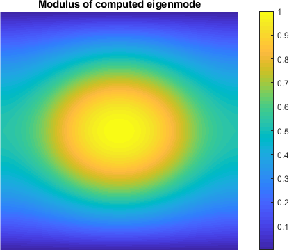 Figure 1
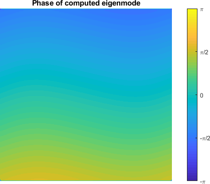 Figure 2
| on fine mesh | steps per mesh | steps per mesh | steps per mesh |
|---|---|---|---|
| 129.136 | 72.396 | 46.585 | 42.308 |
| on fine mesh | steps per mesh | steps per mesh | steps per mesh |
|---|---|---|---|
| 100.56 | 71.96 | 51.39 | 34.49 |
| 1 | 2 | 3 | 4 | 5 | 6 | 7 | |
|---|---|---|---|---|---|---|---|
| 416.6166 | 352.7054 | -339.9124 | 492.5687 | -19.6143 | -527.5597 | 98.0101 | |
| 92.1086 | 71.6269 | 71.4552 | 227.8301 | 47.4923 | 93.5605 | 121.3762 | |
| 2.7820 | 0.9597 | 0.9500 | 13.1508 | 9.2697 | 3.2624 | 2.2712 |
Peer Reviews
No public reviews on file for this paper yet. If you reviewed it on a platform where reviews are public (OpenReview, ICLR, NeurIPS, ICML), you can paste yours below so the community can read it here.
Videos
No videos yet. Explain this paper in a talk, walkthrough, or lecture? Add one.
PDE Eigenvalue Iterations with Applications in
Two-dimensional Photonic Crystals∗
R. Altmann†, M. Froidevaux*‡*
† Institut für Mathematik, Universität Augsburg, Universitätsstr. 14, 86159 Augsburg, Germany
‡ Institut für Mathematik MA4-5, Technische Universität Berlin, Straße des 17. Juni 136, 10623 Berlin, Germany
[email protected], [email protected]
Abstract.
We consider PDE eigenvalue problems as they occur in two-dimensional photonic crystal modeling. If the permittivity of the material is frequency-dependent, then the eigenvalue problem becomes nonlinear. In the lossless case, linearization techniques allow an equivalent reformulation as an extended but linear and Hermitian eigenvalue problem, which satisfies a Gårding inequality. For this, known iterative schemes for the matrix case such as the inverse power or the Arnoldi method are extended to the infinite-dimensional case. We prove convergence of the inverse power method on operator level and consider its combination with adaptive mesh refinement, leading to substantial computational speed-ups. For more general photonic crystals, which are described by the Drude-Lorentz model, we propose the direct application of a Newton-type iteration. Assuming some a priori knowledge on the eigenpair of interest, we prove local quadratic convergence of the method. Finally, numerical experiments confirm the theoretical findings of the paper.
∗ Research funded by the Einstein Foundation Berlin in the frame of Einstein Center for Mathematics Berlin ECMath via project OT10 Model Reduction for Nonlinear Parameter-Dependent Eigenvalue Problems in Photonic Crystals and by the Deutsche Forschungsgemeinschaft (DFG, German Research Foundation) under Germany’s Excellence Strategy – The Berlin Mathematics Research Center MATH+ (EXC-2046/1, project ID: 390685689).
**Key words. nonlinear eigenvalue problem, photonic crystals, inverse power method, Newton iteration
AMS subject classifications. 65N25, 65J10, 65F15**
1. Introduction
Eigenvalue problems including partial differential equations (PDE) appear in several applications such as structural mechanics [BW73], fluid-solid structures [Vos03], or the simulation of Bose-Einstein condensates [PS03]. In general, such problems are considered in order to optimize certain properties or parameters of the underlying dynamical system [MV04]. In this paper, we focus on applications as they appear in the modeling of photonic crystals [Joh87, Kuc01]. These are special composite materials with a periodic structure that affect the propagation of electromagnetic waves and thus, can be used for trapping and guiding light. As these crystals can be designed and manufactured for industrial applications, the aim is to find so-called photonic band-gaps, which prevent light within a specified frequency range from propagating [JJWM08, Joh12]. Direct applications areas are optical fibers [GH14, Ch. 5], medical technologies with laser guides for cancer surgeries [Tsa12], and thin film solar cells [DJ12].
The corresponding mathematical model is given by a sequence of nonlinear PDE eigenvalue problems based on the Maxwell equations [SP05, DLP*+*11]. An important role is played by the electric permittivity , which is periodic in space and characterizes certain properties of the crystal. If is independent of the frequency, then we obtain a linear eigenvalue problem. In more realistic models, however, the permittivity is approximated by a rational function, which introduces the nonlinearity into the eigenvalue problem.
Numerical methods for computing the spectrum of such materials have been studied intensively. This includes adaptive finite element methods [BKS*+*06, GG12], Newton-type methods [Kre09, HLM16], and linearization techniques [SB11, EKE12]. In the latter case, a spatial discretization is assumed and yields then a linear but extended eigenvalue problem, for which well-known iteration schemes can be applied. The combination of mesh refinement and (inexact) eigenvalue iteration methods has been considered in [MM11, Mie11].
Corresponding iterative methods for the operator case have, so far, not received much attention in the literature. In the first part of this paper, we focus on linear and Hermitian PDE eigenvalue problems in the weak formulation. This corresponds to the case of a frequency-independent permittivity. Convergence of the (inverse) power method for compact operators mapping from a Hilbert space to was already shown in [ESL95]. In this setting, the proof basically follows the same lines as in the finite-dimensional case. General bounded operators were considered in [EE07] but only together with a power iteration based on the exact (und thus unknown) eigenvalue. Considering the weak formulation, which is more natural in view of spatial discretization methods, we are in a different setting. Nevertheless, the power method converges if an appropriate scaling is included. For the -Laplacian eigenvalue problem, this was shown in [Boz16]. Note that the proven convergence on operator level has the advantage that it is mesh- and basis-independent, cf. [AHP19] for a similar approach applied to nonlinear eigenvector problems. Thus, dependencies on a particular discretization do not play a role. Further, the approach allows to choose the spatial discretization in each iteration step independently.
The second part of the paper focuses on the nonlinear case as it appears in two-dimensional photonic crystal modeling. Here we consider two different paths of either linearizing the problem or applying directly a Newton iteration. In the first case, we adapt the techniques introduced in [SB11, EKE12] in combination with an inverse power iteration applied to the resulting linear problem. Due to the linearization, certain compactness properties get lost, which calls for a novel convergence analysis for the inverse power method. The second strategy translates the local convergence of Newton’s method from [Sch08] to the operator case. An analogous method for infinite-dimensional eigenvalue problems was developed in [AR68], and its local convergence was proven for Fredholm operators with index [math] mapping from a Hilbert space to . We show a similar result when the operators arise from the here considered weak formulation.
The paper is structured as follows. In Section 2 we introduce the problem setting, i.e., the linear PDE eigenvalue problem in its weak and operator formulation. Here we gather all the assumptions on the spaces and included operators. In particular, we assume an underlying Gelfand triple with a compact embedding. Section 3 then considers several iteration schemes including the inverse power method and the Arnoldi method. Two-dimensional photonic crystals with frequency-dependent permittivity are then topic of Sections 4 and 5. First, we consider a special Hermitian case. For this, we apply a linearization and the inverse power method. More realistic models are then discussed in Section 5, for which we prove the local convergence of Newton’s method. Finally, we present three numerical examples in Section 6.
2. Preliminaries
As described in the introduction, we consider the weak formulation of a PDE eigenvalue problem. Given the sesquilinear forms and , we search for a non-trivial pair such that for all test functions it holds that
[TABLE]
More precisely, considering Hermitian eigenvalue problems, we are interested in the eigenpair corresponding to the smallest eigenvalue. In the following, we gather assumptions on the space and the included sesquilinear forms. Afterwards we discuss well-known PDE eigenvalue problems, which fit into the given framework.
2.1. General setting
We start with general assumptions on the involved function spaces.
Assumption 2.1* (Function spaces).*
We assume to be a complex, separable, and reflexive Banach space. Furthermore, we assume the existence of a complex and separable Hilbert space (the pivot space) such that , , form a Gelfand triple, cf. [Zei90, Ch. 23.4] and [Bre10, Ch. 11.4]. This means, in particular, that the embedding is continuous and dense [Wlo87, Ch. 17.1]. The continuity constant is denoted by .
Assumption 2.2* (Compactness).*
The embedding is compact.
With the pivot space in hand, we assume that the sesquilinear form in (2.1) is also defined for functions in . We even assume that this defines the inner product in the Hilbert space and set . Further, denotes the Riesz isomorphism. The norm in the space is denoted by . For the sesquilinear form we consider the following assumptions.
Assumption 2.3* (Sesquilinear form).*
The sesquilinear form is assumed to be continuous and Hermitian such that for all . Furthermore, satisfies a Gårding inequality, i.e.,
[TABLE]
for real constants , and all , see e.g. [QV94].
Remark 2.4*.*
The previous Assumption 2.3 implies that is -coercive and thus, defines an inner product in . As a result, is actually a Hilbert space and the corresponding norm
[TABLE]
the so-called energy norm, is equivalent to . Further, all eigenvalues of (2.1) satisfy , which implies and thus .
In order to be well-posed, an eigenvalue problem of the form (2.1) requires boundary conditions. Throughout this paper, we assume that these conditions are included in the space , cf. the examples in the following subsection. We close this preliminary part with the proof of Young’s inequality in the specific case of complex vectors.
Lemma 2.5** (Young’s inequality).**
Consider . Then, for every we have an estimate of the form
[TABLE]
where denotes the real dot product.
Proof.
For any two vectors , the following estimates hold:
[TABLE]
As a consequence, we have . The claim then follows by setting , and . ∎
2.2. Examples
We present a couple of well-known examples, which fit into the given framework if formulated in the weak setting.
Example 2.6** (Laplace eigenvalue problem).**
Consider the eigenvalue problem in a bounded domain with homogeneous Dirichlet boundary conditions. For this, we set with and with the standard inner product. The corresponding sesquilinear form reads . Note that this implies and thus, and . The weak form of the Laplace eigenvalue problem then reads: find a non-trivial pair such that for all it holds that
[TABLE]
Example 2.7** (Schrödinger eigenvalue problem).**
The computation of the ground state of the linear Schrödinger operator leads to the sesquilinear form
[TABLE]
with a real-valued potential . For homogeneous Dirichlet boundary conditions this leads to the same spaces and as in Example 2.6. Further, satisfies the Gårding inequality with and \beta=\max\big{\{}0,-\inf_{x\in\Omega}W(x)\big{\}}. For periodic boundary conditions one has to replace the space accordingly.
In this paper, we focus on applications with photonic crystals. The dynamics of the electromagnetic fields inside such a crystal can be modelled by the Maxwell equations in the whole domain , cf. [DLP*+*11, Ch. 1]. These equations combine the magnitudes of the time-harmonic electric and magnetic fields , and the frequency , which takes the role of an eigenvalue.
One crucial parameter within the equations is the relative electric permittivity of the materials inside the crystal. We assume the relative permittivity to be piecewise-constant and periodic in space as well as bounded in the sense that
[TABLE]
for all and in some frequency domain of interest. For the applications in mind, where is given as a rational function, this means that we consider bounded away from the poles. In the two-dimensional case, i.e., when is periodic within a two-dimensional plane and constant along the direction orthogonal to this plane, the Maxwell eigenvalue problem decouples into so-called transverse magnetic (TM) and transverse electric (TE) modes. Thanks to the periodicity of , which implies a discrete translational symmetry in the system, a Floquet transformation can be applied to reduce the problem posed in to a family of problems on a bounded domain called the Wigner–Seitz cell of the crystal lattice, see e.g. [Kuc01, DLP*+*11]. Note that the function is here a unitless quantity expressed relative to , the vacuum permittivity. Within this paper, we assume the magnetic permeability of the crystal to be constant and equal to that of vacuum denoted by .
Example 2.8** (TM mode).**
In the two-dimensional setting we consider the TM mode with a real-valued frequency-independent function . The resulting PDE eigenvalue problem describes the third component of the electric field , from which one can directly compute the components and . Let be a fixed wave vector in the so-called irreducible Brillouin zone , cf. [DLP*+*11, Ch. 1], be the Floquet transform of at , and denote the shifted gradient. Then, satisfies the eigenvalue problem
[TABLE]
for all . For the sake of conciseness, we use in the following by abuse of notation a scaled frequency defined by . For the weak formulation of the eigenvalue problem we then define . Including periodic boundary conditions, we set with the standard -norm and . Note that is densely embedded in and thus, Assumption 2.1 is satisfied, cf. [Bre10, Ch. 4.4]. The sesquilinear form and the (weighted) inner product in then read
[TABLE]
and
[TABLE]
Due to the boundedness of , the sesquilinear form defines an inner product in . The following lemma shows that satisfies Assumption 2.3.
Lemma 2.9**.**
For a fixed wave vector the sesquilinear form defined in (2.2) in Example 2.8 is Hermitian, continuous, and satisfies Gårding’s inequality for any .
Proof.
Clearly, the sesquilinear form is Hermitian. For the continuity we apply the Cauchy-Schwarz inequality with respect to the complex dot product in as well as the inner product in and obtain for all ,
[TABLE]
Young’s inequality from Lemma 2.5 with then yields
[TABLE]
which proves the continuity of . To show the Gårding inequality, we first consider the case . Then, for any , we have
[TABLE]
i.e., the Gårding inequality with . Otherwise, for , we apply once more Lemma 2.5 for some parameter and get
[TABLE]
Now assume and define . Then, satisfies the Gårding inequality with . Note that can be chosen arbitrarily small with an appropriate choice of . ∎
Example 2.10** (TE mode).**
In the eigenvalue problem corresponding to the TE mode, the relative permittivity appears in the differential operator. More precisely, for a fixed wave vector , we search for such that
[TABLE]
for all . Considering again periodic boundary conditions, we set and with the standard inner products. In this case, the sesquilinear form has the form
[TABLE]
The proof of the Gårding inequality follows similarly as in Lemma 2.9.
More general eigenvalue problems are discussed in Sections 4 and 5. There we consider a TM mode with an electric permittivity, which depends on the frequency . This then leads to a nonlinear eigenvalue problem.
2.3. Operator formulation
The weak formulation of the eigenvalue problem (2.1) can be equivalently written as an operator equation in the (conjugate) dual space of , i.e., the space of conjugate linear and continuous mappings from . This then yields a convenient formulation for the introduction of iterative schemes. We introduce the operator by
[TABLE]
Further, we define as the embedding of in induced by the Gelfand triple , , from Assumption 2.1 with respect to the inner product in , cf. [Zei90, Ch. 23.4]. To be precise, this means for all . The operator equation corresponding to (2.1) then reads
[TABLE]
Note that this equation is stated in the dual space of , which means that we consider test functions in as in (2.1). Hence, the two formulations (2.1) and (2.3) are equivalent.
Finally, recall the definition of the shifted sesquilinear form from Remark 2.4. With this, we define the corresponding operator , which is then positive and thus, invertible.
3. Iterative Methods on Operator Level
In this section, we analyze iterative methods to find the smallest eigenvalue as well as the corresponding eigenfunction of the operator eigenvalue problem (2.3). We emphasize that we do not apply any spatial discretization but perform the eigenvalue iteration directly to the operator equation.
We first consider the inverse power method for which we prove the convergence in under the assumptions collected in the previous section. For this we consider two variants of the method and discuss the commutativity of spatial discretization and eigenvalue iteration, assuming an appropriate normalization within the scheme. Second, we discuss Arnoldi’s method for the operator case, based on Krylov subspaces as in the matrix case.
3.1. Inverse power method
Power and inverse power methods come in various variants with different kinds of scaling, see e.g. [AK08, Ch. 10.3] or [Saa11, Ch. 4] for the matrix case. One may even consider the scaling with the exact eigenvalue as done, e.g., in [EE07, AHP18]. Clearly, the latter is only of interest for theoretical observations rather than actual computations.
As for every iteration scheme we assume a starting function . In order to permit the iterates to converge to the wanted eigenfunction, one needs an additional assumption on , e.g., having a non-vanishing component in the direction of this eigenfunction.
3.1.1. Rayleigh quotient iteration
A direct application of the inverse power method for the operator case would apply the inverse of the differential operator over and over again. However, this operator may not be invertible and the Rayleigh quotient is not guaranteed to remain positive. Thus, we consider the shifted eigenvalue problem
[TABLE]
This then leads to the following algorithm: Given an initial function , , we solve for the variational problem
[TABLE]
Therein, includes the normalization in , which is the natural norm corresponding to the eigenvalue problem (2.3). Further, denotes the Rayleigh quotient, i.e.,
[TABLE]
We emphasize that the iterates of the power iteration (3.2) are not normalized. The presence of the Rayleigh quotient within the iteration directly provides an approximation of the eigenvalue , given by . It remains to discuss the convergence of the suggested iteration.
Theorem 3.1**.**
Given Assumptions 2.1-2.3, the power iteration (3.2) converges to an eigenpair (u^{\scalebox{0.5}{\bigstar}},\lambda^{\scalebox{0.5}{\bigstar}}) of (2.3) in the sense that the (sub)sequences and satisfy u^{j}\rightarrow u^{\scalebox{0.5}{\bigstar}} in and \lambda^{j}\rightarrow\lambda^{\scalebox{0.5}{\bigstar}} with \mathcal{A}u^{\scalebox{0.5}{\bigstar}}=\lambda^{\scalebox{0.5}{\bigstar}}\mathcal{I}u^{\scalebox{0.5}{\bigstar}} in .
Proof.
We follow the proof in [Boz16] where the convergence of the inverse power method for the -Laplacian is shown. The first step is to show the monotonic decrease of the sequence . For this, we consider (3.2) with test functions and leading to
[TABLE]
A combination of these two estimates yields and thus,
[TABLE]
The monotonicity and , which follows from the positivity of , imply that there exists the limit \mu^{\scalebox{0.5}{\bigstar}}:=\lim_{j\to\infty}\mu^{j}\geq 0. It even holds \mu^{\scalebox{0.5}{\bigstar}}>0, since the are uniformly bounded away from zero.
As a second step, we conclude from estimate (3.3) that . Since the norms and are equivalent, we obtain that is uniformly bounded in . Thus, there exists a convergent subsequence and an element {\tilde{u}}^{\scalebox{0.5}{\bigstar}}\in\mathcal{V}, which satisfy (without relabeling)
[TABLE]
Note that we have used here the compact embedding from Assumption 2.2. Obviously, we have \|{\tilde{u}}^{\scalebox{0.5}{\bigstar}}\|=\lim_{j\to\infty}\|\tilde{u}^{j}\|=1. Further, we know from previous calculations that
[TABLE]
This means that the sequence is uniformly bounded in . Thus, there exists a limit u^{\scalebox{0.5}{\bigstar}}\in\mathcal{V} such that (again without relabeling of the subsequence)
[TABLE]
In the following we compare the two limits u^{\scalebox{0.5}{\bigstar}} and {\tilde{u}}^{\scalebox{0.5}{\bigstar}}. For this, we consider
[TABLE]
Taking the limit on both sides, we conclude that
[TABLE]
i.e., \|u^{\scalebox{0.5}{\bigstar}}\|=1. As a result, the sequence converges to u^{\scalebox{0.5}{\bigstar}}/\|u^{\scalebox{0.5}{\bigstar}}\|=u^{\scalebox{0.5}{\bigstar}}. The uniqueness of the limit then yields u^{\scalebox{0.5}{\bigstar}}={\tilde{u}}^{\scalebox{0.5}{\bigstar}}.
To show that the pair (u^{\scalebox{0.5}{\bigstar}},\lambda^{\scalebox{0.5}{\bigstar}}) with \lambda^{\scalebox{0.5}{\bigstar}}:=\mu^{\scalebox{0.5}{\bigstar}}-\beta is an eigenpair of (2.3), we apply the limit to equation (3.2). We conclude that (u^{\scalebox{0.5}{\bigstar}},\mu^{\scalebox{0.5}{\bigstar}}) indeed solves
[TABLE]
Thus, we have a(u^{\scalebox{0.5}{\bigstar}},v)=\lambda^{\scalebox{0.5}{\bigstar}}(u^{\scalebox{0.5}{\bigstar}},v) for all or, in operator form, \mathcal{A}u^{\scalebox{0.5}{\bigstar}}=\lambda^{\scalebox{0.5}{\bigstar}}\mathcal{I}u^{\scalebox{0.5}{\bigstar}}. The weak convergence \tilde{u}^{j}\rightharpoonup{\tilde{u}}^{\scalebox{0.5}{\bigstar}}=u^{\scalebox{0.5}{\bigstar}} in additionally implies, using (3.4) with ,
[TABLE]
Note that the inequality is strict, if and only if the convergence is not strong. This implies \tilde{u}^{j},u^{j}\rightarrow u^{\scalebox{0.5}{\bigstar}} in . If \mu^{\scalebox{0.5}{\bigstar}} is a single eigenvalue, then every convergent subsequence has the same limit. ∎
Remark 3.2*.*
In order to show that (u^{\scalebox{0.5}{\bigstar}},\lambda^{\scalebox{0.5}{\bigstar}}) is the smallest eigenpair, one needs an additional assumption on . In the real case, one may consider , using the maximum principle, see e.g. [Boz16].
Remark 3.3*.*
A second strategy to prove Theorem 3.1 is to reformulate the eigenvalue problem in terms of the resolvent. Assumption 2.2 shows that the resolvent is a compact operator such that the results in [ESL95] can be applied.
3.1.2. An alternative power method
In Theorem 3.1 we have shown that the inverse power method (3.2) provides in the limit an eigenvalue (the limit of the Rayleigh quotient) and an eigenfunction. However, one may also omit the Rayleigh quotient, which leads to the iteration
[TABLE]
and the following convergence result.
Lemma 3.4**.**
Assume with . Let and be the sequences obtained from the iteration procedures (3.2) and (3.5), respectively. Then, we have the relation for all with the Rayleigh quotient .
Proof.
We prove this result by mathematical induction and observe first that
[TABLE]
Now, assuming that is true for a fixed but arbitrary index , we obtain
[TABLE]
Note that we have used the fact that and thus . ∎
Lemma 3.4 directly implies the convergence of the iteration (3.5). In particular, we have v^{j}=u^{j}/\mu^{j-1}\to u^{\scalebox{0.5}{\bigstar}}/\mu^{\scalebox{0.5}{\bigstar}}=:v^{\scalebox{0.5}{\bigstar}} in . Thus, the limit is not normalized but rather satisfies
[TABLE]
3.1.3. Commutativity of discretization and power iteration
The convergence of the power method in the operator case directly leads to the question whether the application of the power method and the spatial discretization commute. If we discretize the shifted eigenvalue problem (3.1) by finite elements, then we obtain a system of the form
[TABLE]
Therein, encodes a finite-dimensional approximation of the eigenfunction , e.g., the coefficients w.r.t. a finite element basis. Since we have included the boundary conditions in the space , we assume that the stiffness matrix and the mass matrix are Hermitian and positive definite. With the discrete system is equivalent to the eigenvalue problem . Seeking for the smallest eigenvalue, we apply the inverse power method with normalization, i.e.,
[TABLE]
where is a symmetric and positive definite matrix and the corresponding norm. As approximation for the eigenvalue we consider . The starting vector is denoted by . We emphasize that the iteration converges despite of the choice of the norm as long as contains a non-zero component in direction of the first eigenvector.
We now consider the spatial discretization of (3.5), i.e., we first apply the inverse power method to the PDE eigenvalue problem (3.1) and then discretize. We emphasize that this allows a different discretization scheme in each iteration step and thus, adaptivity. If we consider, however, the same spatial mesh as before in each iteration step, then the same matrices and appear and we get
[TABLE]
Note that the applied normalization is here w.r.t the -norm, since this corresponds to the -inner product in the infinite-dimensional case. Thus, the resulting iteration equals (3.6) if we choose the normalization matrix .
3.2. A Krylov subspace method
The natural extension of the inverse power method in order to approximate several eigenvalues is a subspace iteration, cf. [Saa11, Ch. 5]. This includes several starting functions, for which a power iteration is applied, and an additional orthogonalization step is performed. The computation of several eigenvalues is also of interest in the calculation of band-gaps of a photonic crystal. Here, we consider the Arnoldi method in the operator setting. For this, we need an extension of the Krylov subspaces used in numerical linear algebra.
3.2.1. Krylov spaces
Krylov subspaces play a crucial role for iterative eigenvalue computations, see, e.g., [Saa11, Ch. 6.1]. In order to generalize these methods to the PDE setting, we need Krylov subspaces for general Hilbert spaces [GHS14].
Let be a function in , e.g., an initial guess for the power method in Section 3.1. With this, we define the Krylov subspace
[TABLE]
Obviously, this defines a closed subspace of . We emphasize that is spanned – as in the finite-dimensional case – by the iterates of the power method. To see this, note that equals the corresponding iterate of the power method up to a multiplicative constant. Thus, if we denote the sequence resulting from the modified inverse power method (3.5) by , then we have
[TABLE]
3.2.2. Arnoldi’s method
We translate the Arnoldi algorithm from the matrix setting [Saa11, Ch. 6.2] to the present operator case. A similar infinite-dimensional Arnoldi algorithm is considered in [JMM12]. Let denote a basis of , e.g., obtained by a Gram-Schmidt orthogonalization process. Then, the new iterate of the Arnoldi method is given by , whose coefficients and corresponding are derived by the Galerkin projection
[TABLE]
This is equivalent to the eigenvalue problem , for which we search for the smallest eigenpair. Here, and are stiffness and mass matrices restricted to the Krylov basis, i.e.,
[TABLE]
Thus, the extra costs going from the power method to the Arnoldi method are identical as in the finite-dimensional setting, namely the solution of a small (but dense) eigenvalue problem. Note that the resulting approximation of the eigenvalue, namely , is again the Rayleigh quotient of the iterate .
Remark 3.5*.*
The commutativity result for the inverse power method does not carry over to the Arnoldi method, since the discretization of the operator leads, in general, not to the matrix .
The obtained pair of the Arnoldi method provides the best-approximation within the Krylov subspace in the sense that
[TABLE]
for all and with the residual defined by for any pair . Obviously, this implies that the Arnoldi method is superior to the inverse power method. The norm of the residual may also be used as an error estimator as it can be transformed to the backward error. Thus, small residuals indicate good approximations of the eigenpair [Mie11, Ch. 4].
The gain of the Arnoldi method can also be characterized in terms of the Courant min-max principle in Hilbert spaces, cf. [Cou20] or [WS72, Ch. 1]. This means that the th eigenvalue is defined by minimizing over all -dimensional subspaces of , i.e.,
[TABLE]
With this, one shows that computed approximations of the eigenvalues are larger than the exact ones. With the same arguments one can show that the Arnoldi iteration provides better approximations than the inverse power method and thus, converges as well. More precisely, the Arnoldi method computes an approximation satisfying
[TABLE]
Note that the inequality holds, since is an element of the Krylov subspace and thus, is a particular one-dimensional subspace.
4. The Inverse Power Method for a Nonlinear Model Problem
In this section, we consider an extension of the TM mode from Example 2.8, in which the relative electric permittivity depends on the frequency and thus, the eigenvalue. This then leads to a nonlinear eigenvalue problem. Assuming that is a rational function in the frequency, we are able to reformulate the eigenvalue problem to a linear one satisfying Assumptions 2.1 and 2.3. This linearization, however, leads to a lack of compactness, which calls for a novel convergence analysis of the inverse power method. This then leads to a slightly weaker convergence result, compared to Section 3.
4.1. A simplified Drude-Lorentz model
We consider a photonic crystal made up of two different materials. For this, we decompose the computational domain into two subdomains , each representing one material. We define the corresponding indicator functions on by , . On both subdomains we assume the relative electric permittivity to be constant in space and thus,
[TABLE]
For the sake of brevity, the material contained in is assumed to be linear, i.e., we set the relative permittivity in this subdomain to a constant . For the frequency dependence in the second material we consider a simplified version of the Drude-Lorentz model, see e.g. [LL10] or [Jac99, Ch. 7.5]. More precisely, we assume the electric permittivity to be of the form
[TABLE]
with a positive constant and real parameters such that . This corresponds to the ’lossless’ case considered in [Eng10]. In order to stay bounded, we only consider away from the poles given by . Since appears in (4.2) only squared, we introduce and obtain
[TABLE]
with
[TABLE]
Due to the inclusion of , the fractional terms are in a strictly proper form, i.e., the degree of the polynomial in terms of in the numerator is strictly smaller than the degree in the denominator. All in all, this leads to the nonlinear eigenvalue problem
[TABLE]
with denoting again the shifted gradient introduced in Example 2.8. Our aim is to turn this into a linear eigenvalue problem in order to apply the iterative methods from the previous section. For this, we follow the ideas presented in [SB11, EKE12, Eff13], which consider the corresponding finite-dimensional case. The main clue is to rewrite the sum, which may be regarded as a transfer function, by means of a realization, i.e.,
[TABLE]
Due to the simple structure of the permittivity, we can directly read off the vector and as the diagonal (and thus Hermitian) matrix with for . By we denote the identity matrix.
Remark 4.1*.*
For other models of the permittivity, the choice (and even the dimension) of and may not be as straightforward. Further, the identity matrix may be replaced by another positive Hermitian matrix. Proper realizations for such cases may be found using the techniques discussed in [SUBG18].
4.2. Spaces and embeddings
For the weak formulation and linearization of the eigenvalue problem (4.1) we introduce several function spaces. First, we introduce
[TABLE]
These spaces form Hilbert spaces equipped with the inner products
[TABLE]
for and in the respective spaces , , or . Second, we define the product spaces
[TABLE]
with . Also these product spaces are Hilbert spaces. In we consider the inner product
[TABLE]
for , consisting of and with , . Note that we use here the notation . Analogously, we define an inner product in by replacing by . We also define the corresponding norms and .
Remark 4.2*.*
Although the embedding is compact, the embedding is not. This is due to the fact that the identity operator is not compact in infinite dimensions.
For the weak formulation we further need several embeddings. First, denotes the continuous inclusion map defined by the Gelfand triple , , , cf. Section 2.3. Second, we define the extension of the mapping as , i.e.,
[TABLE]
In the same manner, but based on the indicator function , we define . The weighted combination of these two embeddings yields , given by
[TABLE]
Finally, we introduce the embedding . For this is defined by
[TABLE]
The corresponding dual operator satisfies for and that
[TABLE]
Lemma 4.3**.**
With the Riesz isomorphism , the introduced embeddings satisfy the identity .
Proof.
Consider . Then, the claimed identity can be seen by
[TABLE]
Remark 4.4*.*
In the remainder of this paper, we often omit to write the Riesz isomorphisms or if their presence is clear from the context. Thus, we may write .
4.3. Weak formulation and linearization
This subsection is devoted to the transformation of the nonlinear eigenvalue problem into a linear one by the introduction of new variables. Thus, we aim to write (4.1) in the form
[TABLE]
Based on the proper form of the permittivity given in (4.4), we obtain the following weak form of the eigenvalue problem. For a given (and fixed) wave vector , find a non-trivial pair such that
[TABLE]
We emphasize that this equation is stated in . The operator denotes the weak form of the shifted Laplacian, cf. Example 2.8. For the first order formulation of (4.5) we introduce a new variable
[TABLE]
Note that this includes a hidden application of . With Lemma 4.3 this leads to a linear eigenvalue problem where we search for a pair with such that
[TABLE]
This formulation consists of two equations stated in the dual spaces of and , respectively. The Riesz isomorphism should be understood as a componentwise application.
Remark 4.5*.*
The operator on the left-hand side of the first order eigenvalue problem (4.7) has a generalized saddle point structure.
Lemma 4.6**.**
The eigenvalue problems (4.5) and (4.7) are equivalent. This means that an eigenpair of (4.5) defines a solution of (4.7) by with defined as in (4.6) and vice versa.
Proof.
The second block row of (4.7) is given by , which implies (4.6). Substituting this formula for into the first block row yields together with from Lemma 4.3 that (4.7) is indeed equivalent to the nonlinear eigenvalue problem (4.5). ∎
Defining in an obvious manner, we can write (4.7) in the form . The sesquilinear form corresponding to reads ,
[TABLE]
for , . Note that we may also consider as a sesquilinear form mapping from to . We now show that defines an inner product in .
Lemma 4.7**.**
The sesquilinear form , defines an inner product in .
Proof.
Obviously, is Hermitian and sesquilinear. Further, for any and , it holds that
[TABLE]
which proves its positivity. ∎
4.4. Shifted eigenvalue problem
In the previous subsection, the nonlinear eigenvalue problem was brought into the form . In order to use the framework presented in Section 2, we need to apply a shift to gain positivity of the differential operator. Recall from the discussion of the linear case that the operator is not elliptic. From Lemma 2.9 we know, however, that is elliptic for every .
For fixed and we introduce and shift the linearized eigenvalue problem by . This then provides the appearance of . More precisely, we obtain the shifted operator
[TABLE]
Due to we have
[TABLE]
with \big{(}{\underline{\alpha}}^{-1}\mathcal{I}_{\alpha}-\mathcal{I}\big{)}\geq 0. The shifted eigenvalue problem has the form . Corresponding to the operator , we define by
[TABLE]
for , .
Lemma 4.8**.**
The sesquilinear form defined through satisfies Assumption 2.3.
Proof.
Due to the given structure of and the fact that is Hermitian, it is easy to see that is continuous and Hermitian. It remains to show that is positive for some shift . For this, we consider and note that
[TABLE]
The definition of yields the estimate
[TABLE]
and thus, with denoting the ellipticity constant of ,
[TABLE]
Assuming , we conclude the positivity of . ∎
4.5. Convergence of the inverse power method
We apply the inverse power method from Section 3.1 to the shifted eigenvalue problem . For an initial function we thus consider the iteration
[TABLE]
with the Rayleigh quotient
[TABLE]
Note that we use here the norms and in line with Section 2.1. Further, denotes the normalization in the -norm, i.e., we define . Note, however, that in the present setting the embedding is not compact and thus, Assumption 2.2 is not satisfied. Hence, Theorem 3.1 is not applicable but we are able to show the following result.
Theorem 4.9**.**
Consider the nonlinear eigenvalue problem (4.5) for a fixed wave vector and a starting function . Set with any . Then, the power iteration (4.9) converges in the sense that there exists a subsequence of , which satisfies u^{j}\rightarrow u^{\scalebox{0.5}{\bigstar}} in with u^{\scalebox{0.5}{\bigstar}} being an eigenfunction of (4.5).
Proof.
We proceed as in the proof of Theorem 3.1 and test (4.9) with and , respectively. This then yields the estimates
[TABLE]
Due to , we conclude the existence of a limit \mu^{\scalebox{0.5}{\bigstar}}:=\lim_{j\to\infty}\mu^{j}\geq 0. This also implies the uniform bounds
[TABLE]
For the last estimate we have used the continuity of the embedding and the ellipticity of shown in Lemma 4.8. Thus, there exist convergent subsequences and limits {\bm{z}}^{\scalebox{0.5}{\bigstar}},{\tilde{}\bm{z}}^{\scalebox{0.5}{\bigstar}}\in\mathcal{V}, which satisfy (without relabeling) \bm{z}^{j}\rightharpoonup{\bm{z}}^{\scalebox{0.5}{\bigstar}},\tilde{}\bm{z}^{j}\rightharpoonup{\tilde{}\bm{z}}^{\scalebox{0.5}{\bigstar}} in . We emphasize that the two limits can only differ by a multiplicative constant, i.e., {\tilde{}\bm{z}}^{\scalebox{0.5}{\bigstar}}=c\,{\bm{z}}^{\scalebox{0.5}{\bigstar}}. A componentwise consideration with , , and {\bm{z}}^{\scalebox{0.5}{\bigstar}}=[u^{\scalebox{0.5}{\bigstar}};{\bm{x}}^{\scalebox{0.5}{\bigstar}}] then yields
[TABLE]
Using the compact embedding , we conclude that the first component converges strongly in , i.e., u^{j}\rightarrow u^{\scalebox{0.5}{\bigstar}} and \tilde{u}^{j}\rightarrow c\,u^{\scalebox{0.5}{\bigstar}} in . We now show that the limit pair (u^{\scalebox{0.5}{\bigstar}},\lambda^{\scalebox{0.5}{\bigstar}}) with \lambda^{\scalebox{0.5}{\bigstar}}:=c\,\mu^{\scalebox{0.5}{\bigstar}}-\beta solves the nonlinear eigenvalue problem (4.5). For this, we apply to (4.9) a test function with arbitrary and consider the limit ,
[TABLE]
By the definitions of and we conclude that
[TABLE]
On the other hand, taking the limit in (4.9) with a test function , we obtain
[TABLE]
These two equations together then give
[TABLE]
Thus, the pair (u^{\scalebox{0.5}{\bigstar}},\lambda^{\scalebox{0.5}{\bigstar}}) is an eigenpair of the nonlinear eigenvalue problem (4.5). ∎
This result shows that the convergence in the eigenfunction is maintained for this particular case coming from the linearization of a nonlinear eigenvalue problem. In contrast to Section 3, however, we only showed the convergence in and not in due to the lack of compactness.
5. A Newton Method for Nonlinear Eigenvalue Problems Arising in Photonic Crystals
Similarly as in Section 4, we consider an extension of Example 2.8 where the electric permittivity is frequency-dependent and has the form (4.1). Here, however, we allow for a more general class of models for the electric permittivity . Indeed, the simplified Drude-Lorentz model considered in Section 4 has the particular property that it can be linearized in a way that ensures Assumption 2.3. But other – more realistic – models may not have this nice property, if complex poles exist in . Indeed, this rules out the possibility to obtain a realization analogous to (4.4) where and are Hermitian matrices and is positive definite. Because of this, we follow here an alternative strategy and tackle the nonlinear problem directly by a Newton method.
We are especially interested in the general causality-preserving model described in [GVDZ17] and the full Drude-Lorentz model, see e.g. [LL10] or [Jac99, Ch. 7.5], i.e.,
[TABLE]
for some empirically determined parameters and, respectively, , , , for . Here we restrict ourselves to the real part of these models so that the resulting eigenvalue problem (5.3) is self-adjoint, i.e., we consider functions of the form
[TABLE]
and
[TABLE]
The information about the imaginary part can be included later through perturbation theory as a post-processing step, see [RF11]. After discussing the properties of the resulting nonlinear eigenvalue problem in details, we show how to solve it with a Newton iteration, provided some a priori knowledge on the eigenpair of interest is given. First, however, we discuss the application of Newton’s method in the linear case.
5.1. Newton’s method for linear eigenvalue problems
Even for the linear case one may apply Newton’s method, cf. [MV04, Sch08]. For this, we rewrite the eigenvalue problem as
[TABLE]
with a fixed function , , serving as normalization. Further, the second equation balances the number of equations and variables. The resulting Newton iteration reads
[TABLE]
This means that all iterates are normalized to and satisfies
[TABLE]
The similarities to the power method are obvious. More precisely, Newton’s method leads to a shifted inverse iteration with the shift given by the previous eigenvalue approximation. Considering the constant shift zero, we obtain – up to scaling – the power iteration given in (3.2). The precise algorithm is given in [MV04, Alg. I]. In the matrix case, this then leads to a local third-order convergence of the eigenvalue, cf. [Osb64].
5.2. Definition of the nonlinear eigenvalue problem
In the remainder of this section, we assume that and that is a real-valued function which is analytic on an open connected set where it satisfies
[TABLE]
for all .
Given , with the standard and -norm, respectively, we consider the nonlinear eigenvalue problem
[TABLE]
where is defined by the sesquilinear form (2.2) via for all and is defined by
[TABLE]
Here, denotes the set of bounded linear operators mapping from to .
An eigenvalue problem similar to (5.3), but formulated in terms of operators mapping from into itself, was already analyzed in [Eng10]. Some properties of the operator-valued function can be directly derived from there.
Lemma 5.1**.**
The operator-valued function can be extended to a self-adjoint holomorphic operator-valued function in some neighborhood of , where is symmetric with respect to the real axis. Moreover, the spectrum of consists of isolated eigenvalues of finite multiplicity.
Proof.
See the proof of Lemma 4.4 in [Eng10] and the following remark. ∎
Lemma 5.2**.**
For all the operator is Fredholm with index 0.
Proof.
In [Eng10] it is shown that the operator defined by for all is Fredholm with index 0. Moreover, the Riesz isomorphism between and is a bounded and bijective linear operator, thus it is Fredholm. Further, its index is 0 since . It follows that is a composition of two Fredholm operators with index [math] and thus, is Fredholm with index [math] itself. ∎
We denote by (u^{\scalebox{0.5}{\bigstar}},\omega^{\scalebox{0.5}{\bigstar}})\in\mathcal{V}\times S an eigenpair of (5.3) and assume the multiplicity of the eigenvalue \omega^{\scalebox{0.5}{\bigstar}} to be .
5.3. A Newton iteration for the nonlinear eigenvalue problems
In this subsection, we define a Newton iteration. We will prove convergence to the eigenpair (u^{\scalebox{0.5}{\bigstar}},\omega^{\scalebox{0.5}{\bigstar}}) under certain conditions discussed in the next subsection. For this, we extend the results of [Sch08, Ch. 4] to the infinite-dimensional case and therefore define the iteration following a similar reasoning. We start with rewriting the eigenvalue problem (5.3) as
[TABLE]
where the functional is defined by for all and the normalizing vector has to be chosen such that \mathcal{P}_{[y]}u^{\scalebox{0.5}{\bigstar}}\neq 0. Note that the self-adjointness of for all implies that the eigenvalues of are real. However, since is defined over the field , the well-posedness of the Newton iteration requires an extension of the domain of definition of to an open and convex neighborhood of , cf. Lemma 5.1.
As depends linearly on the first argument and depends on the second argument only through the holomorphic function , it follows that is thrice continuously Fréchet differentiable on where is an open and convex subspace of containing u^{\scalebox{0.5}{\bigstar}}. A Taylor expansion of around yields
[TABLE]
where for all . The corresponding Jacobian is given by
[TABLE]
where denotes the derivative of with respect to . In order to shorten the notation, we introduce the variables \Delta u\coloneqq u^{\scalebox{0.5}{\bigstar}}-u and \Delta\omega\coloneqq\omega^{\scalebox{0.5}{\bigstar}}-\omega. The second Fréchet derivative of along the direction reads
[TABLE]
Following the strategy of the standard formulation of Newton’s method, we define the following iterative process: Given an initial vector satisfying , the iterates are defined by , with
[TABLE]
for .
We show in the following subsection that (5.5) is uniquely solvable for when lies in a neighbourhood of the eigenpair (u^{\scalebox{0.5}{\bigstar}},\,\omega^{\scalebox{0.5}{\bigstar}}).
5.4. Convergence of the Newton iteration
This subsection is devoted to the proof of local convergence of the iteration introduced in (5.5). We adopt the ideas from [AR68], where operators mapping from to are considered. For and we denote by the open ball of radius in the -norm centred at and by the open ball of radius in the -norm centred at . We base the proof on the Kantorovich theorem as stated and proved in [Deu04, Th. 2.1].
Theorem 5.3**.**
Let be the continuously Fréchet differentiable mapping defined in (5.4). For a starting point let be invertible. Further, we assume that with and , where are defined through
[TABLE]
for all . Then, the sequence obtained from iteration (5.5) is well-defined, remains in , and converges to some (u^{\scalebox{0.5}{\bigstar}},\omega^{\scalebox{0.5}{\bigstar}}) with \mathcal{F}_{[y]}(u^{\scalebox{0.5}{\bigstar}},\omega^{\scalebox{0.5}{\bigstar}})=0. For , the convergence is quadratic.
In order to use Theorem 5.3, we need to determine under which conditions the Jacobian is invertible.
Lemma 5.4**.**
There exists such that
[TABLE]
and
[TABLE]
hold for any u\in B_{\tau}(u^{\scalebox{0.5}{\bigstar}}), where \mathcal{Q}_{[u^{\scalebox{0.5}{\bigstar}}]}\colon\mathcal{V}^{*}\to\mathbb{C} is defined by \mathcal{Q}_{[u^{\scalebox{0.5}{\bigstar}}]}:=\langle\,\cdot\,,u^{\scalebox{0.5}{\bigstar}}\rangle_{\mathcal{V}^{*},\mathcal{V}}.
Proof.
By assumption the (geometric) multiplicity of the eigenvalue \omega^{\scalebox{0.5}{\bigstar}} is 1, which means that \mbox{dim}\big{(}\ker(\mathcal{T}(\omega^{\scalebox{0.5}{\bigstar}}))\big{)}=1. From Lemma 5.2 we know that \mathcal{T}(\omega^{\scalebox{0.5}{\bigstar}}) is Fredholm with index 0, which implies
[TABLE]
Further, the algebraic multiplicity of the eigenvalue \omega^{\scalebox{0.5}{\bigstar}} is also 1 by assumption, thus the Jordan chains of at \omega^{\scalebox{0.5}{\bigstar}} are all of length 1 and in particular \mathcal{T}^{\prime}(\omega^{\scalebox{0.5}{\bigstar}})u^{\scalebox{0.5}{\bigstar}}\not\in\operatorname{im}(\mathcal{T}(\omega^{\scalebox{0.5}{\bigstar}})), see e.g. [LGMC07, Chap. 7]. The last statement stays true in a neighbourhood of u^{\scalebox{0.5}{\bigstar}} since \mathcal{T}^{\prime}(\omega^{\scalebox{0.5}{\bigstar}}) is a linear operator, i.e., there exists such that \mathcal{T}^{\prime}(\omega^{\scalebox{0.5}{\bigstar}})u\not\in\operatorname{im}(\mathcal{T}(\omega^{\scalebox{0.5}{\bigstar}})) for all u\in B_{\tau}(u^{\scalebox{0.5}{\bigstar}}). It follows that we can decompose \mathcal{V}^{*}=\operatorname{im}(\mathcal{T}(\omega^{\scalebox{0.5}{\bigstar}}))\oplus\operatorname{span}\{\mathcal{T}^{\prime}(\omega^{\scalebox{0.5}{\bigstar}})u\}.
In the remainder of this proof, let be any vector in B_{\tau}(u^{\scalebox{0.5}{\bigstar}}). We note that the hermiticity of \mathcal{T}(\omega^{\scalebox{0.5}{\bigstar}}) implies that \langle\mathcal{T}(\omega^{\scalebox{0.5}{\bigstar}})v,u^{\scalebox{0.5}{\bigstar}}\rangle_{\mathcal{V}^{*},\mathcal{V}}=\langle\mathcal{T}(\omega^{\scalebox{0.5}{\bigstar}})u^{\scalebox{0.5}{\bigstar}},v\rangle_{\mathcal{V}^{*},\mathcal{V}}=0 for all . Now, the eigenfunction u^{\scalebox{0.5}{\bigstar}}\not\equiv 0 per definition, therefore there exist some , , and with h=\alpha\mathcal{T}^{\prime}(\omega^{\scalebox{0.5}{\bigstar}})u+\mathcal{T}(\omega^{\scalebox{0.5}{\bigstar}})v such that
[TABLE]
Therefore, \langle\mathcal{T}^{\prime}(\omega^{\scalebox{0.5}{\bigstar}})u,u^{\scalebox{0.5}{\bigstar}}\rangle_{\mathcal{V}^{*},\mathcal{V}}\neq 0.
It remains to show that \ker(\mathcal{Q}_{[u^{\scalebox{0.5}{\bigstar}}]})=\operatorname{im}(\mathcal{T}(\omega^{\scalebox{0.5}{\bigstar}})). We start by showing the inclusion ””. Given any h\in\ker(\mathcal{Q}_{[u^{\scalebox{0.5}{\bigstar}}]})\subset\mathcal{V}^{*}, we can write h=\alpha\mathcal{T}^{\prime}(\omega^{\scalebox{0.5}{\bigstar}})u+\mathcal{T}(\omega^{\scalebox{0.5}{\bigstar}})v for some and . Thus, 0=\mathcal{Q}_{[u^{\scalebox{0.5}{\bigstar}}]}(h)=\langle\alpha\mathcal{T}^{\prime}(\omega^{\scalebox{0.5}{\bigstar}})u,u^{\scalebox{0.5}{\bigstar}}\rangle_{\mathcal{V}^{*},\mathcal{V}}+\langle\mathcal{T}(\omega^{\scalebox{0.5}{\bigstar}})v,u^{\scalebox{0.5}{\bigstar}}\rangle_{\mathcal{V}^{*},\mathcal{V}}=\alpha\langle\mathcal{T}^{\prime}(\omega^{\scalebox{0.5}{\bigstar}})u,u^{\scalebox{0.5}{\bigstar}}\rangle_{\mathcal{V}^{*},\mathcal{V}} implies and therefore h\in\operatorname{im}(\mathcal{T}(\omega^{\scalebox{0.5}{\bigstar}})). The reverse inclusion follows from the fact that for any h\in\operatorname{im}(\mathcal{T}(\omega^{\scalebox{0.5}{\bigstar}})) there exists some such that h=\mathcal{T}(\omega^{\scalebox{0.5}{\bigstar}})v and thus, \mathcal{Q}_{[u^{\scalebox{0.5}{\bigstar}}]}(h)=\langle h,u^{\scalebox{0.5}{\bigstar}}\rangle_{\mathcal{V}^{*},\mathcal{V}}=\langle\mathcal{T}(\omega^{\scalebox{0.5}{\bigstar}})v,u^{\scalebox{0.5}{\bigstar}}\rangle_{\mathcal{V}^{*},\mathcal{V}}=0. ∎
Lemma 5.5**.**
Consider u\in B_{\tau}(u^{\scalebox{0.5}{\bigstar}}) with as in Lemma 5.4. Then \partial\mathcal{F}_{[y]}(u,\omega^{\scalebox{0.5}{\bigstar}}) has a bounded inverse.
Proof.
We prove the bijectivity of \partial\mathcal{F}_{[y]}(u,\omega^{\scalebox{0.5}{\bigstar}}) by showing that the equation
[TABLE]
with \omega=\omega^{\scalebox{0.5}{\bigstar}} and u\in B_{\tau}(u^{\scalebox{0.5}{\bigstar}}) has a unique solution for all , . Since \mathcal{P}_{[y]}u^{\scalebox{0.5}{\bigstar}}\neq 0 by assumption, we can decompose
[TABLE]
Indeed, any can be written as the sum v=\alpha_{v}u^{\scalebox{0.5}{\bigstar}}+v_{\ker} with \alpha_{v}\coloneqq\left(\mathcal{P}_{[y]}u^{\scalebox{0.5}{\bigstar}}\right)^{-1}\mathcal{P}_{[y]}v\in\mathbb{C} and v_{\ker}=v-\alpha_{v}u^{\scalebox{0.5}{\bigstar}}\in\ker(\mathcal{P}_{[y]}). Therefore, the lower row of (5.6) implies g=\mathcal{P}_{[y]}s=\alpha_{s}\mathcal{P}_{[y]}u^{\scalebox{0.5}{\bigstar}} and thus \alpha_{s}=(\mathcal{P}_{[y]}u^{\scalebox{0.5}{\bigstar}})^{-1}g. Using the self-adjointness of \mathcal{T}(\omega^{\scalebox{0.5}{\bigstar}}), we find that the upper row of (5.6) tested with u^{\scalebox{0.5}{\bigstar}} yields
[TABLE]
from which it follows that
[TABLE]
since the condition \langle\mathcal{T}^{\prime}(\omega^{\scalebox{0.5}{\bigstar}})u,u^{\scalebox{0.5}{\bigstar}}\rangle_{\mathcal{V}^{*},\mathcal{V}}\neq 0 holds for all u\in B_{\tau}(u^{\scalebox{0.5}{\bigstar}}). Moreover, we note that the restriction of \mathcal{T}(\omega^{\scalebox{0.5}{\bigstar}}) to is bijective as mapping from to its range. Indeed,
[TABLE]
implies the injectivity and the surjectivity is obvious from the definition. Therefore we obtain from the upper row of (5.6) that
[TABLE]
which implies
[TABLE]
if f-\nu\mathcal{T}^{\prime}(\omega^{\scalebox{0.5}{\bigstar}})u\in\operatorname{im}(\mathcal{T}(\omega^{\scalebox{0.5}{\bigstar}})|_{\ker(\mathcal{P}_{[y]})}). In order to show that this last condition is satisfied, we use the fact that \ker(\mathcal{Q}_{[u^{\scalebox{0.5}{\bigstar}}]})=\operatorname{im}(\mathcal{T}(\omega^{\scalebox{0.5}{\bigstar}})) and the decomposition (5.7). This finally implies f-\left(\langle\mathcal{T}^{\prime}(\omega^{\scalebox{0.5}{\bigstar}})u,u^{\scalebox{0.5}{\bigstar}}\rangle_{\mathcal{V}^{*},\mathcal{V}}\right)^{-1}\langle f,u^{\scalebox{0.5}{\bigstar}}\rangle_{\mathcal{V}^{*},\mathcal{V}}\mathcal{T}^{\prime}(\omega^{\scalebox{0.5}{\bigstar}})u\in\ker(\mathcal{Q}_{[u^{\scalebox{0.5}{\bigstar}}]})=\operatorname{im}(\mathcal{T}(\omega^{\scalebox{0.5}{\bigstar}})|_{\ker(\mathcal{P}_{[y]})}). ∎
Lemma 5.6**.**
Let \omega\neq\omega^{\scalebox{0.5}{\bigstar}}\in D be close enough to \omega^{\scalebox{0.5}{\bigstar}} so that is invertible, and let satisfy . Then has a bounded inverse.
Proof.
Note that there exists a neighborhood around \omega^{\scalebox{0.5}{\bigstar}} in which is invertible, since the spectrum of consists of isolated eigenvalues. We prove the bijectivity of by showing that (5.6) has a unique solution for all .
The upper row of (5.6) implies
[TABLE]
whereas the lower row implies
[TABLE]
Thus, is uniquely defined by
[TABLE]
as long as the condition is satisfied. As a result, is linear, bijective, and bounded, which implies the existence of a bounded inverse. ∎
The previous lemmata show that choosing close enough to (u^{\scalebox{0.5}{\bigstar}},\omega^{\scalebox{0.5}{\bigstar}}) in with
[TABLE]
insures that has a bounded inverse. In this case, the first iteration step of (5.5) is well-defined. An estimate for the bound appearing in Theorem 5.3 can be derived from the fact that is twice continuously Fréchet differentiable and that is bounded for all , since
[TABLE]
To sum up, the results of this section show the local convergence of the Newton iteration (5.5) under the assumption that the starting point is close enough to the eigenpair and satisfies the condition (5.8).
6. Numerical Experiments
In this final section we consider the proposed PDE eigenvalue iterations numerically. The first two examples in Sections 6.1 and 6.2 consider the application of the inverse power method. Here, the essential idea is to combine the iterative solver and mesh refinement. Since we have proven the convergence on operator level, we can choose the spatial discretization in each step independently. Thus, we can start the computations on coarse grids and consider refinements as the eigenvalue iteration goes on, leading to substantial runtime improvements. Finally, Section 6.3 shows results for the application of the Newton-type iteration, which was analyzed in Section 5.
In all three experiments the computational domain equals the unit square with a disk of radius in the middle defining . The outer material is air, i.e., , whereas the relative electrical permittivity of the inner material varies. The spatial discretization has been performed with the software library Concepts [FL02, Con19] using piecewise polynomial finite element basis functions of degree on a quadrilateral mesh with curved cells. We refer to [SK09, SK10] for more details on the application of finite elements to eigenvalue problems arising in photonic crystals simulations using Concepts.
6.1. Inverse power method for linear model
We consider the problem described in Example 2.8 for a fixed wave vector and a constant model for the relative permittivity in . In order to find the smallest eigenvalue, we take as shift and apply the Rayleigh quotient iteration (3.2).
The obtained convergence history for the eigenvalue is shown in the top plot of Figure 6.1. More precisely, we show the relative error , where denotes the reference solution (as approximation of \mu^{\scalebox{0.5}{\bigstar}}) obtained on a finer spatial mesh with a large number of inverse iteration steps. Here, the reference mesh corresponds to the sixth level of uniform refinement. Note that \mu^{\scalebox{0.5}{\text{ref}}}>\mu^{\scalebox{0.5}{\bigstar}} due to the spatial discretization error. We compare the results for , , and iteration steps per mesh. This means that we perform a fixed number of iteration steps before we consider a uniform refinement of the mesh. When the fine mesh (corresponding here to the fifth level of refinement) is reached, the inverse power iterations continue without further mesh refinement. The corresponding convergence on this fine mesh is depicted by the dashed line in Figure 6.1.
One observation is that the results for iteration steps ( ) per mesh are comparable to the results obtained on the fine mesh. We emphasize that the first iteration steps are roughly as expensive as a single step on the fine mesh but leading to a much better accuracy. Further note that the saturation of the convergence of the eigenvalue is due to the discretization error, since is computed on a finer spatial mesh than the iterates . The computational gain is even more distinct for the convergence of the residuum (and thus the eigenfunction), which is shown in the bottom plot of Figure 6.1. Here, the residuum is defined by
[TABLE]
and measured in the dual norm, i.e.,
[TABLE]
In the discrete setting, the dual norm is given by . The results for ( ) and ( ) iteration steps per mesh exhibit a similar behavior, i.e., a given tolerance is reached faster, since the first iteration steps are performed on coarse meshes, cf. Table 6.1.
6.2. Inverse power method for nonlinear model
Motivated by the numerical example in [EKE12] we consider a material within the disk having a frequency-dependent permittivity described by a two-term Lorentz model, cf. (4.2), with positive and real parameters
[TABLE]
Recall that we consider here relative permittivities as discussed in Section 2.2. As in the previous example, we are interested in the lower-most eigenvalue of the corresponding nonlinear eigenvalue problem (4.1) for the fixed wave vector .
For the numerical solution of the eigenvalue problem, we apply the inverse power method (4.9) to the linearized system with shift . This shift guarantees the positivity of the involved operator, cf. Lemma 4.8. In Figure 6.2 we compare again the results for a fixed number of iteration steps per mesh. Here, the computational results are even more convincing as the plots for and iteration steps per mesh are very similar to the results obtained on the fine mesh, although the computational costs are significantly smaller. Note that the iterations are based on the linearization (4.7) but the residuals are computed in terms of the nonlinear eigenvalue problem (4.1).
A comparison of the runtimes, showing the speed-up due to the combination of the iterative solver and mesh refinement, is shown in Table 6.2.
Finally, the eigenmode corresponding to the first eigenvalue obtained by the inverse power method (4.9) applied to the linearized system is depicted in Figure 6.3.
6.3. Newton method for full Drude-Lorentz model
In this final experiment we consider 66% porous silicon within the disk and model its relative permittivity with a function of the form (5.1) using and the material parameters given in Table 6.3.
We apply the Newton iteration (5.5) with a randomly chosen normalizing vector to the nonlinear eigenvalue problem (5.3) for the fixed wave vector . Since this eigenvalue problem depends only on the square of , we set and actually consider to be the eigenvalue instead of .
In order to produce starting values and for the Newton iteration, we approximate by the constant value in the disk and apply 8 Rayleigh quotient iteration steps, similarly as in Section 6.1.
The resulting convergence history of the eigenvalue and the residual are shown in Figure 6.4. One can observe that already 6 iterations on the fine mesh (corresponding to the fourth level of refinement) are sufficient to converge to an eigenpair for which the residual is of the order of magnitude of the machine precision. With such a fast converging method, a mesh refinement should be applied after no more than 2 iterations per mesh.
7. Conclusion
In this paper, we have considered iterative methods for linear Hermitian as well as specific nonlinear eigenvalue problems arising in photonic crystal modeling. In case the electric permittivity is given by a Drude-Lorentz model with real coefficients and no dissipation, we are able to linearize the problem to obtain a linear and Hermitian eigenvalue problem. For this, we show the convergence of the inverse power method.
For more realistic models taking dissipation into account, the same procedure would lead to a linear but non-Hermitian eigenvalue problem. Thus, instead of a linearization we directly apply Newton’s method, for which we prove local convergence.
Acknowledgements
The authors thank Christoph Zimmer (TU Berlin) for the helpful discussions on the paper.
The reference list from the paper itself. Each links out to its DOI / PubMed record.
- 1[AHP 18] R. Altmann, P. Henning, and D. Peterseim. Quantitative Anderson localization of Schrödinger eigenstates under disorder potentials. Ar Xiv Preprint 1803.09950, 2018.
- 2[AHP 19] R. Altmann, P. Henning, and D. Peterseim. The J 𝐽 J -method for the Gross-Pitaevskii eigenvalue problem. Ar Xiv Preprint 1908.00333, 2019.
- 3[AK 08] G. Allaire and S. M. Kaber. Numerical Linear Algebra . Springer, New York, 2008.
- 4[AR 68] P. M. Anselone and L. B. Rall. The solution of characteristic value-vector problems by Newton’s method. Numer. Math. , 11:38–45, 1968.
- 5[BKS + 06] S. Burger, R. Klose, A. Schädle, F. Schmidt, and L. Zschiedrich. Adaptive FEM solver for the computation of electromagnetic eigenmodes in 3D photonic crystal structures. In A. M. Anile, G. Ali, and G. Mascali, editors, Scientific Computing in Electrical Engineering , pages 169–173. Springer, Berlin, Heidelberg, 2006.
- 6[Boz 16] F. Bozorgnia. Convergence of inverse power method for first eigenvalue of p 𝑝 p -Laplace operator. Numer. Funct. Anal. Optim. , 37(11):1378–1384, 2016.
- 7[Bre 10] H. Brezis. Functional Analysis, Sobolev Spaces and Partial Differential Equations . Springer, New York, 2010.
- 8[BW 73] K.-J. Bathe and E. L. Wilson. Solution methods for eigenvalue problems in structural mechanics. Int. J. Numer. Meth. Eng. , 6(2):213–226, 1973.