Asymptotic normality of the major index on standard tableaux
Sara C. Billey, Matja\v{z} Konvalinka, Joshua P. Swanson

TL;DR
This paper investigates the asymptotic distribution of the major index on standard tableaux of various shapes, providing a classification of limit laws and connecting to representation theory of complex reflection groups.
Contribution
It introduces a cumulant-based approach to classify all possible limit laws for the major index on standard tableaux of arbitrary shapes, extending previous results.
Findings
Classifies limit laws using a new auxiliary statistic, aft.
Provides a detailed description of the distribution of irreducible representations in coinvariant algebras.
Suggests conjectures on unimodality, log-concavity, and local limit theorems.
Abstract
We consider the distribution of the major index on standard tableaux of arbitrary straight shape and certain skew shapes. We use cumulants to classify all possible limit laws for any sequence of such shapes in terms of a simple auxiliary statistic, aft, generalizing earlier results of Canfield--Janson--Zeilberger, Chen--Wang--Wang, and others. These results can be interpreted as giving a very precise description of the distribution of irreducible representations in different degrees of coinvariant algebras of certain complex reflection groups. We conclude with some conjectures concerning unimodality, log-concavity, and local limit theorems.
Click any figure to enlarge with its caption.
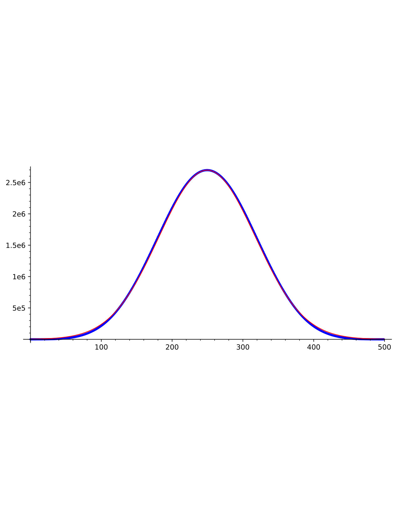 Figure 1
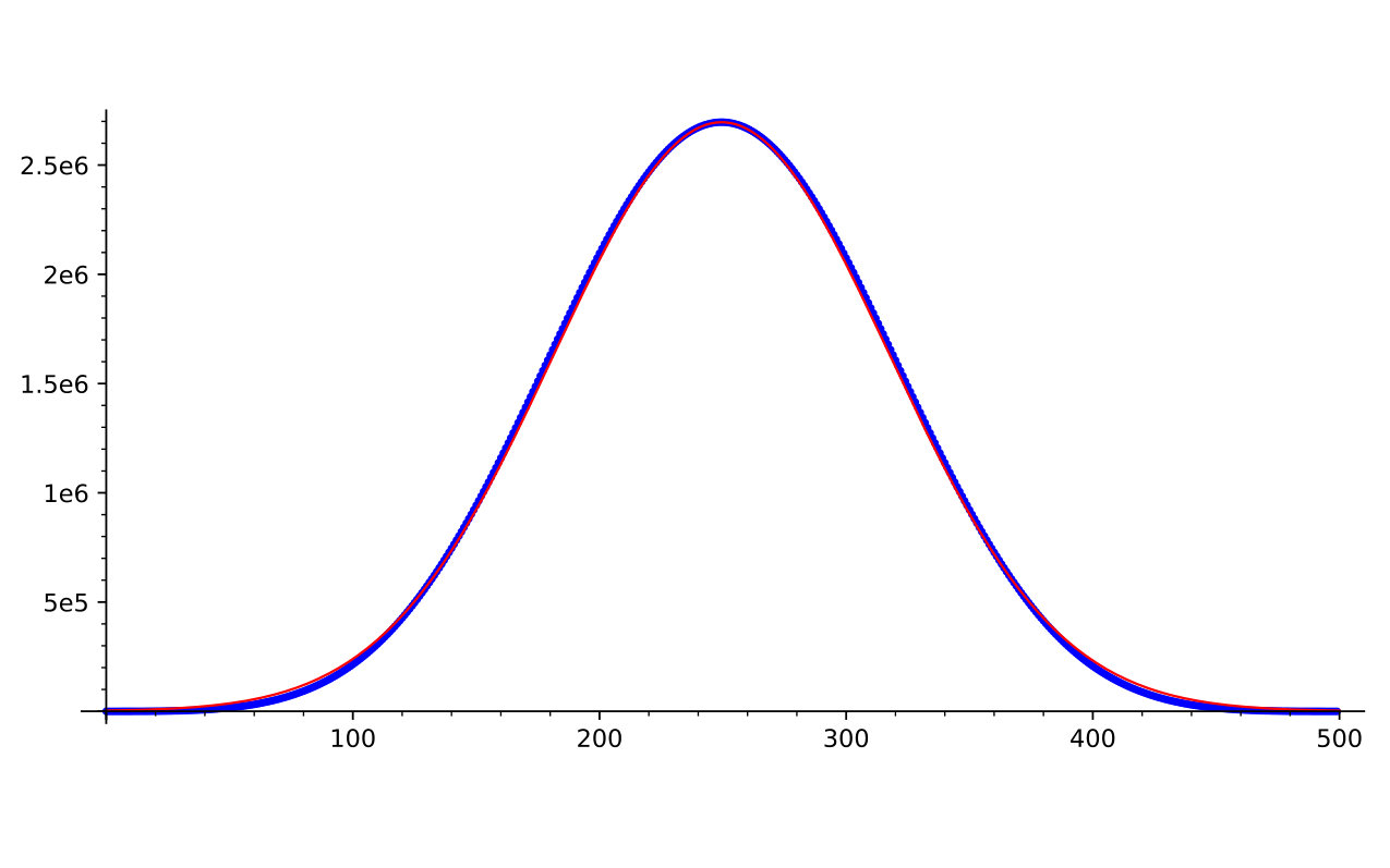 Figure 2
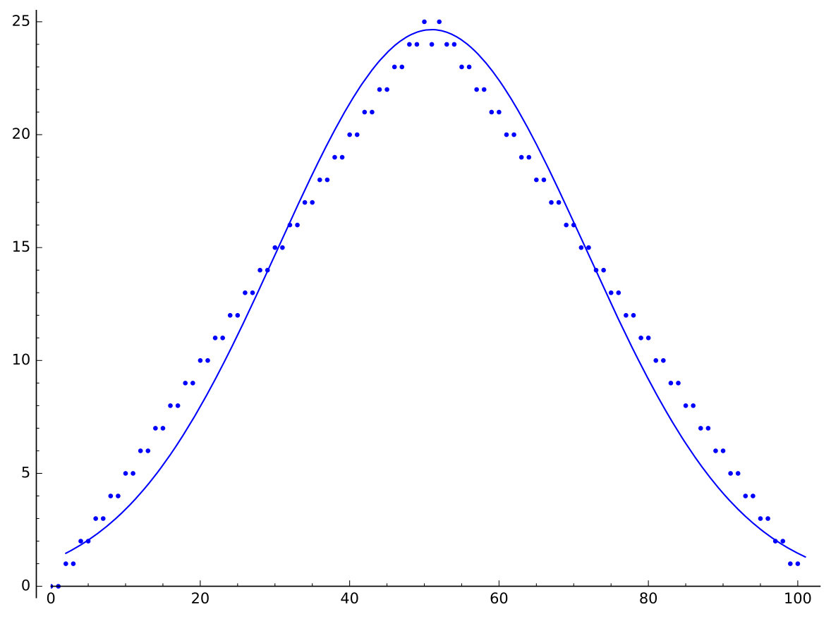 Figure 3
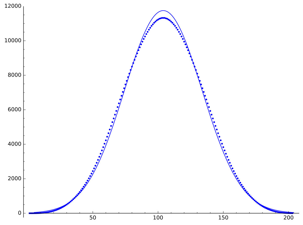 Figure 4
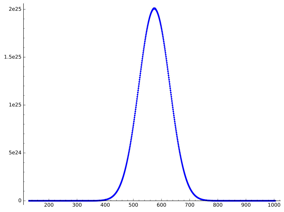 Figure 5
| Statistic | Set | Generating Function | References |
|---|---|---|---|
| elements | subsets | classical | |
| parts | strict partitions | [EL41] | |
| length/inversion number/major index | [Fel45], [Gon44] | ||
| cycles; left-to-right minima | [Fel45], [Gon44] | ||
| descents | Eulerian polynomial | [DB62, pp. 150–154] | |
| descents | conjugacy classes in | [Ful98, Thm. 1] | [Ful98, KL18] |
| blocks | set partitions | [Har67] | |
| valleys | Dyck paths | [CWW08, Cor. 3.3]; [FH85, p. 255] | |
| length/inversion number/major index | , words type | see 3.17 | |
| major index | 1.3 |
Peer Reviews
No public reviews on file for this paper yet. If you reviewed it on a platform where reviews are public (OpenReview, ICLR, NeurIPS, ICML), you can paste yours below so the community can read it here.
Videos
No videos yet. Explain this paper in a talk, walkthrough, or lecture? Add one.
Asymptotic normality of the
major index on standard tableaux
Sara C. Billey, Matjaž Konvalinka, Joshua P. Swanson
Billey: Department of Mathematics, University of Washington, Seattle, WA 98195, USA
Konvalinka: Faculty of Mathematics and Physics, University of Ljubljana, Jadranska 21, Ljubljana, Slovenia, and Institute for Mathematics, Physics and Mechanics, Jadranska 19, Ljubljana, Slovenia
Swanson: Department of Mathematics, University of California, San Diego (UCSD), La Jolla, CA 92093-0112
Abstract.
We consider the distribution of the major index on standard tableaux of arbitrary straight shape and certain skew shapes. We use cumulants to classify all possible limit laws for any sequence of such shapes in terms of a simple auxiliary statistic, , generalizing earlier results of Canfield–Janson–Zeilberger, Chen–Wang–Wang, and others. These results can be interpreted as giving a very precise description of the distribution of irreducible representations in different degrees of coinvariant algebras of certain complex reflection groups. We conclude with some conjectures concerning unimodality, log-concavity, and local limit theorems.
Key words and phrases:
major index, hook length, tableaux, asymptotic normality, Irwin–Hall distribution, cumulants
The first author was partially supported by the Washington Research Foundation and DMS-1764012 from the National Science Foundation. The second author was partially supported by Research Project BI-US/16-17-042 of the Slovenian Research Agency and research core funding No. P1-0294.
Contents
- 1 Introduction
- 2 Background on cumulants
- 3 Combinatorial background
- 4 Asymptotic normality for on
- 5 Asymptotic normality for on
- 6 Uniform sum limits for on
- 7 Discrete distributions for on
- 8 Future work
1. Introduction
The study of permutation and partition statistics is a classic topic in enumerative combinatorics. The major index statistic on permutations was introduced a century ago by Percy MacMahon in his seminal works [Mac13, Mac17]. This statistic, denoted , is defined to be the sum of the positions of the descents of the permutation in one-line notation. A descent is any position such that . At first glance, this function on permutations may be unintuitive, but it has inspired hundreds of papers and many generalizations; for example on Macdonald polynomials [HHL05], posets [ER15], quasisymmetric functions [SW10], cyclic sieving [RSW04, AS18], and bijective combinatorics [Foa68, Car75].
The following central limit theorem for on is well known and is an archetype for our results. Given a real-valued random variable , we let
[TABLE]
denote the corresponding normalized random variable with mean [math] and variance . Briefly, we say on is asymptotically normal as based on the following classical result. See Table 1 for further examples.
Theorem 1.1**.**
[Fel45*]**
Let denote the major index random variable on under the uniform distribution. Then, for all ,*
[TABLE]
where is the standard normal random variable.
In this paper, we study the distribution of the major index statistic generalized to standard Young tableaux of straight and skew shapes. The properties we discuss here naturally generalize known properties of the major index distribution on permutations. They also have representation theoretic consequences in terms of coinvariant algebras of complex reflection groups. We will briefly introduce the main results. See Section 2 for more details on the background.
Let denote the set of all standard Young tableaux of partition shape . We say is a descent in a standard tableau if comes before in the row reading word of , read from bottom to top along rows in English notation. Equivalently, is a descent in if appears in a lower row in . Let denote the major index statistic on , which is again defined to be the sum of the descents of . Figure 1 shows some sample distributions for the major index on standard tableaux for three particular partition shapes. Note that Gaussian approximations fit the data well.
In 1.1, we simply let . For partitions, the shape may “go to infinity” in many different ways. The following statistic on partitions overcomes this difficulty.
Definition 1.2**.**
Suppose is a partition. Let the aft of be
[TABLE]
Intuitively, if the first row of is at least as long as the first column, then is the number of cells not in the first row. This definition is strongly reminiscent of a representation stability result of Church and Farb [CF13, Thm. 7.1], which is proved with an analysis of the major index on standard tableaux.
Our first main result gives the analogue of 1.1 for on . In particular, it completely classifies which sequences of partition shapes give rise to asymptotically normal sequences of statistics on standard tableaux.
Theorem 1.3**.**
Suppose is a sequence of partitions, and let be the corresponding random variables for the statistic on . Then, the sequence is asymptotically normal if and only if as .
Remark 1.4**.**
In Section 5, we more generally consider on where is a block diagonal skew partition. See [BKS18, §2] for further representation-theoretic motivation and [BKS18, Thm. 6.3] for the classification of the support of on .
The generalization of 1.3 to is 5.8. Special cases of 5.8 include Canfield–Janson–Zeilberger’s main result in [CJZ11] classifying asymptotic normality for or on words (though see [CJZ12] for earlier, essentially equivalent results due to Diaconis [Dia88]). The case of words generalizes 1.1. The case of 1.3 also recovers the main result of Chen–Wang–Wang [CWW08], giving asymptotic normality for -Catalan coefficients.
Our proof of 1.3 relies on the method of moments, which requires useful descriptions of the moments of . Adin–Roichman [AR01] gave exact formulas for the mean and variance of in terms of the hook lengths of . Their argument leverages the following -analogue of the celebrated Frame–Robinson–Thrall Hook Length Formula [FRT54, Thm. 1] (obtained by setting ):
[TABLE]
where denotes the hook length of a cell in and . Equation (1) is due to Stanley [Sta99, Cor. 7.21.5] and is strongly related to the stable principal specialization of Schur functions by the identity [Sta99, Prop. 7.19.11].
In fact, formulas for the th moment , th central moment , and th cumulant of on may be derived from (1). The most elegant of these formulas is for the cumulants, from which the moments and central moments are all easy to compute.
Theorem 1.5**.**
Let and . We have
[TABLE]
where are the Bernoulli numbers.
See 2.9 for a generalization of (2) along with exact formulas for the moments and central moments. See 2.10 for the some of the history of this formula.
Remark 1.6**.**
For “most” partition shapes, one expects the term in (2) to dominate , in which case asymptotic normality is quite straightforward. However, for some shapes there is a very large amount of cancellation in (2) and determining the limit law can be quite subtle.
While can be written as the sum of scaled indicator random variables where determines if there is a descent at position , the are not at all independent, so one may not simply apply standard central limit theorems. Interestingly, the are identically distributed [Sta99, Prop. 7.19.9]. The lack of independence of the ’s likewise complicates related work by Fulman [Ful98] and Kim–Lee [KL18] considering the limiting distribution of descents in certain classes of permutations.
The non-normal continuous limit laws for on turn out to be the Irwin–Hall distributions , which are the sum of i.i.d. continuous random variables. The following result completely classifies all possible limit laws for on for any sequence of partition shapes. See 6.3 for the generalization to block diagonal skew shapes.
Theorem 1.7**.**
Let be a sequence of partitions. Then converges in distribution if and only if
- (i)
; or 2. (ii)
* and ; or* 3. (iii)
the distribution of is eventually constant.
The limit law is in case (i), in case (ii), and discrete in case (iii).
Case (iii) naturally leads to the question, when does ? Such a description in terms of hook lengths is given in 7.1. 1.7 naturally raises several open questions and conjectures concerning unimodality, log-concavity, and local limit theorems, which are described in Section 8.
Example 1.8**.**
We illustrate each possible limit in 1.7. For (i), let , so that and the distributions are asymptotically normal. For (ii), fix and let , so that is constant and the distributions converge to . For (iii), let and , which have the same multisets of hook lengths despite not being transposes of each other, and consequently the same normalized distributions.
The rest of the paper is organized as follows. In Section 2, we give background focused on cumulants aimed at the combinatorial audience. In Section 3, we collect combinatorial background on permutations, tableaux, etc, aimed more at the probabilistic audience. In Section 4, we analyze on as an introductory example. In Section 5, we classify when on is asymptotically normal. In Section 6, we determine the remaining continuous limit laws for on . In Section 7, we characterize the possible discrete distributions for on in terms of hook lengths. Finally, Section 8 lists conjectures concerning unimodality, log-concavity, and local limit theorems.
2. Background on cumulants
In this section, we review some standard terminology and results on generating functions, random variables, and asymptotic normality, with a focus on cumulants. An excellent source for many further details in this area can be found in Canfield’s Chapter 3 of [Bón15].
2.1. Exponential generating functions
We now introduce our notation for exponential generating functions and the Bernoulli numbers, which will be used with cumulants shortly.
Definition 2.1**.**
Given a rational sequence , the corresponding ordinary generating function is
[TABLE]
and the corresponding exponential generating function is
[TABLE]
Conversely, any rational power series
[TABLE]
is the ordinary generating function of the sequence and the exponential generating function of the sequence . The exponential generating functions we will encounter will all have a positive radius of convergence.
It is easy to describe products, quotients and compositions of generating functions. We recall in particular a formula for compositions of exponential generating functions for later use. Given two rational sequences , such that and , the composition of their exponential generating functions is again an exponential generating function for a rational sequence , say . For example, if and , so for all , then by [Sta99, Cor. 5.1.6], the corresponding sequence is given by and, for ,
[TABLE]
where is the collection of all set partitions of . Collecting together -orbits of in (3) quickly gives
[TABLE]
where if has parts of length , then . A more computationally efficient, recursive approach to (3) is the formula [Sta99, Prop. 5.1.7]
[TABLE]
Example 2.2**.**
The Bernoulli numbers are rational numbers determined by the exponential generating function . The first few terms in the sequence are
[TABLE]
[TABLE]
The divided Bernoulli numbers are given by for . Their exponential generating function satisfies , from which it follows that
[TABLE]
We caution that a common alternate convention for Bernoulli numbers uses with all other entries the same, corresponding with the exponential generating function .
The Bernoulli numbers have many interesting properties; see [Maz08, Wik17] and [GKP89, Section 6.5]. For example, they appear in the polynomial expansion of the sums of th powers,
[TABLE]
Compare the formula for sums of th powers to the Riemann zeta function which can be evaluated at complex values by analytic continuation. The divided Bernoulli numbers which appear in our formula (2) satisfy .
2.2. Probabilistic generating functions
We next review basic vocabulary and notation for moments and cumulants of random variables. All random variables we encounter will have moments of all orders. See [Bil95] for more details.
Definition 2.3**.**
Let be a real-valued random variable where either is continuous with probability density function or is discrete with probability mass function . The cumulative distribution function (CDF) of is given by
[TABLE]
depending on whether is continuous or discrete. For any continuous real-valued function , there is an associated random variable . The expectation of is given by
[TABLE]
The mean and variance of are, respectively,
[TABLE]
For , the th moment and th central moment of are, respectively,
[TABLE]
The moment-generating function of is
[TABLE]
which for us will always have a positive radius of convergence. The characteristic function of is
[TABLE]
which exists for all and which is the Fourier transform of , the density or mass function associated to .
Example 2.4**.**
Let be a finite set with an integer statistic . We will use the notation
[TABLE]
for the corresponding polynomial generating function. If , define a random variable associated with sampled uniformly on by The probability generating function for is
[TABLE]
Letting , an easy computation shows that the moment-generating function and characteristic function of are
[TABLE]
These expressions reveal an intimate connection between the study of generating functions of combinatorial statistics evaluated on the unit circle and the underlying probability distribution via the Laplace and Fourier transforms. In particular, the distribution determines the characteristic function and the moment-generating function, and conversely each of these determines the distribution.
Definition 2.5**.**
The cumulants of are defined to be the coefficients of the exponential generating function
[TABLE]
While cumulants of random variables may initially be less intuitive than moments, they lead to nicer formulas in many cases, including 1.5, and they often have more useful properties. See [NS11] for some history and applications. We will use the following properties of cumulants. The proofs are straightforward from the definitions.
(Familiar Values) The first three cumulants are , , and . The higher cumulants typically differ from the moments and central moments. 2. 2.
(Shift Invariance) The second and higher cumulants of agree with those for for . 3. 3.
(Homogeneity) The th cumulant of is for . 4. 4.
(Additivity) The cumulants of the sum of independent random variables are the sums of the cumulants. 5. 5.
(Polynomial Equivalence) The cumulants, moments, and central moments are determined by polynomials in any one of these three sequences.
The polynomial equivalence property can be made explicit by the results in Section 2.1. Equation (5) allows us to express the th moment of as a polynomial function of the first cumulants of and vice versa via the recurrence
[TABLE]
Using the shift invariance property of cumulants, the corresponding formula for the central moments in terms of the cumulants can be obtained from (7) by setting and leaving the other cumulants alone. This gives, for ,
[TABLE]
For instance, at we have
[TABLE]
Setting yields as mentioned above.
2.3. Cumulant formulas
Next we describe the cumulants of some well-known distributions and use one of them to deduce a result of Hwang–Zacharovas, which immediately yields 1.5 as a corollary.
Example 2.6**.**
Let be the normal random variable with mean and variance . The density function of is . Taking the Fourier transform gives the characteristic function , so the moment-generating function is and the cumulants are
[TABLE]
Using (4) to compute the central moments of from (9), we effectively set and note that only contributes, in which case . It follows that
[TABLE]
Example 2.7**.**
Let be the continuous uniform random variable whose density takes the value on the interval and [math] otherwise. Then the moment generating function is , so the cumulant generating function coincides with the exponential generating function for the divided Bernoulli numbers from Section 2.1. That is, for .
Recall from Section 1, is the Irwin–Hall distribution obtained by adding independent, identically distributed random variables. By Additivity, the th cumulant of is . More generally, let be the sum of independent uniform continuous random variables. Then the th cumulant of for is
[TABLE]
by the Homogeneity and Additivity Properties of cumulants.
Example 2.8**.**
Let be the discrete uniform random variable supported on . The probability generating function for is , so the cumulant generating function is
[TABLE]
It follows that for , the divided Bernoulli numbers arise again in this context,
[TABLE]
Product formulas for polynomials such as Stanley’s formula (1) give rise to explicit formulas for cumulants and moments according to the following theorem. The proof is immediate from 2.8 and the exponential generating function identity (4).
Theorem 2.9**.**
Suppose and are multisets of positive integers such that
[TABLE]
so in particular each . Let be a discrete random variable with . Then the th cumulant of is
[TABLE]
where is the th Bernoulli number (with ). Moreover, the th central moment of is
[TABLE]
and the th moment of is
[TABLE]
Remark 2.10**.**
Equation (12) appeared explicitly in the work of Hwang–Zacharovas [HZ15, §4.1] building on the work of Chen–Wang–Wang [CWW08, Thm. 3.1], who in turn used an argument going back at least to Sachkov [Sac97, §1.3.1]. It was rediscovered experimentally through (14) by the present authors, and by Thiel–Williams [TW18].
One frequently encounters polynomials of the form for some , as in (1). The formulas in 2.9 remain valid in this case except that one must add to the expression for and add to each factor in the product in (14) for which .
Remark 2.11**.**
The generating function machinery used to construct the cumulants in (12) works whether or not the function is polynomial. The corresponding ’s are called formal cumulants in the literature.
2.4. Asymptotic normality
Asymptotic normality is a very old topic lying at the intersection of probability and combinatorics. For an introduction, we recommend Canfield’s Chapter 3 in [Bón15].
Definition 2.12**.**
Let and be real-valued random variables with cumulative distribution functions and , respectively. We say converges in distribution to , written , if for all at which is continuous we have
[TABLE]
Recall from the introduction that for a real-valued random variable with mean and variance , the corresponding normalized random variable is
[TABLE]
Observe that has mean and variance . The moments and central moments of agree for and are given by
[TABLE]
Similarly, the cumulants of are given by , , and for .
Definition 2.13**.**
Let be a sequence of real-valued random variables. We say the sequence is asymptotically normal if .
The “original” asymptotic normality result is as follows. Let be the set of all subsets of . Let denote the random variable given by the cardinality, where is given the uniform distribution. This has the same distribution as the number of heads after fair coin flips, so the probability generating function up to normalization is . The following result is credited to de Moivre and Laplace; see [Bón15, Theorem 3.2.1] for further discussion.
Theorem 2.14** (de Moivre–Laplace).**
The sequence is asymptotically normal.
Asymptotic normality results for combinatorial statistics are plentiful. See Table 1 for more examples and further references.
2.5. The method of moments
We next describe two standard criteria for establishing asymptotic normality or more generally convergence in distribution of a sequence of random variables.
Theorem 2.15** (Lévy’s Continuity Theorem, [Bil95, Theorem 26.3]).**
A sequence of real-valued random variables converges in distribution to a real-valued random variable if and only if, for all ,
[TABLE]
Theorem 2.16** **(Frechét–Shohat Theorem,
[Bil95, Theorem 30.2]).
Let be a sequence of real-valued random variables, and let be a real-valued random variable. Suppose the moments of and all exist and the moment generating functions all have a positive radius of convergence. If
[TABLE]
then converges in distribution to .
By 2.15, we may test for asymptotic normality by checking if the normalized characteristic functions tend point-wise to the characteristic function of the standard normal. Likewise by 2.16 we may instead perform the check on the level of individual normalized moments, which is often referred to as the method of moments. By (7) we may further replace the moment condition (15) with the cumulant condition
[TABLE]
For instance, we have the following explicit criterion.
Corollary 2.17**.**
A sequence of real-valued random variables on finite sets is asymptotically normal if for all we have
[TABLE]
In fact, one may show a converse of the Frechét–Shohat theorem holds for quotients as in 2.9, though we will not have need of it here.
2.6. Local limit theorems
Asymptotic normality concerns cumulative distribution functions, so it gives estimates for the number of combinatorial objects with a large range of statistics. However, our original motivation was to count combinatorial objects with a given statistic. Estimates of this latter form are frequently referred to as local limit theorems. Here we review two motivating examples.
The present work was partly inspired by the following local limit theorem due to the third author with a uniform rather than normal limit law. For , let be modulo .
Theorem 2.18**.**
[Swa18, Theorem 1.9]** For , let denote the random variable on . Suppose . Then, for all ,
[TABLE]
Further motivation was provided by the following analogue of 3.16.
Theorem 2.19**.**
[CJZ11, Theorem 4.5]** There exists a positive constant such that for every , the following is true. Uniformly for all compositions such that and all integers ,
[TABLE]
where denotes inversions on words of type .
3. Combinatorial background
3.1. Combinatorial background for on
Here we introduce the two most well-known permutation statistics, and , as well as one unusual permutation statistic, .
Definition 3.1**.**
Let be a permutation of . Set
[TABLE]
Following Zabrocki [Zab03] for the nomenclature, we also set
[TABLE]
The equidistribution of and on is due to MacMahon, who also first introduced . His proof gave the following generating function expression for both statistics.
Theorem 3.2** ([Mac13, Art. 6]).**
We have
[TABLE]
The statistic appeared in the context of extended affine Weyl groups and Hecke algebras in the work of Iwahori and Matsumoto in 1965 [IM65]. It is the Coxeter length function restricted to coset representatives of the extended affine Weyl group of type mod translations by coroots. Stembridge and Waugh [SW98, Remarks 1.5 and 2.3] give a careful overview of this topic and further results. In particular, they prove the following factorization formula for the generating function associated to on . From this factorization, the corresponding cumulants can be read off from 2.9.
Theorem 3.3**.**
[TABLE]
Corollary 3.4**.**
The th cumulant for on is
[TABLE]
Remark 3.5**.**
Indeed, (18) holds with replaced by for any fixed if the factor of is deleted from the right-hand side. See [Zab03] for a bijective proof of this generalization. In addition, [SW98, Thm. 1.1] gives another generalization of the product formula (18) to all crystallographic Coxeter groups.
3.2. Combinatorial background for on
and
Here we review standard combinatorial notions related to words, tableaux, and their major index generating functions.
Definition 3.6**.**
Given a word with letters , the type of is the sequence where is the number of times appears in . Such a sequence is a (weak) composition of , written as . Trailing [math]’s are often omitted when writing weak compositions, so for some . Note that a word of type is a permutation in the symmetric group written in one-line notation. Just as for permutations, the inversion number of is
[TABLE]
The descent set of is
[TABLE]
and the major index of is
[TABLE]
Definition 3.7**.**
Let . We use the following standard -analogues:
[TABLE]
Example 3.8**.**
The identity statistic on the set has generating function . The “sum” statistic on has generating function .
For , let denote the words of type . MacMahon’s classic result generalizing 3.2 in fact shows that and have the same distribution on .
Theorem 3.9** ([Mac13, Art. 6]).**
For each ,
[TABLE]
Definition 3.10**.**
A composition such that is called a partition of , written as . The size of is and the length of is the number of non-zero entries. The Young diagram of is the upper-left justified arrangement of unit squares called cells where the th row from the top has cells following the English notation; see Figure 2(a). The hook length of a cell is the number of cells in in the same row as to the right of and in the same column as and below , including itself; see Figure 2(b). A corner of is any cell with hook length . A bijective filling of is any labeling of the cells of by the numbers .
Definition 3.11**.**
A skew partition is a pair of partitions such that the Young diagram of is contained in the Young diagram of . The cells of are the cells in the diagram of which are not in the diagram of , written . We identify straight partitions with skew partitions where is the empty partition. The size of is . The notions of bijective filling, hook lengths, and corners naturally extend to skew partitions as well.
Definition 3.12**.**
Given a sequence of partitions , we identify the sequence with the block diagonal skew partition obtained by translating the Young diagrams of the so that the rows and columns occupied by these components are disjoint, form a valid skew shape, and appear in order from top to bottom as depicted in Figure 3.
Definition 3.13**.**
A standard Young tableau of shape is a bijective filling of the cells of such that labels increase to the right in rows and down columns; see Figure 4. The set of standard Young tableaux of shape is denoted . The descent set of is the set of all labels in such that is in a strictly lower row than . The major index of is
[TABLE]
Remark 3.14**.**
The block diagonal skew partitions allow us to simultaneously consider words and tableaux as follows. Recall that is set of all words with type . Letting , we have a bijection
[TABLE]
which sends a tableau to the word whose th letter is the row number in which appears in , counting from the bottom up rather than top down. For example, using the skew tableau on the right of Figure 4, we have . It is easy to see that , so that . Hence .
Remark 3.15**.**
We also recover -integers, -binomials, -multinomials, and -Catalan numbers up to -shifts as special cases of the major index generating function for tableaux given in (1):
[TABLE]
Many combinatorial statistics arise from sets indexed by more complicated objects than the positive integers, in which case one can “let ” in many different ways. The following result due to Canfield, Janson, and Zeilberger illustrates a more interesting limit. Their result is characterized by the statistic where with .
Theorem 3.16**.**
[CJZ11, Theorem 1.2]** Let be a sequence of compositions, possibly of differing lengths. Let be the inversion (or major index) statistic on words of type . Then is asymptotically normal if and only if
[TABLE]
Remark 3.17**.**
Explorations equivalent to 3.16 appeared significantly earlier than [CJZ11] in other contexts, for instance [Dia88, p. 127-128] and (in the two-letter case) [MW47]. See [CJZ12] for further discussion and references.
The cumulant formula for , 1.5, follows immediately from 2.9 and Stanley’s formula (1). Adin and Roichman [AR01] had previously used (1) to compute the mean and variance of as
[TABLE]
and
[TABLE]
The following common generalization of Stanley’s formula (1) and MacMahon’s formula, 3.9, is well known (e.g. see [Ste89, (5.6)]). See [BKS18, Thm. 2.15] for other applications.
Theorem 3.18**.**
Let where and . Then
[TABLE]
Corollary 3.19**.**
Let be the th cumulant of on for . Then
[TABLE]
For general skew shapes, does not factor as a product of cyclotomic polynomials times to a power. A “-Naruse” formula due to Morales–Pak–Panova, [MPP18, (3.4)], gives an analogue of (1) involving a sum over “excited diagrams,” though the resulting sum has a single term precisely for the block diagonal skew partitions .
4. Asymptotic normality for on
We give with a straightforward example which serves as a warmup and establishes some notation. See Section 3.1 for background. Asymptotic normality of on follows from the cumulant formula in 3.4 by the following routine calculations. Recall that means that .
Lemma 4.1**.**
Fix . Then, as ,
[TABLE]
Proof.
We have
[TABLE]
∎
Remark 4.2**.**
The value of the integral in 4.1 is well known:
[TABLE]
See [OEI17, A002457] for a surprisingly large number of interpretations of the reciprocals of these values. Equation (23) is also a very special case of the Selberg integral formula [Sel44], which has many interesting connections to algebraic combinatorics such as those in [KO17].
Corollary 4.3**.**
Fix . Let be the th cumulant of on , and let be the th cumulant of the corresponding normalized random variable with mean [math] and variance . Then, uniformly for all , we have
[TABLE]
That is, there are constants depending only on such that
[TABLE]
Proof.
It follows immediately from 3.4 and 4.1 that . Hence
[TABLE]
∎
Theorem 4.4**.**
Let be the random variable for the statistic taken uniformly at random from . Then, is asymptotically normal.
Proof.
For fixed even, we have , so by 4.3, as . The odd cumulants for vanish since the odd Bernoulli numbers are [math]. The result now follows from 2.17. ∎
Remark 4.5**.**
A key step in the above argument was to show that the variance of on satisfies . Indeed, the argument gives . The weaker observation that is the dominant contribution to is essentially enough to deduce asymptotic normality in this case. Our analysis of on standard tableaux includes non-normal limits, so more precise estimates like the above will become absolutely necessary. A straightforward modification of the above argument together with 3.2 also proves 1.1.
5. Asymptotic normality for on
The main result of this section, 5.8, classifies the sequences of block diagonal skew partitions for which is asymptotically normal. We begin with a series of estimates for the differences , culminating in 5.7.
Definition 5.1**.**
A reverse standard Young tableau of shape is a bijective filling of which strictly decreases along rows and columns. The set of reverse standard Young tableaux of shape is denoted .
Lemma 5.2**.**
Let and . Then for all ,
[TABLE]
Furthermore, for any positive integer ,
[TABLE]
where denotes the complete homogeneous symmetric function.
Proof.
For (25), equality holds at the outer corner where . Removing and subtracting from each remaining entry in allows us to induct. Equation (26) follows immediately by rearranging the terms and factoring . ∎
Lemma 5.3**.**
Let such that . Let be any positive integer. Then
[TABLE]
Proof.
Using Riemmann sums for , we obtain the bounds
[TABLE]
for all positive integers . The upper bound in the lemma now follows immediately.
For the lower bound, label the cells of by some . By (25), , and by assumption we have for all . Considering the tighter of these two bounds on each summand and using (27) again, we have
[TABLE]
Consequently,
[TABLE]
It is easy to check that the coefficient on is bounded below by for all positive integers . The result follows. ∎
Definition 5.4**.**
Given any partition , let the aft of be the statistic
[TABLE]
where is the number of cells in the same row as to the right of , including itself, and is the number of cells in the same column as below , including . When , we have as above. When , we have . Note that .
Lemma 5.5**.**
Let such that , and let be any positive integer. Furthermore, suppose . Then,
[TABLE]
Proof.
The result holds trivially if since in that case is a single row or column, so assume . Let have , where we may assume is the first cell in its row and column. For convenience, we may further assume by symmetry that . Since , it also follows that .
Now let be the set of cells in the row of , not including itself, which are the only cells of in their columns. Since is a skew partition, is connected. We claim that . To prove the claim, we first observe that the hypothesis implies there are at most cells of which could possibly be in the columns of the cells of the row of not including . Since and , we have . Hence no more than of the cells in the row of not including can be excluded from , so for .
Construct iteratively as follows; see Figure 5 for an example. At each step of the iteration, we will first increment all existing labels by and then label a new outer cell with . Begin by adding the cells of the row of from left to right until the last cell of has been added. Now add the remaining cells of row by row starting at the topmost row and going from left to right. It is easy to see that the result respects the decreasing row and column conditions, so .
By 5.2, we have inequalities . At every step of the iteration, a labeled cell has increase by , while increases by if and only if the newly labeled cell is in the hook of . That is, for the final filling , counts the number of times after cell was filled that the new cell was not in the same row or column as . For each , it follows that .
For the lower bound, we now find
[TABLE]
where the first inequality uses the fact that has pointwise lower bounds of and the last inequality uses (27).
For the upper bound, we construct a new as follows; see Figure 6 for an example. First, for each cell in the row of taken from left to right, add the topmost cell in the column of . Now add the remaining cells of exactly as before. Again consider the final differences . For cells added in the second stage, could increase no more than times, so for such . For cells added in the first stage, we claim that . For the claim, it suffices to show that after the first stage, for cells added in the first stage, . During the first stage, the differences are zero while cells of row are being added. Afterwards during the first phase, cells not in row are added, of which there are no more than , so the differences can increase no more than many times during the first phase, completing the claim.
Having established that , we now find by (26) and (27),
[TABLE]
∎
Corollary 5.6**.**
For fixed , uniformly for all skew shapes ,
[TABLE]
Proof.
Let . When , the result follows from 5.5. On the other hand, when , then , and the result follows from 5.3. ∎
Corollary 5.7**.**
Fix to be an even positive integer. Uniformly for all block diagonal skew shapes , the absolute value of the normalized cumulant of is .
Proof.
For even, by (22) and 5.6, we have
[TABLE]
where . Consequently by the homogeneity of cumulants, we have
[TABLE]
∎
We now state and prove the generalization of 1.3 for the block diagonal skew shapes from Section 3.2.
Theorem 5.8**.**
Suppose is a sequence of block diagonal skew partitions, and let be the corresponding random variables for the statistic. Then, the sequence is asymptotically normal if and only if as .
Proof.
If , the result follows immediately from 2.17, 5.7, and the fact that the odd cumulants vanish. On the other hand, if , in the next section we will show that has a subsequence which converges to either a discrete or uniform-sum distribution, which in either case is non-normal. ∎
Remark 5.9**.**
Using work of Hwang–Zacharovas [HZ15, Thm. 1.1], considering just the case is sufficient to prove both directions of 5.8. However, the estimates we’ve given for are strong enough to bound all the normalized cumulants simultaneously, and restricting to (or even ) does not simplify the argument.
6. Uniform sum limits for on
The estimates from Section 5 apply when . We next give an analogous estimate handling the case when is bounded, resulting in 6.2. We may then deduce 1.7 from the introduction and its generalization to block diagonal skew shapes, 6.3. Recall from Section 1 and 2.7 that is the Irwin–Hall distribution obtained by adding i.i.d. random variables.
Lemma 6.1**.**
Suppose is a sequence of skew partitions such that and
[TABLE]
Then for each fixed , we have
[TABLE]
Proof.
Take large enough so that and . Let be such that so is the first cell in its row and column, as in the proof of 5.5. Consider three regions of :
- (i)
The rightmost cells in the row of . 2. (ii)
The remaining leftmost cells in the row of . 3. (iii)
The remaining cells in .
Construct iteratively as in the proof of 5.5 as follows. First add cells in region (iii) row by row starting at the topmost row proceeding from left to right, stopping just before inserting the row of . Next add the cells from region (ii) from left to right. Now add the remaining cells in region (iii) row by row starting at the row immediately below the row of proceeding from left to right. Finally insert the cells from region (i) from left to right. It is easy to see that the cells in region (i) are the lowest cells in their column, from which it follows that indeed satisfies the column and row decreasing conditions.
We now consider the contributions of regions (i)-(iii) to the quotient
[TABLE]
Recall that can be interpreted as the number of times a cell inserted after cell was not inserted in the same hook as . It follows that for region (i), leaving only contributions from the cells in regions (ii) and (iii), a bounded sum. For region (ii), we have , so that
[TABLE]
Dividing by , cells in region (ii) contribute [math] to the sum in the limit. Finally, for region (iii), we find and , so that for each of the cells in region (iii),
[TABLE]
Dividing by , both bounds are asymptotic to as . Adding up all such contributions, the result follows. ∎
Theorem 6.2**.**
Suppose that is a sequence of block diagonal skew partitions such that and is constant. Let be the corresponding random variable for the statistic. Then converges in distribution to .
Proof.
Using Equation 22 and 6.1, we have for that
[TABLE]
From 2.7 and the homogeneity and additivity properties of cumulants, we have
[TABLE]
The result now follows from 2.16 after converting moments to cumulants. ∎
Theorem 6.3**.**
Let be a sequence of block diagonal skew partitions. Then the sequence converges in distribution if and only if
- (i)
; or 2. (ii)
* and ; or* 3. (iii)
the distribution of is eventually constant.
The limit law is in case (i), in case (ii), and discrete in case (iii).
Proof.
The backwards direction follows from 5.8 and 6.2. In the forwards direction, let be such a sequence where converges in distribution. If is bounded, then there are only finitely many distinct , forcing case (iii). If is unbounded, then we have subsequences satisfying either (i) or (ii) since the sequence converges in distribution, which from 5.8 and 6.2 gives convergence in distribution to or , which are continuous, distinct distributions. The result follows. ∎
From the Central Limit Theorem, we know the Irwin–Hall distribution for large closely resembles a normal distribution, so it will be quite rare for a plot of the coefficients of to look anything but normal. Since Irwin–Hall distributions are finitely supported, the difference between the two distributions is mainly in the tails. We note that even for , there is a close resemblance. See the plot in Figure 7.
7. Discrete distributions for on
We conclude by analyzing more carefully the discrete case of the limit law classification for on , 1.7. The result is 7.1, which lists several families of pairs of shapes and of differing sizes for which we nonetheless have .
A well-known corollary of (1) is that for partitions and of , is equidistributed on and if and only if and the multisets and are equal. These hook multisets do not entirely characterize the partition—see [HC78]. The following theorem gives a similar result even if we consider the corresponding standardized random variables and .
Theorem 7.1**.**
Let and be partitions. Then and have the same distribution if and only if
- (i)
the multisets of hook lengths and are equal; or 2. (ii)
the multisets and are equal; or 3. (iii)
* and are each either a single row or column; or* 4. (iv)
.
Moreover, case (ii) occurs if and only if, up to transposing,
- (a)
* and for ; or* 2. (b)
* and for ; or* 3. (c)
* and for ; or* 4. (d)
* and , or and .*
Proof.
Let and . Let , which is a polynomial by (1) with constant coefficient . Let . Let and be defined similarly.
In the backwards direction, if (i) holds, then , both variances agree by 1.5, and , so and have the same distribution. Similarly if (ii) holds , both variances agree, and and have the same distribution again. Condition (iii) holds if and only if the distributions are concentrated at a single point. For (iv), we have and , so the normalized distributions are clearly equal.
In the forwards direction, suppose and have the same distribution. Since has constant coefficient , is concentrated at a single point if and only if , which occurs if and only if is a single row or column which is covered by case (iii). It is easy to see that if and only if which is covered by case (iv).
Assume . By [BKS18, Thm. 1.1], it follows that and each have two adjacent non-zero coefficients. Since and each have constant term 1 and two adjacent non-zero coefficients, then it follows from the assumption and have the same distribution that
[TABLE]
Without loss of generality, we can assume . If , we have , from which it follows that the multisets of hook lengths are equal by considering multiplicities of zeros at all primitive roots of unity as in case (i).
From here on, assume . The multiplicity of a zero of a primitive th root of unity in (32) is [math] on the right, so from the left must have a hook of length so it itself is a hook shape partition. Since is not a single row or column by the assumption , we know does not have a cell with hook length . Consequently, the multiplicity of a zero at a primitive th root of unity in (32) is on the left, forcing on the right. Thus (32) becomes
[TABLE]
and as before the multiset condition (ii) must hold. This completes the proof of the first statement in the theorem.
For the second statement, suppose (ii) holds, so the multisets and are equal. Then, and has a cell with hook length , so is a hook shape partition for some , and
[TABLE]
By transposing if necessary, we may assume is the maximum hook length in . If has one cell with hook length , then (a) holds. Otherwise, both and have precisely two cells with hook length , so is the union of two rectangles and not itself a rectangle. If were a hook, then it would have a hook length equal to which would imply has a cell of hook length contradicting the fact that has two outer corners. Thus is not itself a hook.
Transposing if necessary, we can assume its first two rows are equal, say . If , one may check that the cell furthest from the origin in the intersection of the two rectangles forming would be the only cell of its hook length, and that moreover its two neighbors in the intersection would each have one larger hook length, contrary to (34). It follows that where , , and . We now have several cases.
- •
If , the hook lengths of are . The “gap” between and together with (34) forces , so that with . Here , resulting in case (b).
- •
If , the last two columns of already contain two cells with hook length . If , the first column would also have a cell with hook length , contradicting (34), so .
- –
If , the hook lengths of are . Because of the “gap” between and , this is of the form in (34) if and only if or , resulting in case (d).
- –
Suppose . If , then the final three columns of contain three cells with hook length , contradicting (34), so . The hook lengths of are then , which is already of the form (34), resulting in case (c).
The reverse implications from (a)-(d) to (ii) were verified in the course of the above argument. ∎
Remark 7.2**.**
The proof of 7.1 applies more generally to arbitrary scaling factors and translations of the distributions of and , and not just those coming from means and variances.
8. Future work
We conjecture that almost all of the polynomials of the form are unimodal and log-concave. In this section, we discuss the deviations of each of these properties. In the rare cases where unimodality or log-concavity fails, it only seems to happen at the very beginning and end of the sequence of coefficients or near the middle coefficient.
Recall that a polynomial is unimodal if
[TABLE]
for some , and is log-concave if for all integers . A polynomial with nonnegative coefficients which is log-concave and has no internal zero coefficients is necessarily unimodal [Sta89]. By [BKS18], we know exactly where internal zeros occur so log-concavity would imply unimodality in these cases.
We say is nearly unimodal if instead
[TABLE]
for some and has symmetric coefficients. Also, a symmetric polynomial is nearly log-concave if for all .
Conjecture 8.1**.**
The polynomial is unimodal if has at least corners. If has corners or fewer, then is unimodal except when or is among the following partitions:
- (1)
Any partition of rectangle shape that has more than one row and column. 2. (2)
Any partition of the form with and even. 3. (3)
Any partition of the form with and even. 4. (4)
Any partition of the form with and even. 5. (5)
Any partition of the form with . 6. (6)
Any partition on the list of 40 special exceptions:
[TABLE]
8.1 was checked for all partitions up to size . Each of the families , , or have a relatively simple set of hook lengths so explicit formulas can be derived for the coefficients of . We have found explicit proofs of near unimodality for each of these cases. They are related to known integer sequences [OEI17, A266755] and [OEI17, A008642] with nice generating functions. Furthermore, these families are all nearly unimodal as well as 20 of the special exceptions. All rectangles with at least 2 rows and columns are nearly unimodal for . The only deviation occurs at up to symmetry. We conjecture this trend also continues, hence the claim that all coefficients in are close to unimodal. The family is a bit further from being unimodal. The proof of the following result is omitted, but follows directly from a careful analysis of the hook lengths.
Proposition 8.2**.**
If for any positive integer , then the maximal coefficient of , say , satisfies the equation and and is the median nonzero coefficient. Here is an indicator function which is 1 if true and 0 if false.
Conjecture 8.3**.**
The polynomials are “nearly unimodal but not unimodal” for partitions or in the following cases:
- (1)
Any partition of rectangle shape that has more than one row and column with more than 30 cells. 2. (2)
Any partition of the form with and even. 3. (3)
Any partition of the form with and even. 4. (4)
Any partition of the form with and even.
8.3 was checked for all paritions of size up to . It also holds for the following 14 special exceptions:
[TABLE]
[TABLE]
Log-concavity for the polynomials appears to be harder to characterize. There are examples of partitions with even 5 corners which are not log-concave. For example for is nearly log-concave but . The only deviation occurs at up to symmetry. Thus, we summarize what we have observed in the following conjecture.
Conjecture 8.4**.**
The polynomials are almost always log-concave for partitions for large .
This conjecture is based on the fact that the normal distribution is log-concave and the following evidence. The approximate probability that a uniformly chosen partition of has the log-concave property and the corresponding probability for the nearly log-concave property is given in the following table:
By 1.3 and the conjectured claim that the coefficients of are unimodal or almost unimodal for large , one might hope that we could approximate the number of with by the density function for the normal distribution with mean and variance . We have the following conjectured bounds on such an approximation.
Conjecture 8.5**.**
Let be any partition. Uniformly for all , for all integers , we have
[TABLE]
The conjecture has been verified for and with a constant of , which is tight up to reasonable limits on computation in the sense that if it is changed to with the other constraints the same, it fails at .
Conjecture 8.6**.**
Asymptotic normality for general skew shapes and not just block diagonal skew shapes holds if and only if as , generalizing the result in 5.8.
The argument in Section 5 proves that the “formal cumulants” associated with
[TABLE]
exhibit asymptotic normality when . However, this is only the first term in the general -Naruse formula for . One approach to 8.6 would be to show the remaining terms are “appropriately negligible.”
Acknowledgments
We would like to thank Krzysztof Burdzy, Rodney Canfield, Persi Diaconis, Sergey Fomin, Pavel Galashin, Svante Janson, William McGovern, Andrew Ohana, Greta Panova, Mihael Perman, Martin Raič, Richard Stanley, Sheila Sundaram, Vasu Tewari, Lauren Williams, and Alex Woo for helpful discussions related to this work.
The reference list from the paper itself. Each links out to its DOI / PubMed record.
- 1[AR 01] Ron M. Adin and Yuval Roichman. Descent functions and random Young tableaux. Combin. Probab. Comput. , 10(3):187–201, 2001.
- 2[AS 18] Connor Ahlbach and Joshua P. Swanson. Refined cyclic sieving on words for the major index statistic. European Journal of Combinatorics , 73:37 – 60, 2018.
- 3[Bil 95] Patrick Billingsley. Probability and measure . Wiley Series in Probability and Mathematical Statistics. John Wiley & Sons, Inc., New York, third edition, 1995. A Wiley-Interscience Publication.
- 4[BKS 18] Sara C. Billey, Matjaž Konvalinka, and Joshua P. Swanson. Tableaux posets and the fake degrees of coinvariant algebras. Preprint ar Xiv:1809.07386 , Sep 2018.
- 5[Bón 15] Miklós Bóna, editor. Handbook of enumerative combinatorics . Discrete Mathematics and its Applications (Boca Raton). CRC Press, Boca Raton, FL, 2015.
- 6[Car 75] L. Carlitz. A combinatorial property of q 𝑞 q -Eulerian numbers. Amer. Math. Monthly , 82:51–54, 1975.
- 7[CF 13] Thomas Church and Benson Farb. Representation theory and homological stability. Adv. Math. , 245:250–314, 2013.
- 8[CJZ 11] E. Rodney Canfield, Svante Janson, and Doron Zeilberger. The Mahonian probability distribution on words is asymptotically normal. Adv. in Appl. Math. , 46(1-4):109–124, 2011.