High order direct Arbitrary-Lagrangian-Eulerian schemes on moving Voronoi meshes with topology changes
Elena Gaburro, Walter Boscheri, Simone Chiocchetti, Christian, Klingenberg, Volker Springel, Michael Dumbser

TL;DR
This paper introduces a high-order accurate Arbitrary-Lagrangian-Eulerian scheme on moving Voronoi meshes that can handle topology changes, improving robustness and accuracy for hyperbolic PDEs in fluid dynamics.
Contribution
It develops a novel high-order ALE finite volume and discontinuous Galerkin scheme on dynamically regenerated Voronoi meshes with topology changes, extending existing methods.
Findings
Demonstrates high accuracy through convergence studies.
Shows robustness in vortex flows and long simulations.
Achieves substantial improvements over conforming mesh methods.
Abstract
We present a new family of very high order accurate direct Arbitrary-Lagrangian-Eulerian (ALE) Finite Volume (FV) and Discontinuous Galerkin (DG) schemes for the solution of nonlinear hyperbolic PDE systems on moving 2D Voronoi meshes that are regenerated at each time step and which explicitly allow topology changes in time. The Voronoi tessellations are obtained from a set of generator points that move with the local fluid velocity. We employ an AREPO-type approach, which rapidly rebuilds a new high quality mesh rearranging the element shapes and neighbors in order to guarantee a robust mesh evolution even for vortex flows and very long simulation times. The old and new Voronoi elements associated to the same generator are connected to construct closed space--time control volumes, whose bottom and top faces may be polygons with a different number of sides. We also incorporate…
Click any figure to enlarge with its caption.
 Figure 1
 Figure 2
 Figure 3
 Figure 4
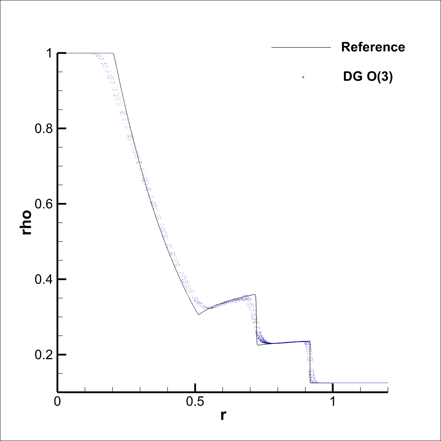 Figure 5
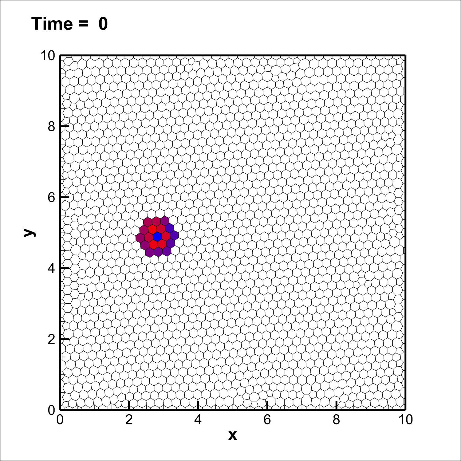 Figure 6
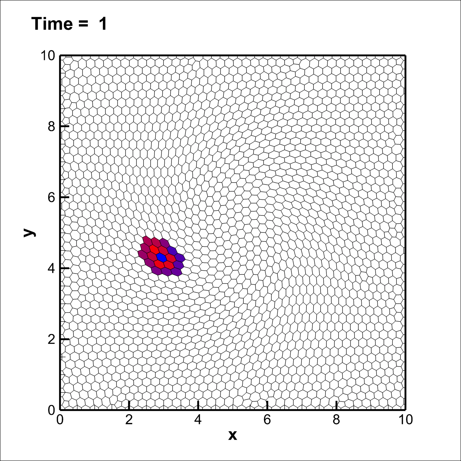 Figure 7
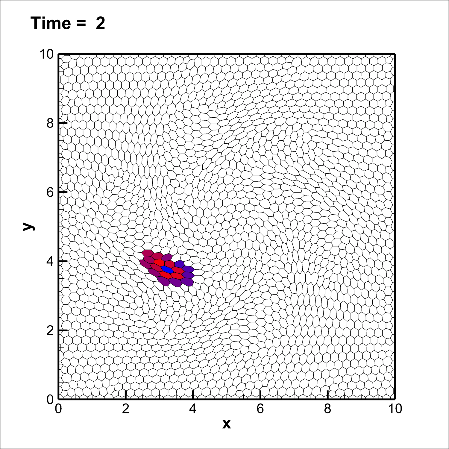 Figure 8
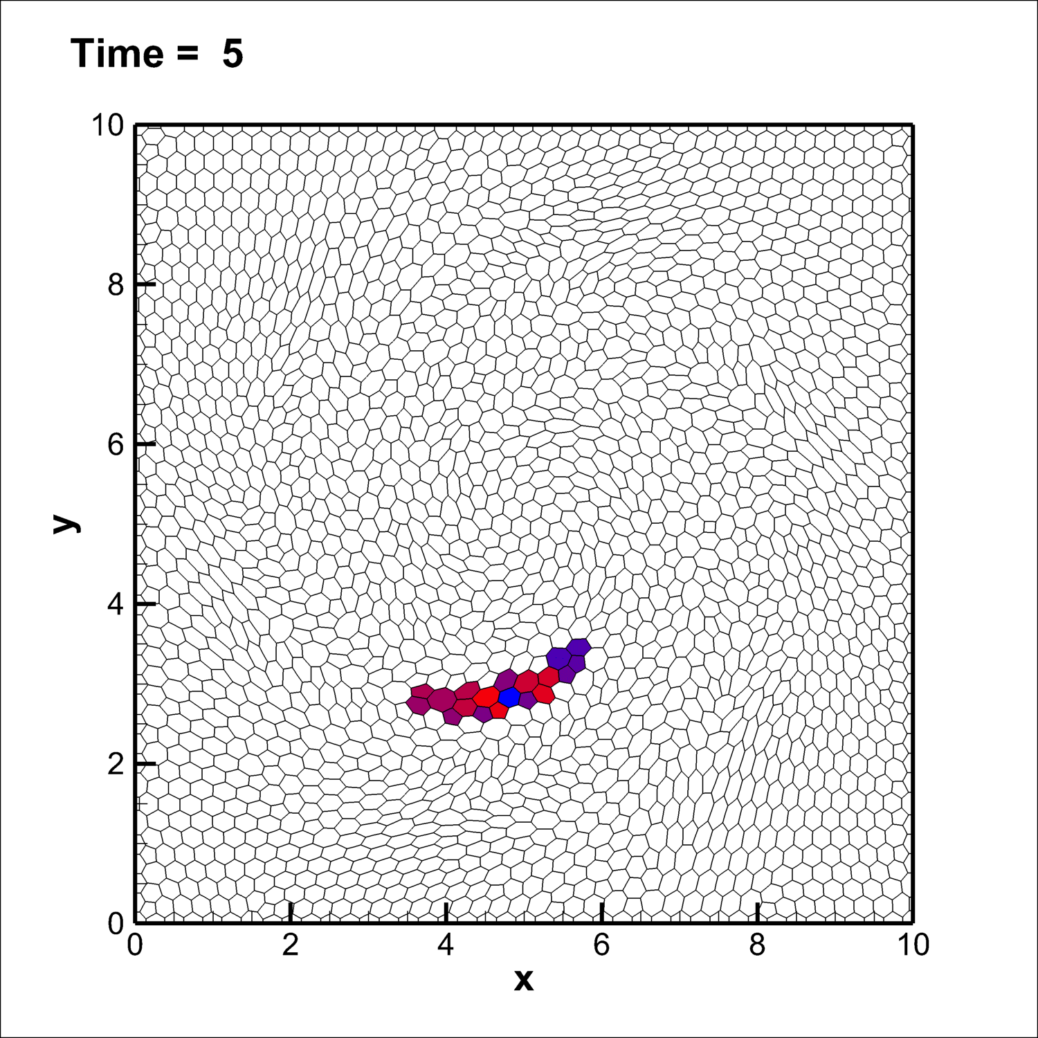 Figure 9
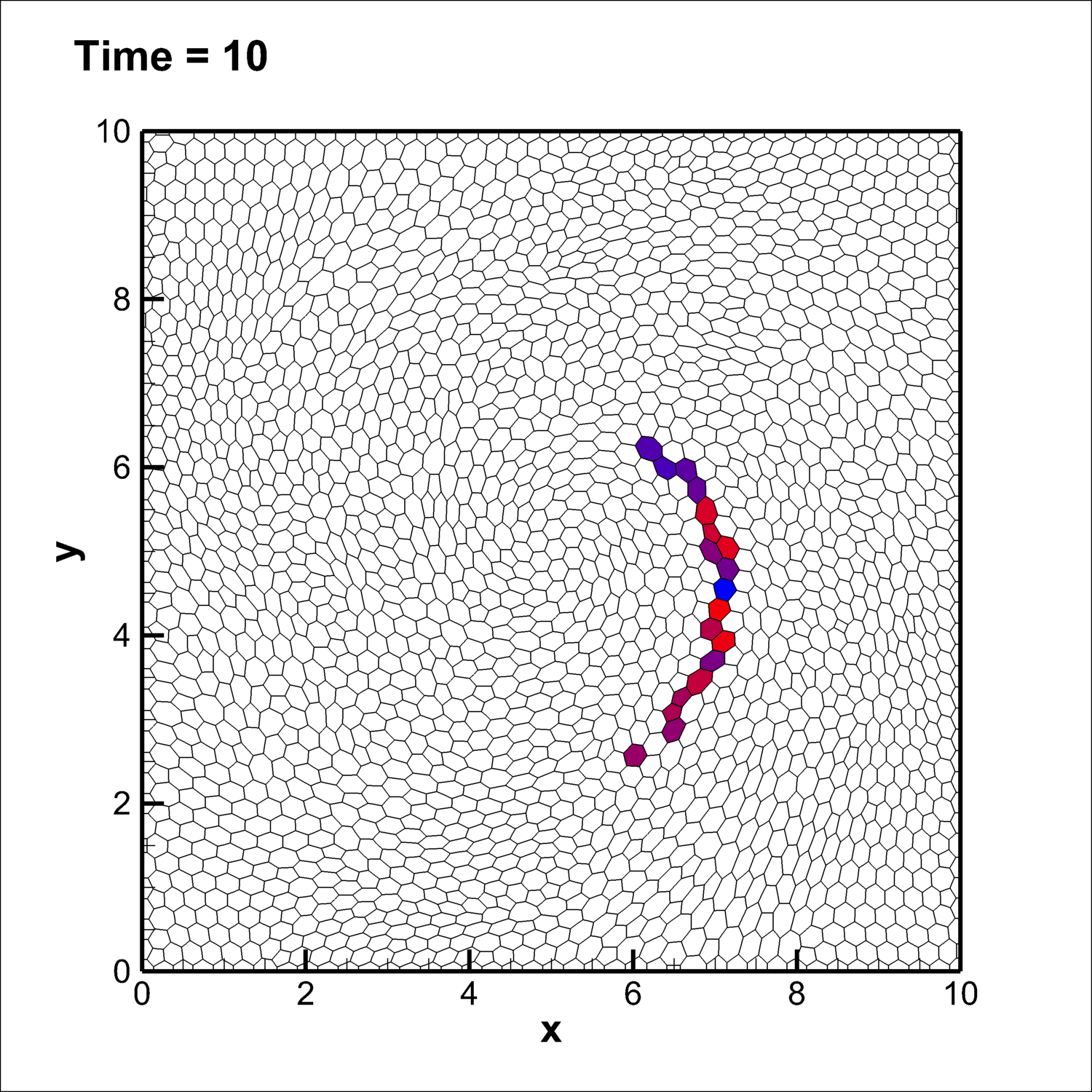 Figure 10
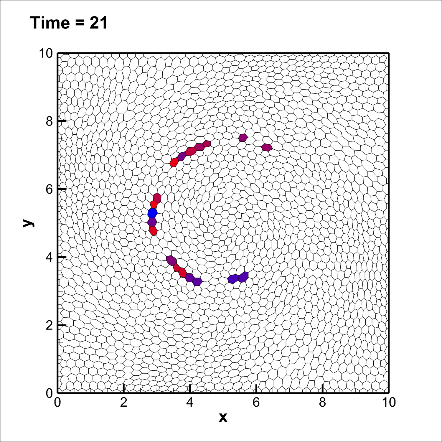 Figure 11
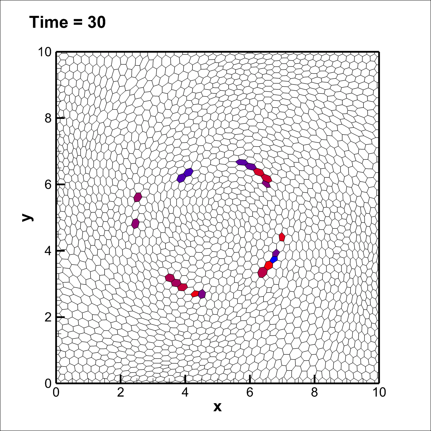 Figure 12
 Figure 13
 Figure 14
 Figure 15
 Figure 16
 Figure 17
 Figure 18
 Figure 19
 Figure 20
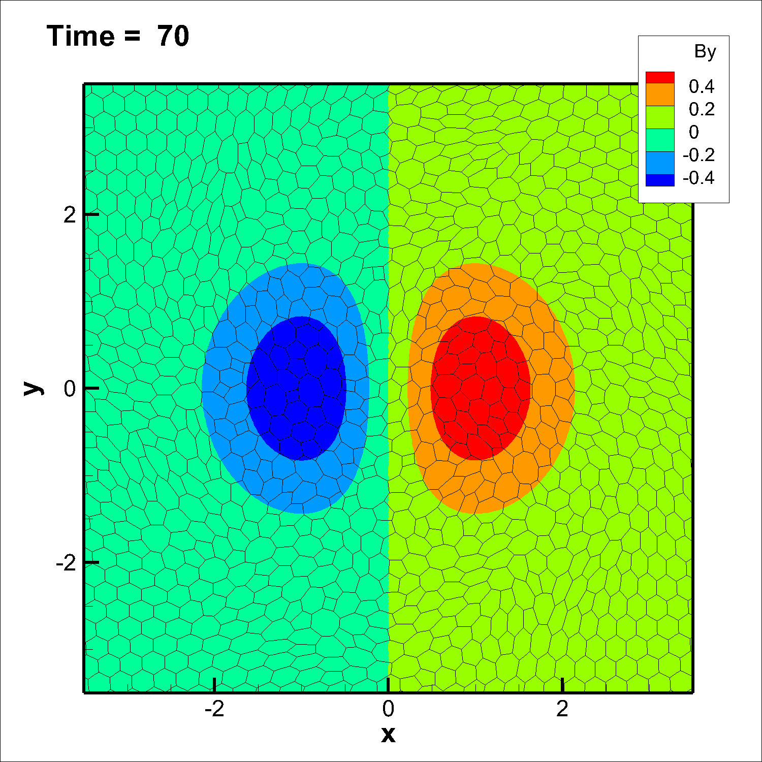 Figure 21
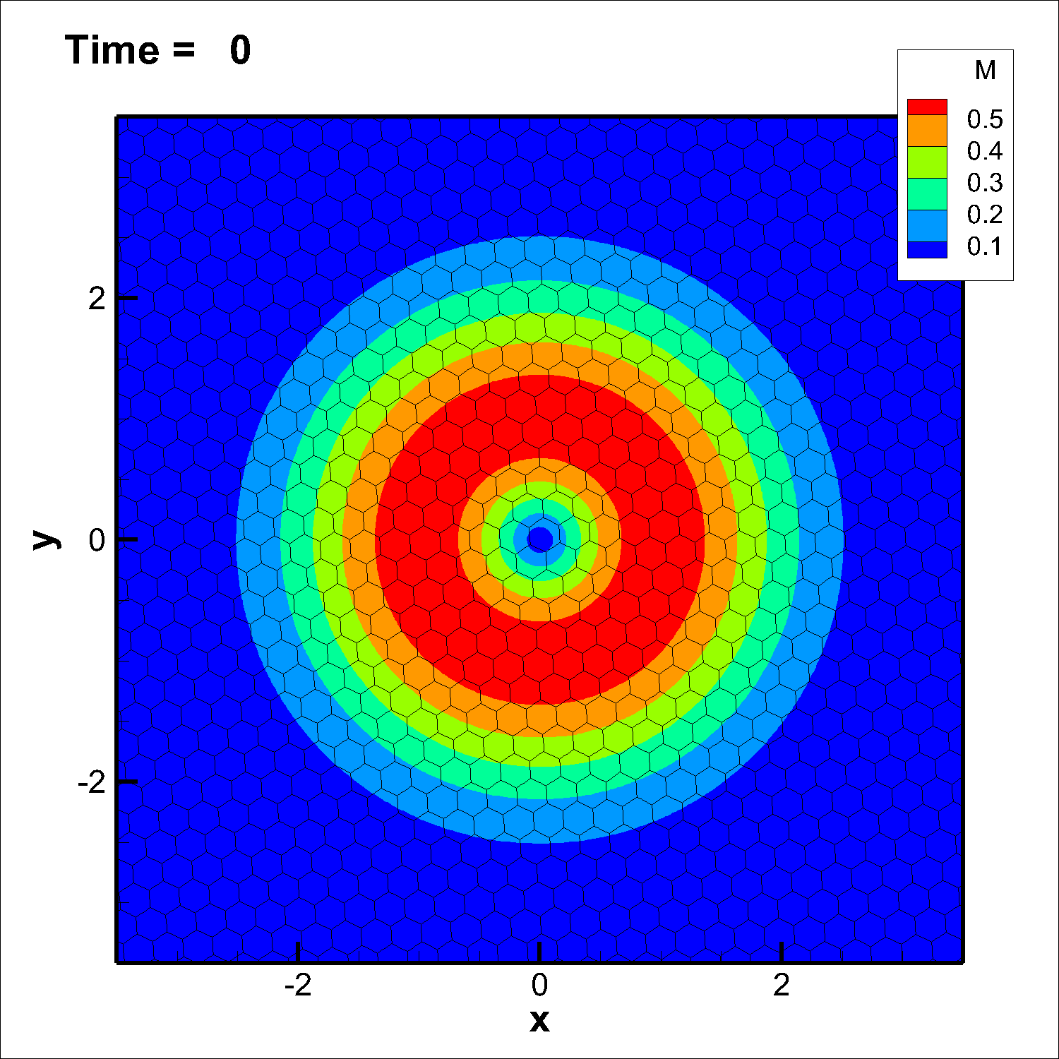 Figure 22
 Figure 23
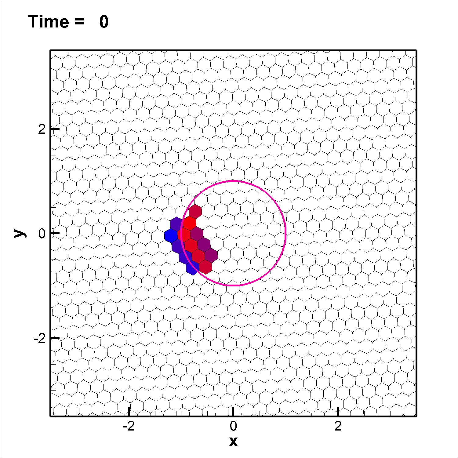 Figure 24
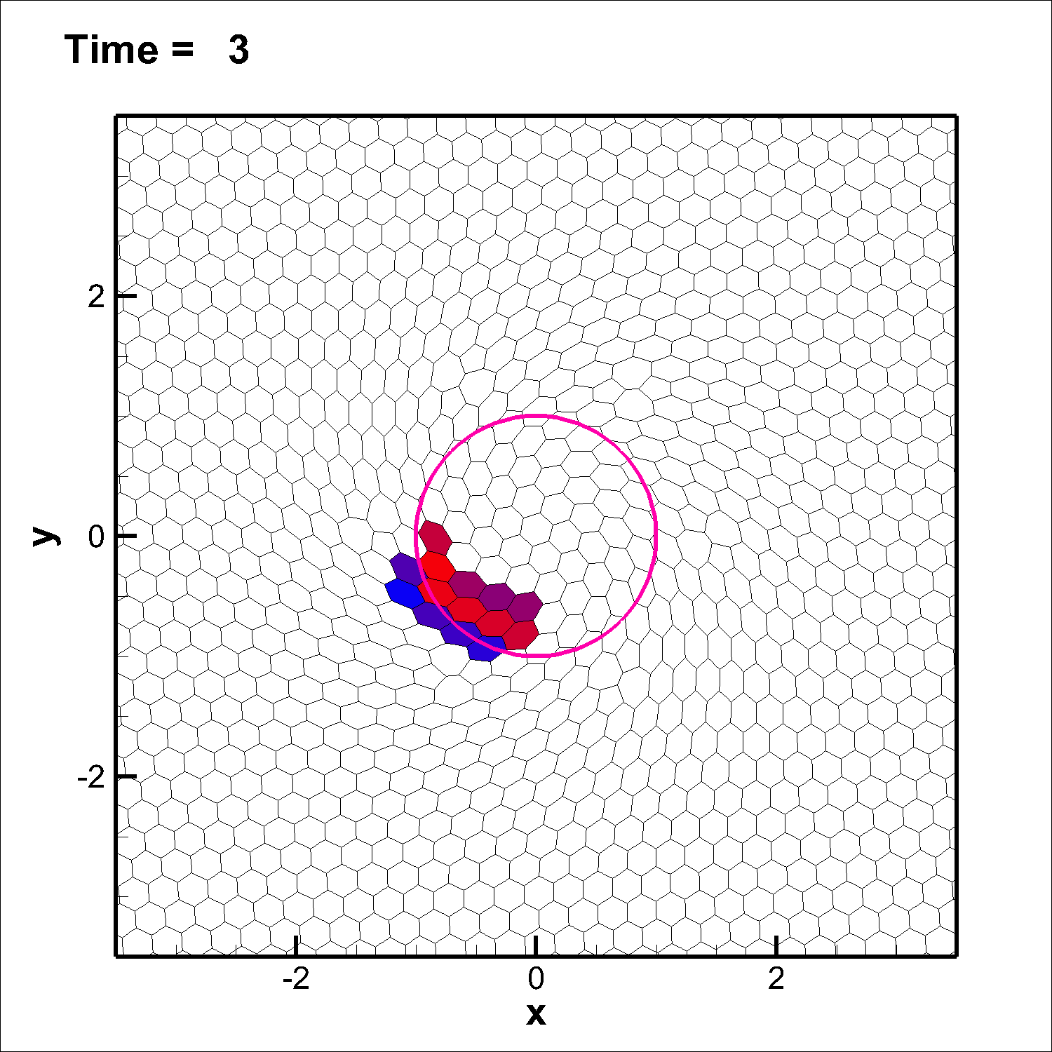 Figure 25
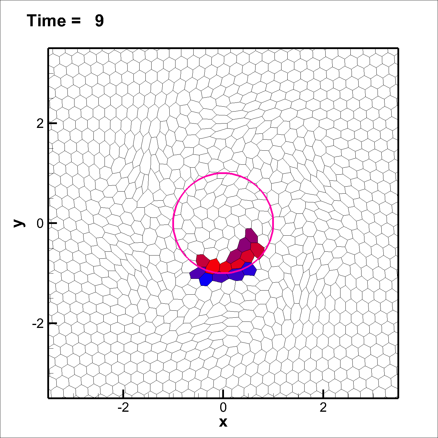 Figure 26
 Figure 27
 Figure 28
 Figure 29
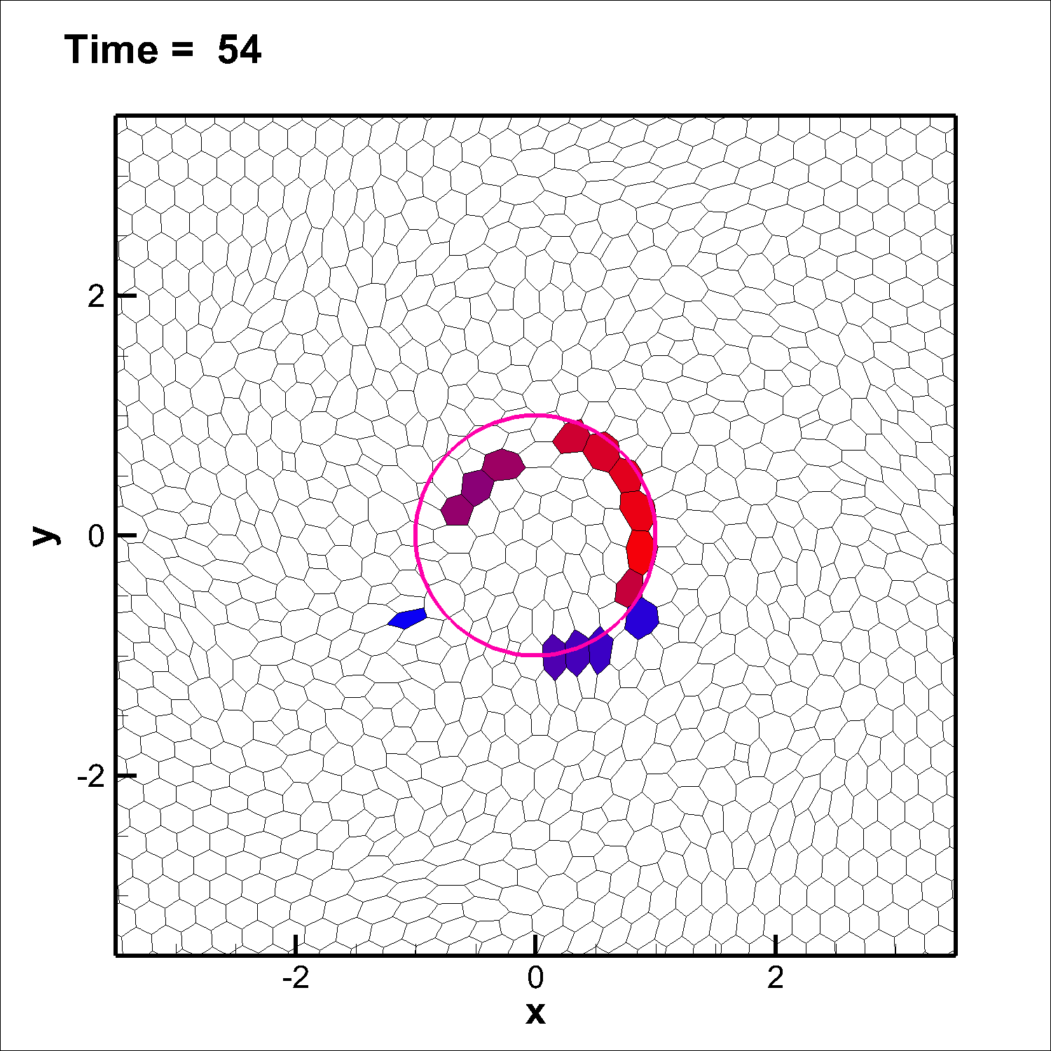 Figure 30
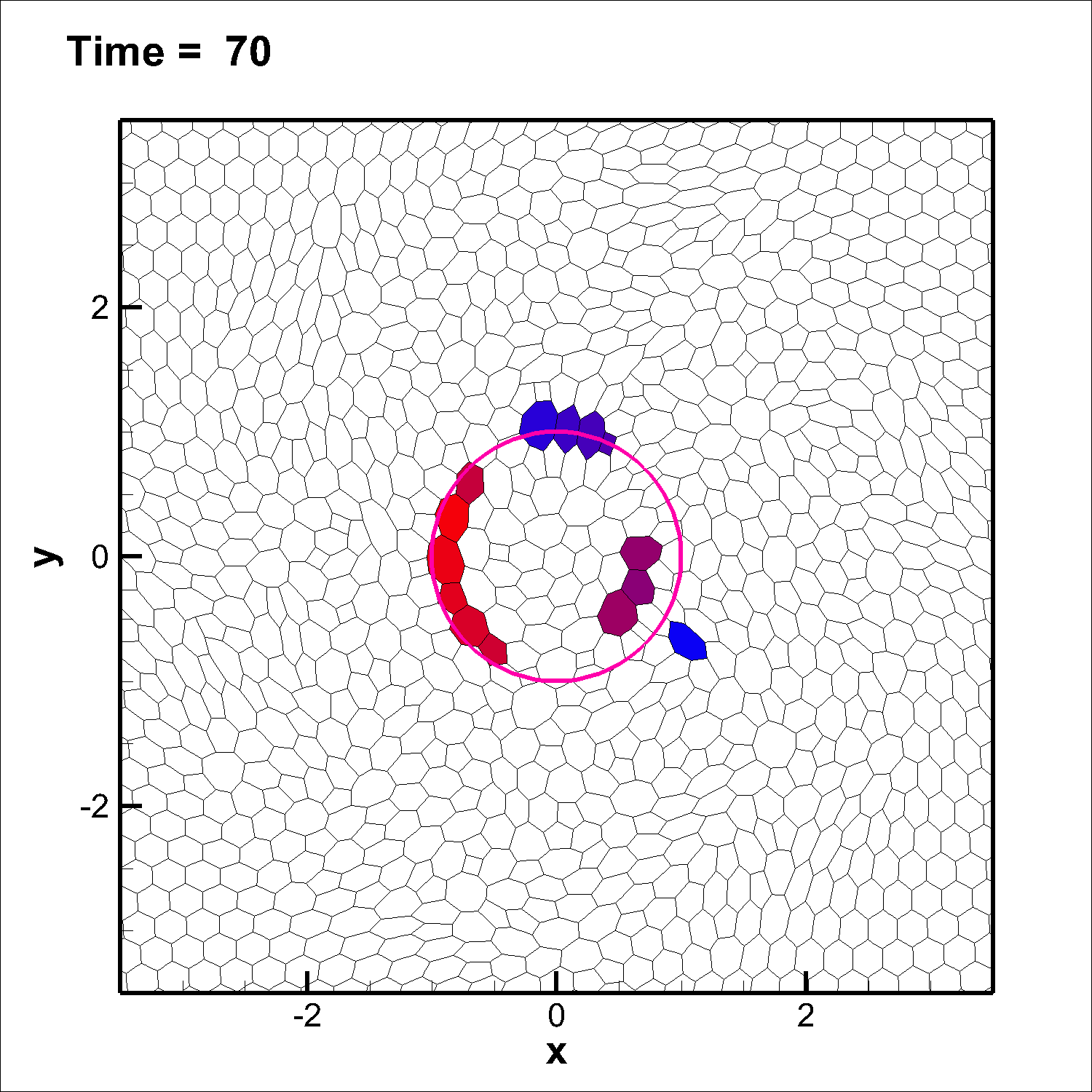 Figure 31
 Figure 32
 Figure 33
 Figure 34
 Figure 35
 Figure 36
 Figure 37
 Figure 38
 Figure 39
 Figure 40
| | | | | | | | | | | | |
|---|---|---|---|---|---|---|---|---|---|---|---|
| 3.8E-01 | 3.1E-02 | - | 3.8E-01 | 2.9E-02 | - | 1.9E-01 | 1.6E-03 | - | 4.7E-01 | 4.0E-02 | - |
| 2.0E-01 | 6.2E-03 | 2.4 | 1.9E-01 | 4.6E-03 | 2.8 | 1.3E-01 | 4.1E-04 | 3.4 | 3.8E-01 | 1.4E-02 | 4.8 |
| 1.3E-01 | 2.4E-03 | 2.4 | 1.3E-01 | 1.4E-03 | 2.9 | 9.9E-02 | 1.4E-04 | 3.8 | 1.3E-01 | 2.5E-04 | 3.8 |
| 9.9E-02 | 1.3E-03 | 2.3 | 9.9E-02 | 6.1E-04 | 3.0 | 7.9E-02 | 6.0E-05 | 3.9 | 9.9E-02 | 6.7E-05 | 4.6 |
| 8.0E-02 | 7.8E-04 | 2.2 | 7.9E-02 | 3.1E-04 | 2.0 | 6.7E-03 | 3.0E-05 | 3.8 | 7.9E-02 | 2.4E-05 | 4.7 |
| | | | | | | | | | | | |
|---|---|---|---|---|---|---|---|---|---|---|---|
| 7.5E-01 | 6.3E-03 | - | 7.5E-01 | 1.4E-02 | - | 6.1E-01 | 1.4E-03 | - | 1.4E-00 | 1.1E-02 | - |
| 6.1E-01 | 4.2E-04 | 1.9 | 6.1E-01 | 7.2E-03 | 3.4 | 5.2E-01 | 7.4E-04 | 3.7 | 1.0E-00 | 2.0E-03 | 5.9 |
| 3.2E-01 | 9.9E-04 | 2.2 | 3.2E-01 | 9.3E-04 | 3.2 | 4.7E-01 | 4.1E-04 | 5.9 | 9.8E-01 | 1.6E-03 | 4.7 |
| 2.2E-01 | 4.4E-04 | 2.0 | 2.2E-01 | 2.8E-04 | 3.0 | 3.2E-01 | 7.7E-05 | 4.4 | 8.9E-01 | 9.0E-04 | 5.9 |
| 1.6E-01 | 2.5E-05 | 2.0 | 1.6E-01 | 1.2E-04 | 3.0 | 2.2E-01 | 1.6E-05 | 4.0 | 8.5E-01 | 7.0E-04 | 5.1 |
| ordering from common neighbor | ||
|---|---|---|
| 0.319411631217116 | 9.2414523328907E-04 | - |
| 0.242212163540348 | 3.9353901580992E-04 | 3.1 |
| 0.194949032600822 | 2.0616099552666E-04 | 3.0 |
| 0.163155447483668 | 1.1964571728528E-04 | 3.1 |
| 0.122985013713313 | 5.1270456290057E-05 | 3.0 |
| ordering from common neighbor | ||
| 0.319411631217114 | 9.2414523328982E-04 | - |
| 0.242212163540348 | 3.9353901581037E-04 | 3.1 |
| 0.194949032600822 | 2.0616099552752E-04 | 3.0 |
| 0.163155447483668 | 1.1964571728459E-04 | 3.1 |
| 0.122985013713313 | 5.1270456288495E-05 | 3.0 |
| ordering from common neighbor | ||
| 0.319411631217116 | 9.2414523328907E-04 | - |
| 0.242212163540348 | 3.9353901580992E-04 | 3.1 |
| 0.194949032600822 | 2.0616099552666E-04 | 3.0 |
| 0.163155447483668 | 1.1964571728400E-04 | 3.1 |
| 0.122985013713313 | 5.1270456291299E-05 | 3.0 |
| Method | time steps | slivers | restarts | Mesh | standard | sliver |
|---|---|---|---|---|---|---|
| FV | 5524 | 21930 | 5 | 0.31 | 56.03 | 0.01 |
| FV | 4896 | 19819 | 4 | 0.31 | 56.00 | 0.01 |
| DG | 33019 | 19392 | 0 | 1.29 | 91.07 | 0.004 |
| DG | 55496 | 18995 | 2 | 0.25 | 96.31 | 0.001 |
| Method | time steps | slivers | restarts | Mesh | standard | sliver |
|---|---|---|---|---|---|---|
| FV | 150 | 1785 | 0 | 0.16 | 79.69 | 0.003 |
| DG | 883 | 2238 | 3 | 0.70 | 64.59 | 0.002 |
| Method | time steps | slivers | restarts | Mesh | standard | sliver |
|---|---|---|---|---|---|---|
| FV , | 15219 | 15956 | 0 | 1.00 | 74.19 | 9.7E-4 |
| DG , | 27951 | 2707 | 0 | 4.23 | 87.65 | 6.5E-4 |
| DG , | 54493 | 1297 | 0 | 0.65 | 95.64 | 9.0E-5 |
| DG , | 41919 | 17114 | 0 | 5.3 | 86.43 | 6.1E-4 |
| | | | | | | | | | | | |
|---|---|---|---|---|---|---|---|---|---|---|---|
| 4.6E-01 | 3.3E-02 | - | 3.2E-01 | 1.0E-02 | - | 4.7E-01 | 2.1E-02 | - | 6.0E-01 | 3.6E-0.2 | - |
| 3.9E-01 | 1.6E-02 | 1.8 | 2.4E-01 | 5.5E-03 | 2.3 | 3.2E-01 | 6.0E-03 | 3.2 | 5.8E-01 | 3.0E-0.2 | 5.8 |
| 2.4E-01 | 8.9E-03 | 2.3 | 1.9E-01 | 2.7E-03 | 3.3 | 2.4E-01 | 2.0E-03 | 3.9 | 5.6E-01 | 2.7E-0.2 | 3.6 |
| 1.9E-01 | 5.3E-03 | 2.4 | 1.6E-01 | 1.5E-03 | 3.1 | 2.2E-01 | 1.3E-03 | 3.6 | 5.5E-01 | 2.3E-0.2 | 5.9 |
| 1.6E-01 | 3.4E-03 | 2.5 | 1.4E-01 | 1.0E-03 | 2.9 | 1.9E-01 | 8.1E-04 | 4.8 | 5.2E-01 | 1.8E-0.2 | 4.8 |
| | | | | | | | | | | | |
|---|---|---|---|---|---|---|---|---|---|---|---|
| 4.7E-01 | 8.5E-03 | - | 6.1E-01 | 2.8E-03 | - | 8.8E-01 | 1.1E-03 | - | 1.6E-00 | 6.9E-0.3 | - |
| 3.2E-01 | 3.2E-04 | 2.5 | 4.7E-01 | 1.3E-03 | 2.8 | 7.5E-01 | 6.2E-04 | 3.5 | 6.1E-01 | 1.3E-0.4 | 4.1 |
| 2.8E-01 | 2.1E-04 | 2.9 | 3.8E-01 | 7.3E-04 | 2.7 | 6.1E-01 | 3.1E-04 | 3.4 | 5.2E-01 | 4.7E-0.5 | 5.8 |
| 2.4E-01 | 1.6E-04 | 2.0 | 3.5E-01 | 5.6E-04 | 3.6 | 5.5E-01 | 1.9E-04 | 4.3 | 4.9E-01 | 3.1E-0.5 | 8.1 |
| 1.9E-01 | 9.7E-05 | 2.4 | 3.2E-01 | 4.1E-04 | 3.0 | 3.2E-01 | 2.3E-05 | 3.9 | 4.7E-01 | 2.4E-0.5 | 5.3 |
Peer Reviews
No public reviews on file for this paper yet. If you reviewed it on a platform where reviews are public (OpenReview, ICLR, NeurIPS, ICML), you can paste yours below so the community can read it here.
Videos
No videos yet. Explain this paper in a talk, walkthrough, or lecture? Add one.
High order direct Arbitrary-Lagrangian-Eulerian schemes on moving Voronoi meshes with topology changes
Elena Gaburro*∗*
Walter Boscheri
Simone Chiocchetti
Christian Klingenberg
Volker Springel
Michael Dumbser
Department of Civil, Environmental and Mechanical Engineering, University of Trento, Via Mesiano 77, 38123 Trento, Italy
Department of Mathematics and Computer Science, University of Ferrara, via Machiavelli 30, 44121 Ferrara, Italy
Department of Mathematics at Würzburg University, Emil Fischer Str. 40, Würzburg, 97074, Germany
Max-Planck-Institut für Astrophysik, Karl-Schwarzschild-Str 1, D-85748 Garching, Germany
Abstract
We present a new family of very high order accurate direct Arbitrary-Lagrangian-Eulerian (ALE) Finite Volume (FV) and Discontinuous Galerkin (DG) schemes for the solution of nonlinear hyperbolic PDE systems on moving two-dimensional Voronoi meshes that are regenerated at each time step and which explicitly allow topology changes in time. The Voronoi tessellations are obtained from a set of generator points that move with the local fluid velocity. We employ an AREPO-type approach [168], which rapidly rebuilds a new high quality mesh exploiting the previous one, but rearranging the element shapes and neighbors in order to guarantee that the mesh evolution is robust even for vortex flows and for very long simulation times. The old and new Voronoi elements associated to the same generator point are connected in space–time to construct closed space–time control volumes, whose bottom and top faces may be polygons with a different number of sides. We also need to incorporate some degenerate space–time sliver elements, which are needed in order to fill the space–time holes that arise because of the topology changes in the mesh between time and time . The final ALE FV-DG scheme is obtained by a novel redesign of the high order accurate fully discrete direct ALE schemes of Boscheri and Dumbser [20, 22], which have been extended here to general moving Voronoi meshes and space–time sliver elements. Our new numerical scheme is based on the integration over arbitrary shaped closed space–time control volumes combined with a fully-discrete space–time conservation formulation of the governing hyperbolic PDE system. In this way the discrete solution is conservative and satisfies the geometric conservation law (GCL) by construction. Numerical convergence studies as well as a large set of benchmark problems for hydrodynamics and magnetohydrodynamics (MHD) demonstrate the accuracy and robustness of the proposed method. Our numerical results clearly show that the new combination of very high order schemes with regenerated meshes that allow topology changes in each time step lead to substantial improvements compared to direct ALE methods on moving conforming meshes without topology change.
keywords:
Arbitrary-Lagrangian-Eulerian (ALE) Finite Volume (FV) and Discontinuous Galerkin (DG) schemes , arbitrary high order in space and time , moving Voronoi tessellations with topology change , a posteriori sub-cell finite volume limiter , fully-discrete one-step ADER approach for hyperbolic PDE , compressible Euler and MHD equations
††journal: Journal of Computational Physics
1 Introduction
The aim of this work is to present a novel family of explicit arbitrary high order accurate direct ALE Finite Volume (FV) and Discontinuous Galerkin (DG) schemes on moving Voronoi meshes that are regenerated at each time-step and which consequently allow also topology changes of the computational grid during the time evolution of the PDE system. The main novelty lies in the use of a space–time conservation formulation of the governing PDE system over closed, non-overlapping space-time control volumes that are constructed from the moving, regenerated Voronoi meshes between time and time . On these closed space–time control volumes the governing equations are then directly integrated by means of a high order fully discrete one-step ADER method. To the best knowledge of the authors, this is the first time that a unified framework for arbitrary high order accurate explicit non-oscillatory direct ALE FV and DG schemes on moving Voronoi meshes is developed, with an embedded mesh generator that builds a new mesh with a different topology at each time step.
1.1 State of the art
Lagrangian algorithms [178, 12, 42, 55, 85, 139, 41, 166, 134] are characterized by a moving computational mesh displaced with a velocity chosen as close as possible to the local fluid velocity. In the Lagrangian description of the fluid, the nonlinear convective terms disappear and, as a consequence, Lagrangian schemes exhibit virtually no numerical dissipation at contact discontinuities and material interfaces. Therefore, the aim of these methods is to reduce the numerical dissipation errors due to the convective terms, so that contact discontinuities are sharply captured and material interfaces can be properly identified and tracked.
Lagrangian finite volume schemes [139, 58, 49, 158, 131, 135, 133, 132, 37, 38] have been developed for the solution of nonlinear hyperbolic systems of PDEs, using the conservation form of the equations based on the physically conserved quantities like mass, momentum and total energy. Higher order Lagrangian-type schemes have been introduced in [46, 118, 47], where high order of accuracy in space is achieved with the aid of an ENO/WENO reconstruction and Runge-Kutta time stepping guarantees high order time discretization as well. Contrarily to the cell-centered methods listed so far, where all variables are located at the cell center of the primal mesh, staggered Lagrangian schemes [125, 122, 126] define the velocity at the grid vertexes and the other variables at the cell center, hence avoiding the need of a nodal solver to compute the mesh velocity of the grid nodes.
Another option for the numerical solution of hyperbolic conservation laws is given by Discontinuous Galerkin [153] and Finite Element (FE) schemes [51, 52, 53], where the numerical solution is approximated by piecewise polynomials within each control volume. Robust Lagrangian DG schemes are presented in [101, 137, 119, 120] and they have been extended to third order for the first time in [84, 82, 83, 115], while high order FE methods applied to Lagrangian hydrodynamics and elasto-plasticity can be found in [142, 162, 64, 62, 63].
Although these schemes are widely used, a common problem that affects almost all Lagrangian methods is the severe mesh distortion or mesh tangling that happens in the presence of shear flows, which may even cause a breakdown of the computation. This is the reason which led to the development of so-called Arbitrary-Lagrangian-Eulerian (ALE) methods [158, 17, 110, 116, 107, 14, 10], where the mesh velocity can be chosen independently of the local fluid velocity and thus the grid nodes can be moved at an arbitrary velocity. Cell-centered indirect ALE schemes aim at improving the mesh quality and the overall scheme robustness by performing a purely Lagrangian phase with subsequent rezoning (mesh optimization) [181, 106, 89] and remapping [15], where the numerical solution defined on the old mesh is transferred onto the new grid. To overcome the problem of mesh tangling, sliding line techniques have also been proposed [40, 150, 108], which deal with moving nonconforming meshes, whose element sides can slide in order to accommodate the distortion induced by shear flows. A very effective implicit DG method for dealing with weakly compressible Navier-Stokes flows with moving boundaries, using a tetrahedralization of space-time, has been presented in [179]. For what concerns indirect ALE schemes, interesting techniques for handling the mesh motion have been introduced by the so-called Reconnection ALE (ReALE) algorithms [124, 123, 16, 36], where the rezoning phase allows for topology changes at each time step of the computation. There, moving Voronoi tessellations have been employed and the obtained numerical results demonstrate that the flow features that have been computed in the Lagrangian phase can be better preserved compared to standard indirect ALE methods. ReALE schemes have also proven to be particularly well suited for dealing with multimaterial fluid flows, in order to sharply capture the interfaces across different materials thanks to a conservative remapping phase which transfers the information from the old mesh to the newly generated one, which keeps tracking the interface. ReALE schemes can therefore be considered as the seminal works concerning moving mesh methods with topology changes.
Among the different approaches that have been presented in the literature (pure Lagrangian, indirect ALE based on rezoning and remapping, ReALE as well as special nonconforming slide line treatments), a novel family of methods has been proposed, so-called direct Arbitrary-Lagrangian-Eulerian (ALE) schemes. Also in the framework of direct ALE the mesh velocity can be chosen in an arbitrary way. Usually, it is chosen close to the local fluid velocity. However, the mesh quality can be optimized by a rezoning phase which takes place before the computation of the numerical fluxes, hence allowing the space-time control volumes to be defined for each computational cell by connecting the element configuration at the current time level to the next time level . Next, the mesh motion is taken into account directly in the numerical flux computation of the FV or DG scheme, without needing any remeshing plus remapping strategy. Furthermore, such approaches naturally extend to unstructured meshes in multiple space dimensions [18] and to slide line treatment with nonconforming meshes [88, 86]. Direct ALE schemes have been recently presented in [30, 19, 20, 22, 29] by employing either very high order FV and DG schemes, also in combination with time-accurate local time stepping (LTS), see [68, 24]. These works are characterized by a fixed mesh topology, which makes it impossible to study phenomena affected by strong shear motion and vortex flows for very long simulation times, since mesh tangling would inevitably occur and lead to a breakdown of the simulation before the final time is reached, unless strong mesh smoothing or relaxation procedures are introduced. Also, it should be remarked that other ways to prevent, or at least to remarkably postpone, the breakdown of simulations consist in employing high order curvilinear meshes, see the results published in [62, 10, 2, 3]. Moreover, notice that direct ALE schemes, even when constrained to a fixed connectivity, already ameliorate standard Lagrangian results for complex flow patterns.
From what was observed so far, the idea of allowing a change of topology at each time step within the direct ALE framework arises. A seminal work along this direction is represented by the AREPO code of Springel and collaborators [168, 169, 144, 145]. AREPO is a massively parallel second order accurate two- and three-dimensional direct ALE finite volume scheme on moving Voronoi tessellations that are rebuilt at each time step from a set of generator points which are moving with the local fluid velocity. The documented results obtained with the AREPO technique clearly highlight the robustness and potential of that approach. Similar work in the context of finite element schemes can be found in the well-known particle finite element method of Oñate and Idelsohn et al., see [98, 149, 141, 111, 99, 140]. In the above-mentioned references, the mesh is completely regenerated at each time step, thus naturally allowing for large deformations and strong shear flows without causing mesh tangling and highly distorted elements.
1.2 Challenges of this work
Up to now the AREPO algorithm [168, 169] is at most second order accurate in space and time. We therefore believe that its results can still be improved by (i) increasing the order of accuracy of the underlying FV scheme in both space and time and by (ii) introducing a higher order DG method into the AREPO framework. However, above all, the main difficulty arises from the fact that high order direct ALE schemes need a complete knowledge of the space–time connectivity between two consecutive time steps and , and not only of the spatial connectivity at each time level. Furthermore, if a change of connectivity is allowed, the space-time connectivity does not coincide neither with the connectivity at time , nor with the one at time . Hence, an automatic way to construct the missing space-time connectivity from the available spatial connectivities at and must be found. In addition, the space–time control volumes should be allowed to have as bottom and top faces polygons with a different number of edges, and, moreover, even degenerate space–time sliver elements must be incorporated in order to fill the space-time holes that are caused by the changing topology. With sliver elements we refer to space–time elements whose areas at time and are null, but whose space–time volume is not zero, see Sections 2.6 and 2.7. In other words, sliver elements exist only in the space-time volume strictly bounded between two consecutive time levels, therefore they must be taken into account only if the numerical scheme requires the full space-time connectivity.
Finally, this kind of elements should be not only built, but also the one-step ADER finite volume and DG schemes must be substantially modified to handle the integration of the PDE over these new types of space-time control volumes. A proof of concept that direct ALE methods can work even on degenerate space-time elements was already given in [88] for second order FV schemes on moving nonconforming meshes, but a much greater effort is necessary for dealing with such a general situation as the one treated in this work.
1.3 Structure of the paper
The rest of the paper is organized as follows. In Section 2 we first introduce our moving computational mesh, the data representation over it, and the reconstruction procedure needed to obtain high order in space. Next, in Section 2.4 we introduce the mesh motion strategy which is obtained by computing the new coordinates of a set of points (eventually with high order of accuracy, see Section 2.4.1) and re-drawing around them a new Voronoi tessellation, whose topology could differ from the previous one. Mesh optimization techniques (see Section 2.5) can be employed as well in order to improve the quality of the new tessellations.
Sections 2.6 and 2.7 represent the first key ingredient of our algorithm: we explain how to deal with the topology changes that are caused by the regeneration of the Voronoi tessellation at each time step. Then, we explain how to automatically construct the space–time connectivity and the space–time sliver elements.
Once this has been set up, in Section 3 we describe our direct ALE FV-DG scheme, namely an algorithm belonging to the class of direct ALE schemes [69], which allows us to formulate a Finite Volume (FV) and a Discontinuous Galerkin (DG) scheme within a unique framework. The method is first presented for standard moving Voronoi elements, i.e. Voronoi elements that are displaced without modifying their shape, i.e. the number of their nodes remains the same at each time level. Then, the method is extended to Voronoi elements with different bottom and top faces and finally to sliver elements in Sections 3.1.2 and 3.2.2, which is the second key ingredient of our scheme. In particular, for both types of elements we have detailed: i) the predictor step, which is essential for obtaining high order in time in a fully-discrete one-step procedure, ii) the corrector step, which allows the solution to be updated, and iii) the limiter that prevents spurious oscillations in the DG scheme.
Concerning a potential extension to compressible multi-material flows, the numerical approach proposed in this paper is obviously best suited for so-called diffuse interface models, such as the Baer-Nunziato model of compressible two-phase flows [5, 4], the Saurel-Abgrall model [159, 1, 160] or the compressible multi-phase model recently proposed by Romenski et al. [156, 155, 154].
In Section 4 we show a large set of numerical results, including convergence rates up to fifth order of accuracy in space and time for smooth problems, as well as a wide set of benchmark test cases solved with our ALE FV-DG schemes on moving Voronoi meshes with topology change for different systems of hyperbolic equations, namely the Euler equations of compressible gas dynamics, including the gravity source term, and the ideal MHD equations. The numerical results are commented and compared with available reference solutions wherever possible.
The paper is closed by some conclusive remarks and an outlook to future work in Section 5.
2 Numerical method I: handling a moving Voronoi tessellation with topology changes and data reconstruction
We consider a very general formulation of the governing equations in order to model a wide class of physical phenomena, namely all those which are described by equations that can be cast into the following form,
[TABLE]
where is the spatial position vector, represents the time, is the vector of conserved variables defined in the space of the admissible states , is the non linear flux tensor, and represents a non linear algebraic source term.
To discretize the moving two-dimensional domain we employ a centroid based Voronoi-type tessellation made of non overlapping polygons . The tessellation is first built at time and then it is regenerated at each time step . Data are represented via high order polynomials in each Voronoi polygon, which are either given by a (C)WENO reconstruction procedure for FV schemes, or are directly available from the numerical solution when a DG method is considered.
2.1 Computational grid
At time we fix the position of points, called generator points: their coordinates are denoted as and they are uniformly distributed inside the rectangular domain as well as on its boundary. Next, we build a Delaunay triangulation having these generators as vertexes of the triangles. The defining property of the Delaunay triangulation is that the circumcircle of each triangle is not allowed to contain any of the other generator points in its interior. This empty circumcircle property distinguishes the Delaunay triangulation from the many other triangulations of the plane that are possible for the point set. Furthermore, this condition uniquely determines the triangulation for points in general position (except for circles with more than three generator points on them for which the Delaunay triangulation contains degenerate cases where it may flip by an infinitesimal motion of one of the points). For this step we follow the Delaunay algorithm presented in [35, 180], where the point location phase is efficiently performed by employing a jump-and-walk method [138].
Each generator point is then associated to a centroid based Voronoi element by connecting counterclockwise the barycenters of all the Delaunay triangles having this generator point as a vertex. Note that the use of barycenters (instead of circumcenters) to construct these Voronoi-type elements avoids degenerate situations caused by the violation of the empty circumcircle property, thus it does not need to be resolved. We refer to Figure 1 for a graphical interpretation (generator points are always plotted in red and Voronoi vertexes in blue). In particular, given a Voronoi polygon we denote by the set of its Voronoi neighbors, by the set of its edges, and by the set of its vertexes, consistently ordered counterclockwise. Finally, the barycenter of a Voronoi polygon is noted as (note that usually it does not coincide with the generator point, and it is always plotted in orange). By connecting with each vertex of we subdivide the Voronoi polygon in subtriangles denoted as .
2.2 Spatial representation of the numerical solution
The numerical solution for the conserved quantities in (1) is represented via a cell-centered approach inside each Voronoi polygon at the current time by piecewise polynomials of degree denoted by and defined in the space ,
[TABLE]
where are modal spatial basis functions used to span the space of polynomials up to degree . In the rest of the paper we will use classical tensor index notation based on the Einstein summation convention, which implies summation over two equal indices. The total number of expansion coefficients (degrees of freedom, DOFs) for the basis functions depends on the polynomial degree and is given by , with
[TABLE]
where in this paper, since we are dealing only with two-dimensional domains. As basis functions in (2) we employ a Taylor series of degree in the variables directly defined on the physical element , expanded about its current barycenter and normalized by its current characteristic length
[TABLE]
being the radius of the circumcircle of . The unknown expansion coefficients in (2) are the rescaled derivatives of the Taylor expansion about . The time dependence of derives from the time-dependence of the cell barycenter .
The discontinuous finite element data representation (2) leads naturally to both a Discontinuous Galerkin (DG) scheme if , but also to a Finite Volume (FV) scheme in the case . This indeed means that for we have , with and (2) reduces to the classical piecewise constant data representation that is typical of finite volume schemes:
[TABLE]
Here, the only degree of freedom per element is the usual cell average . Note also that in the case the representation given by (2) already provides a spatially high order accurate data representation with accuracy , which is not the case when . If we are interested in increasing the spatial order of accuracy of a finite volume scheme, up to for example, we need to perform a spatial reconstruction that generates a spatially high order accurate reconstruction polynomial of degree (see the CWENO procedure presented in 2.3) that reads
[TABLE]
where we simply employ the same basis functions for the reconstruction according to (4), but with rather than , see also [69].
With this notation, our method falls within the more general class of schemes introduced in [69] for fixed unstructured simplex meshes in two and three space dimensions. In [69, 65, 128, 129] a new family of hybrid, reconstructed discontinuous Galerkin methods was proposed, in which a Hermite-type reconstruction of degree is performed on cell data represented by polynomials of degree . In this paper, however, we restrict ourselves to the two most common situations: (i) , with arbitrary high order reconstruction of degree , which indeed corresponds to a FV scheme of order , and (ii) , which corresponds to a DG scheme of accuracy . Within the general formalism one can simultaneously deal with arbitrary high order FV and DG schemes inside a unified framework, with only very few differences between the two schemes.
For the sake of uniform notation, when and hence , we trivially impose that the reconstruction polynomial is given by the DG polynomial, i.e. , which automatically implies that in the case the reconstruction operator is simply the identity.
2.3 CWENO reconstruction
For finite volume schemes () the reconstruction procedure allows us to compute a high order non-oscillatory polynomial representation of the solution for each Voronoi polygon , starting from the values of in and its neighbors. It should be employed in the case . As already stated above, the total number of unknown degrees of freedom is , with denoting the degree of the reconstruction polynomial .
In order to achieve high accuracy, a large stencil centered in is required, but this choice produces oscillations close to discontinuities, the well-known Gibbs phenomenon. Indeed, for linear reconstruction operators, the requirements of high order of accuracy and non-oscillatory behavior are in contrast with each other, due to the well-known Godunov theorem [90]. In order to fulfill also the requirement of non-oscillatory behavior, a nonlinear reconstruction operator has to be adopted. In this paper we rely on the CWENO reconstruction strategy first introduced in [112, 113, 114], and which can be cast in the general framework described in [50]. Here, we closely follow the work outlined in [79] for unstructured triangular and tetrahedral meshes. For the sake of completeness, we report here the entire algorithm: the differences with respect to [79] are highlighted in the last paragraph of this section.
The reconstruction starts from the computation of a so-called central polynomial of degree . In order to define in a robust manner, following [79, 11, 104, 164], we consider a stencil which is filled with a total number of elements, containing cell and its neighbors
[TABLE]
with the safety factor . Stencil includes the current Voronoi polygon , the first layer of Voronoi neighbors (node neighbors of ) denoted by , and is filled by recursively adding neighbors of elements that have been already selected, until the desired number is reached. The polynomial is then defined by imposing that its average on each cell matches the known cell average . Since , this of course leads to an overdetermined linear system, which is solved using a constrained least-squares technique (CLSQ) [72] as
[TABLE]
where is the set of all polynomials of degree at most . In other words, the polynomial has exactly the cell average on the polygon and matches all the other cell averages of the remaining stencil elements in the least-square sense. The polynomial is expressed in terms of the basis functions (4) of degree , hence
[TABLE]
and the integrals appearing in (8) are computed in each Voronoi polygon by summing the contribution of each of its sub-triangles . On the sub-triangles we employ quadrature points defined by the conical product of the one-dimensional Gauss-Jacobi formula, see [170].
To make the reconstruction operator nonlinear, which is required in the presence of shock waves, the CWENO algorithm makes use of other polynomials of lower degree. Given a Voronoi polygon with Voronoi neighbors , we construct interpolating polynomials of degree referred to as sectorial polynomials. More precisely, we consider stencils with , each of them containing exactly cells. Each includes always the central cell and two consecutive neighbors belonging to . An example of stencils and for a polygon with and is reported in Figure 2.
For each stencil we compute a linear polynomial by solving the reconstruction systems
[TABLE]
which are not overdetermined and therefore have a unique solution for non-degenerate locations of the Voronoi barycenters. Following the general framework introduced in [50], we select a set of positive coefficients such that
[TABLE]
and we define a new polynomial
[TABLE]
so that the linear combination of the polynomials with the coefficients is equal to and conservation is ensured. Specifically, we consider the linear weights used in [73], namely for and for the sectorial stencils. These weights are later normalized in order to sum to unity, according to the requirement (11). Finally, the sectorial polynomials with are nonlinearly hybridized with , as it is done also in other WENO schemes [102, 97, 8]. We thus obtain in as
[TABLE]
where the normalized nonlinear weights are given by
[TABLE]
In the above expression the non-normalized weights depend on the linear weights and the oscillation indicators with the parameters and chosen according to [72]. Note that in smooth areas, and then , so that we recover optimal accuracy. On the other hand, close to a discontinuity, and some of the low degree polynomials would be oscillatory and have high oscillation indicators, leading to and in these cases only lower order non-oscillatory data are employed in , guaranteeing the non-oscillatory property of the reconstruction. The oscillation indicators appearing in (14) are simply given by
[TABLE]
The CWENO procedure adopted in this work is similar to the one presented in [79] and it has been adapted to Voronoi polygons and their connectivity. The needed modifications concern the computation of integrals in (8), the number of sectorial polynomials, and the fact that basis functions are rescaled Taylor monomials referred to the physical element and not to the reference element, hence yielding a different and very simple evaluation of the oscillation indicators (15).
2.4 Evolution of the computational domain
At this point we have a high order spatial representation of the solution at the current time given by the polynomial of degree . We recall that if then ; if instead then is obtained through the reconstruction procedure described in the previous Section 2.3.
By evaluating at the generator points , i.e. with (6), we recover the local fluid velocity , that can be used to compute the new coordinates of the generator points simply as
[TABLE]
Note that in our ALE formalism, the mesh can be moved with any velocity, hence it is not necessary to always integrate the above relation (16) with high order of accuracy. Moreover, for the sake of simplicity, all along this manuscript we do not move boundary elements.
The Delaunay triangulation connecting the new coordinates of the generator points is now recomputed, as well as the corresponding updated Voronoi tessellation. Note that the only connection between the tessellations at time and is the number of generator points (i.e. of Voronoi polygons) and their global numbering. Instead, the shape of each polygon is allowed to change, i.e. , and consequently also the connectivities, i.e. for example .
This change of the grid topology is actually the strength of the present algorithm, since it allows us to maintain a high mesh quality without distorted elements, as depicted in Figures 7 and 9, where we show a comparison between the results obtained by allowing topology changes and by imposing a fixed connectivity, respectively. However, more care is needed in order to update the solution from time to . In particular, to obtain a high order direct ALE scheme we need a complete knowledge of the space–time structure between the two time levels, i.e. we need to construct the so called space–time control volumes and their space–time connectivity. We would like to emphasize that up to Finite Volume schemes of order , one could avoid the procedure that we are going to introduce (see [168, 145]), but starting from order it is essential.
2.4.1 High order integration of the trajectories of the generator points
Due to the ALE framework of the present work, the mesh can in principle be moved with an arbitrary velocity, and there is not a specific necessity of moving the grid in a fully Lagrangian fashion. Nevertheless, (16) can also be replaced by a high order Taylor method [23, 32, 171], leading to a high order approximation of the Lagrangian trajectories of the generators points. The use of this technique for example improves mesh quality in vortex flow, as clearly shown in Section 4.1.1, and also improves the overall Lagrangian behavior of the algorithm.
In what follows we detail the high order approach used for the integration of the flow trajectories.
The Taylor expansion of the new position of a generator point at time with respect to its position at time can be written as
[TABLE]
which achieves fourth order of accuracy in time. Now, the high order time derivatives in (17) are replaced by high order spatial derivatives, via the Cauchy-Kovalevskaya procedure, using repeatedly the trajectory equation
[TABLE]
and assuming a stationary velocity field (i.e. ), hence
[TABLE]
The chain rule, as written in (19), can be applied iteratively to obtain the third derivative of the position
[TABLE]
and similarly, the fourth derivative reads
[TABLE]
Finally, the partial derivatives of are recovered from the local fluid velocities through the high order polynomials (6) which represent the conserved variables inside each cell with high order of accuracy. Since is given via modal basis functions, the coefficients already represent the values of the partial derivatives with respect to of the conserved variables, if a sufficiently high order accurate method is employed. Then, the chain rule should be applied in order to recover the partial derivatives of the primitive variable from those of the conserved variables and .
2.5 Mesh optimization
The ALE framework also allows to apply some mesh optimization techniques, since the mesh velocity is not constrained to follow the local fluid velocity exactly. Furthermore, an additional level of liberty in the choice of type of smoothing scheme is introduced by the possibility of changing the grid connectivity between consecutive time levels. In this work, the mesh optimization methods are implemented by slightly modifying, at each time step, the motion of the Voronoi generator points (that is, the vertexes of the dual Delaunay triangulation). This aims at improving the overall robustness of the method, as well as reducing numerical errors and spurious mesh imprinting.
In general, the target polygonal elements will have a locally uniform edge length (i.e. no small edges for a given element, smoothly graded mesh size) and will not be excessively stretched in one direction only, so that anisotropies due to differences in numerical diffusion are minimized. More importantly, this increases the robustness of the matrix computations involved in the polynomial data reconstruction and in the fully discrete update formulae. Also, we must note that these objectives shall be pursued in conjunction with the interest of preserving an accurate mesh motion that follows the local flow field, maintaining the Lagrangian character of the numerical method as far as possible. This means that one must allow a certain degree of anisotropy in the mesh, which might be desirable to resolve flow discontinuities or strong gradients.
The mesh regularization procedure begins by computing all the new positions for the generator points of the Voronoi grid and then recovering, for each generator, the position that is prescribed by a simple smoothing technique applied to the candidate positions . We say that is a location for the generator that is optimal in the sense of mesh quality, as opposed to optimal in following the flow of the fluid, which would be the role taken by . The candidate position is subsequently replaced by a corrected value that is given by the weighted average , with being a blending factor that yields the balance between the amount of mesh motion due to fluid flow with the one due to smoothing.
Concerning the determination of , we decided to simply compute it from the application to of one iteration of a Lloyd-type algorithm; that is, after updating the Delaunay triangulation of the generator points taking into account their new candidate positions , we evaluate the quality-optimal position for generator as
[TABLE]
We define to indicate the set of Delaunay triangles that share as a vertex, while we denote with and the other two vertexes of the triangle , that is, the two that do not coincide with . The choice of weights yields different smoothing methods, and in this work we mainly employ to obtain an algorithm that is reminiscent of Lloyd smoothing [121], as this would prescribe that each generator shall be moved to the centroid of the polygonal chain obtained by connecting all vertexes and of all Delaunay triangles in . This choice tends to eliminate small edges just like the algorithms forwarded in [165, 33, 147]. Alternatively, we can set and obtain Laplacian smoothing [94, 81], that is, the generic generator is moved to the center of mass of the system of point masses defined by the vertexes of the above described polygonal chain. Laplacian smoothing yields nicely rounded cells and tends to preserve the grading of the mesh.
Once a set of quality-aware node positions has been determined, the algorithm must choose how to compromise between such positions and those prescribed by the fluid motion. Instead of simply fixing the value of as a simulation parameter, we chose to let vary with time by recomputing it as a function of the solution data and of the current grid configuration, as well as by accounting for the specific explicit time step restriction in use. Specifically, we compute the relaxation parameter as
[TABLE]
with being a rough scaling estimate for the fluid velocity, computed at each time step as the maximum velocity encountered for all generator points, the time step size, and an indicator for the mesh spacing, given by the minimum value of the ratio between the area and the perimeter of all Voronoi polygons, in analogy to how the time step duration is determined in (25). The underlying idea is that we want to balance, during each time step, the spatial scaling of fluid flow, with a characteristic length representative of the mesh motion due to pure smoothing in the smallest cells of the domain, which we implicitly assume to be the most delicate. In this way, we have replaced the blending factor with another non-dimensional smoothing parameter , that fixes the strength of smoothing in the small cells that are those that might otherwise compromise the stability of the computation. The square root is arbitrarily introduced in order to reduce the sensitivity of Equation (23) to sudden variations in the flow speed .
Note that, although in a very approximate form, the formula (23) scales with the square root of a characteristic Mach number, at least when is negligible with respect to sound speed or vice versa; one can verify this by substituting (25) in (23) and noting that it simplifies into an expression that includes the degree of the polynomial data , the CFL coefficient, and an approximate Mach number. Further investigations on more complex scaling expressions that correct for such residual dependencies, as well as space-dependent formulae, are left for future work.
The results presented in this paper are obtained by moving the generators with the local fluid velocity and by applying one of the smoothing techniques described here, with different values of the smoothing parameter .
2.6 Space–time connectivity
For the sake of clarity, let us first consider the simple case in which no topology changes have occurred between and , i.e. and , as illustrated in Figure 3. Here, the space–time control volume is easily obtained by connecting each node of the polygon via straight line segments with the corresponding node of . Moreover, each sub–triangle is connected with the corresponding obtaining a sub–space–time control volume, denoted by in the following, which has the form of an oblique prism in space–time, with triangular faces on the bottom () and the top ().
We underline that each space–time element is given by a volume that is closed by the polygon at time , the polygon at and by the lateral space-time faces which are quadrilaterals in space–time and represent the time evolution of the edges . Here, denotes the number of space–time neighbors of . The total surface of is denoted with
[TABLE]
Technical details 1
We recall that the node numbering (i.e. the numbering of the blue points in Figure 3) could be in principle different at the two time levels so the correspondence between the nodes at time level and is not obvious. Nevertheless, it can be recovered from the numbering of the Voronoi neighbors that on the contrary remains the same. Therefore, we loop over , we find the edges shared between and , and we put in correspondence their end points, so that the space–time control volume can be defined. Besides, the surface obtained by connecting the end points of and is noted as , see Figure 6b.
Let us now consider and in the case . Now, the space–time connection between them induces the appearance of degenerate elements of two types: (i) degenerate sub–space–time control volumes , where either their top or bottom faces are degenerate triangles that are collapsed just to a line, see Figures 4b-4c; (ii) and also sliver space–time elements, see Figure 4d. Technical details on their construction (intended for the reader interested in reproducing the algorithm) are reported in the following paragraph. The main characteristics of this kind of elements are described in next Section 2.7.
Technical details 2
First, we order and starting from the first common neighbor (evidence that this choice does not affect the results are shown in Table 3). Then, we merge the two set of neighbors to compute which, in this case, does not coincide neither with nor with . contains all the polygons of and counted once (i.e. without multiple entries) and counterclockwise ordered respecting the order of both and . It represents the set of space–time neighbors of .
Next, we have to find the node connections in order to build , which are not obviously determined and are recovered from . We loop on (this loop assures that we account for all the nodes of , since by considering all the neighbors we also consider all the edges of both and ) and we proceed as follows:
- I.
If belongs both to and to , the node connection procedure falls into the previous one, and a standard and can be recovered by connecting the end points of the edges shared between and . Referring to depicted in Figure 4, we could fix as first common neighbor because and : nodes and can be easily connected.
- II.
If but , then the end points of the edge shared between will be connected to a unique node at time , namely the top node which is common to and at time . Referring to Figure 4, both nodes and will be connected with node . In this case , is degenerate: it does not have a rectangular shape but a triangular one. Also is degenerate because its top face is just given by a line connecting the barycenter of with the common top node (node in Figure 4).
- III.
If but , then the end points of the edge shared between will be connected to a unique node at time , namely the bottom node which is common to and at time . Referring to shown in Figure 4, both nodes and will be connected with node . As in the previous case, has a degenerate triangular shape and also is degenerate because its bottom face is just given by a line connecting the barycenter of with the common bottom node (node in Figure 4).
Note that when a change of topology occurs in a Voronoi polygon, the same happens to three of its neighbors and a total of four degenerate sub–space–time control volumes will be originated, two of type (II) and two of type (III), refer to Figures 4b-4c. Moreover, a void is left between them: to fill it and recover a fully conservative discretization, we insert a new element called space–time sliver element, depicted in Figure 4d, whose bottom and top faces just coincide with an edge of the tessellation at time and , respectively. We denote this kind of element with , its total lateral surface with and each of the four lateral faces with .
Technical details 3
The nodes of a sliver element are given by the end points of those edges that flip between the two time steps and are ordered in such a way that the volume of is positive. Let us consider case (II) in which but : the edge between is taken as bottom face for the sliver. Then, we loop over the edges outgoing from the common top node: two of them belong to , the third one will be taken as top face of the sliver element. If that edge connects then one sliver element is enough to fill the space–time hole left from the topology change.
If this is not the case, as illustrated in Figures 5b-5d, more consecutive sliver elements will be necessary to fill the space–time holes. These consecutive sliver elements have the bottom face in common, given by the edge between , and the top faces given respectively by the edges composing the path connecting . A similar procedure is employed for situations depicted in Figures 5a-5c, corresponding to case (III). We allow a maximum of three consecutive sliver elements.
Two problems can arise while assembling the space–time connectivity: could be not sortable respecting both the order of and , or more than three sliver elements could be necessary to complete the connection path. In this case a MOOD [31, 25] procedure described in Section 3.4 will be adopted.
2.7 Degenerate sub–space–time control volumes and sliver space–time elements
The change of topology induces the appearance of degenerate elements in the space–time connectivity.
As is evident from Figures 4b-4c, some of the sub–space–time control volumes of , are triangular prisms with one of their top or bottom faces collapsed to just a line, and with the lateral space–time surface being of triangular shape (instead of the standard quadrilateral shape). They do not pose particular problems because they are part of a standard control volume, so everything is naturally well defined on them (basis functions, quadrature points, values of the numerical solution , of the reconstruction polynomials , and of the space–time predictor defined below in (26)).
On the contrary, the space–time sliver element in Figure 4d is a completely new control volume which does neither exist at time , nor at time , since it coincides with an edge of the tessellation at the old and at the new time levels, and, as such, has zero area in space at and . However, it has a non-negligible volume in space–time. The difficulties related to this kind of elements are due to the fact that is not clearly defined for them at time and that contributions across them should not be lost at time , in order to ensure conservation. Space–time sliver elements always have four neighbors, namely the two Voronoi polygons that share their degenerate bottom face (edge) and the two Voronoi polygons that share their degenerate top face (edge).
Note that the computation of numerical fluxes across degenerate triangular space–time faces has already been treated in [88]. In the same paper a proof of concept was given, that situations like those shown in Figures 4b-4c could be handled up to second order of accuracy. Instead, the treatment of sliver elements is a completely new topic.
3 Numerical method II: high order fully-discrete direct ALE FV-DG scheme
The governing equations (1) are now solved with the aid of a high order fully-discrete one-step predictor-corrector ADER FV-DG method obtained by generalizing the scheme first presented in [69] to our moving Voronoi meshes with topology change. ADER finite volume schemes go back to the pioneering work of Toro and Titarev [173, 177, 174, 161, 175] on approximate solvers for the generalized Riemann problem (GPR). ADER schemes have been originally developed in the Eulerian framework on fixed grids [173, 177, 174, 161, 175, 70, 39] and have subsequently also been extended to moving meshes in the ALE context [29, 20, 18, 21].
We recall that high order of accuracy in space is provided by the piecewise polynomial data representation , which for coincides with the DG polynomial, i.e. , while, in the Finite Volume case (), is obtained through the reconstruction procedure described in Section 2.3. In any case, only depends on the mesh configuration at time , so that an eventual degeneracy of the space–time geometry does not affect this first step.
Then, the predictor step consists in a local solution of the governing PDE (1) in the small, see [93], inside each space-time element , thus including the sliver elements . It is called local because it is obtained by only considering cell with initial data on , the governing equations (1) and the geometry of , without taking into account any interaction between and its neighbors. It provides, for each space–time control volume , a polynomial data representation (see below for the details) of high order both in space and time, which serves as a predictor solution, only valid inside , to be used for evaluating the numerical fluxes and sources when integrating the PDE in the final corrector step of the ADER scheme.
Lastly, the corrector step integrates the weak form of the PDE over the space-time control volumes , making use of the predictor solution , and returns by taking care of the coupling with neighbors through the numerical flux computations across . It ensures high order of accuracy in space and time, provided the high order of accuracy of . The scheme is by construction conservative since it takes into account all the flux contributions over , including those across the sliver elements (see Section 3.2.2). Moreover, the method is stable if the time-step size satisfies an explicit CFL stability condition, which reads
[TABLE]
In the above formula, is the length of the edge of and is the spectral radius of the Jacobian of the flux . On unstructured meshes the CFL stability condition requires the inequality to be satisfied, see [69].
3.1 High order in time: space–time predictor
In what follows, a predictor of the solution is recovered, which is valid locally inside and is given by high order piecewise space-time polynomials of degree that are expressed as
[TABLE]
with being a modal space–time basis of the polynomials of degree in dimensions ( space dimensions plus time), which read
[TABLE]
These basis functions are redefined at the beginning of each time step in function of the current position , thus they are directly linked to the current mesh configuration; however, contrarily to the test functions of Equation (37) that are used in the corrector step (see the next section), there is no need to move them during each time step, since they allow to represent information at the predictor step, which is only valid locally inside each .
The predictor is computed through an iterative procedure that looks for the polynomial satisfying a weak form of (1) obtained for any control volume as follows. We multiply the governing PDE (1) by a test function , integrate over and insert the discrete solution instead of , hence obtaining
[TABLE]
Differently from what has been proposed in [69, 70, 19, 20], here we do not integrate the first term in (28) by parts in time. Instead, we take into account potential jumps of on the boundaries of in the sense of distributions, combined with upwinding of the fluxes in time. This approach is similar to the path-conservative schemes proposed in [146, 44, 43], but much simpler, since the test functions are only taken from within and there is no need to define a non-conservative product on . Therefore, the integral containing the time derivative in (28) is rewritten as
[TABLE]
where denotes the interior of . Here, and denote the boundary-extrapolated inner and outer states across the jump on . Furthermore, are only those outward pointing unit-normal vectors on that point back in time and is their time component, i.e. . Upwinding in time is therefore automatically guaranteed, since we only consider the contributions coming from the past, according to the causality principle. In other words, only time fluxes that enter the space–time control volume contribute to the jump term in (29), and they are easily identified by checking the sign of the time component of the space–time normal vector .
3.1.1 Space–time predictor on standard space–time elements
For standard elements, we apply the jump term only on the bottom surface of the space–time element under consideration, where it then simplifies to
[TABLE]
with being simply given by the reconstruction polynomial at time and obviously on and thus . In this case, (29) reduces to
[TABLE]
for standard space–time elements. The reason for this choice is that in this manner, all space–time predictors of the standard elements are decoupled from each other, since they only require the initial data and no information from the neighbor elements. This will not be the case for sliver elements, for which we do not have any reconstruction polynomial available at . If we considered the jump terms also on lateral surfaces of standard space–time elements, the space–time predictors would no longer be independent of each other, since our mesh is moving and there will be in general always a non–empty subset of with . This would require a proper ordering of the execution sequence of the space–time predictors on the standard elements, but this is something we want to avoid. With the following definitions
[TABLE]
the weak form (28)-(29) can be compactly rewritten as
[TABLE]
where and contain all the expansion coefficients of in (26) and in (6), respectively. The solution of (33) can be found via a simple and fast converging fixed point iteration (a discrete Picard iteration), as detailed in [69, 95]. Here, as initial guess we simply impose for the common spatial degrees of freedom (with ) and zero for the other ones. For linear homogeneous systems, the discrete Picard iteration converges in a finite number of at most steps, since the involved iteration matrix is nilpotent, see [100]. In the nonlinear case we allow a maximum of iterations if convergence is not reached before, being iterations enough for obtaining the correct order of convergence.
Notice again that in (31) and therefore in (33) we have considered only one jump term, namely the contribution coming from the past through the bottom face of , where is known and well defined. This allows us to couple (28) with the initial condition via (31). No other information (as neighbors values) is taken into account in this local phase. Indeed, neighbor data will be considered later in the corrector step (Section 3.2).
The integrals above are evaluated using multidimensional Gaussian quadrature rules of suitable order of accuracy, see [170] and Figure 6 for details. In order to carry out the integration, we split the space-time volume into a set of sub–space-time volumes of , whose shape is an oblique triangular prism. Note that for degenerate sub–space–time control volumes, as those of Figures 4b and 4c, the above quadrature formulae remain well defined, hence the predictor procedure over them does not pose any problem and does not need any adaptation.
We emphasize that we first carry out the space–time predictor for all standard elements, which can be computed independently of each other, and only subsequently process the remaining space–time sliver elements. The reason for this will become clear in the next section.
3.1.2 Space–time predictor on the space–time sliver elements
The predictor procedure on space–time sliver elements, as those shown in Figures 4d and 5, needs particular care. The main problem connected with the space–time sliver elements is the fact that their bottom face is degenerate and consists only in a line segment, hence the spatial integral over vanishes, i.e. there is no possibility to introduce the initial condition of the local Cauchy problem at time into the predictor for space–time sliver elements.
Furthermore, the degenerate bottom faces are the edges of the Voronoi tesselation at and are thus at the interface between two adjacent elements, which have in principle a discontinuous solution . Therefore, an initial value for a sliver element is in general not easy to define. Thus, in order to couple (28) with some known data from the past we have to slightly modify the algorithm detailed previously.
In particular, the upwinding in time approach is not only used for the surface , as done in (30), but we actually use the jump terms on the entire part of the space–time surface that closes a sliver control volume. As already stated in the previous section, the information needed to feed the predictor is allowed to come only from the past, i.e. only from those space–time neighbors whose common surface exhibits a negative time component of the outward pointing space–time normal vector (). In this way, we can introduce information from the past into the space–time sliver elements by considering also its neighbor elements, but respecting at the same time the causality principle in time, hence using again upwinding for the flux evaluation of the jump term in (29). As a consequence, the predictor solution is again obtained by means of (28), but treating the entire space–time surface with the upwind in time approach, hence leading to
[TABLE]
where the following definitions for the sliver element hold
[TABLE]
This is slightly different from what is done for standard elements in (33), where only the space–time surface at time , i.e. , is considered for introducing the initial condition . Here, the information from the past comes through the upwind fluxes contained in the term in (34) and thus requires the knowledge of the predictor solution in the neighbor . This is the reason why the predictor step must first be performed over all the standard elements using (33), so that the predictor solution is always available to feed the temporal fluxes with the quantities that are needed for solving (34) in the case of the space–time sliver elements. We underline again that a space–time sliver element has always four standard Voronoi elements as neighbors. This closes the description of the predictor step for the space–time sliver elements.
3.2 Corrector step: direct ALE FV-DG scheme
This section contains the core of our direct ALE FV-DG scheme used to solve (1) on regenerating moving meshes.
Following [19, 20, 21], the PDE system (1) is rewritten in a space-time divergence form as
[TABLE]
with denoting the space-time divergence operator and being the corresponding space-time flux tensor. Then, we multiply (36) by a set of moving spatial modal test functions , which coincide with (4) at and at , i.e. and . The test functions are tied to the motion of the barycenter and move together with in such a way that at time they refer to the new barycenter . Thus, the test functions explicitly read as follows:
[TABLE]
These moving modal basis functions are essential for the approach presented in this paper. They naturally allow for topology changes, without the need of any remapping steps, which we want to avoid in a direct ALE formulation.
Next, integration over the closed space-time control volume yields
[TABLE]
Application of the Gauss theorem leads to the following weak form that is the basis of our fully-discrete ALE scheme
[TABLE]
where denotes the outward pointing space-time unit normal vector on the space-time faces composing the boundary of the space-time control volume. Moreover, the surface integral can be decomposed over the faces of given by (24).
3.2.1 Corrector step for standard space–time elements
We first describe the corrector step for standard space–time control volumes. After introducing the discrete solution , the space–time predictor and a two-point numerical flux function on the element boundaries of the type
[TABLE]
into (39), where and are the inner and outer boundary-extrapolated data respectively, (i.e. the values assumed by the predictors of the two neighbor elements at a point on the shared space–time lateral surface), we obtain the final direct ALE scheme:
[TABLE]
where the unknown solution at the new time step can be computed directly from the solution at the previous time step through the integration of the fluxes and source terms over , without needing any further remapping/remeshing steps.
Our scheme is high order accurate in space and time because the predictor solution , which is given by piecewise space–time polynomials of degree , is employed for a high order accurate space-time integration of all remaining terms in (41), namely the numerical surface flux integral on and the volume integrals on for the fluxes and the source terms.
The boundary fluxes are obtained by a Riemann solver, thus providing the coupling between neighbors, which was neglected in the predictor step. The ALE Jacobian matrix w.r.t. the normal direction in space reads
[TABLE]
with representing the identity matrix and denoting the local normal mesh velocity. Furthermore, is the spatial normalized normal vector, which is different from the space-time normal vector . We adopt either a simple and robust Rusanov-type [157] ALE scheme,
[TABLE]
where is the maximum eigenvalue of and , or a less dissipative Osher-type [143, 77] ALE flux
[TABLE]
where we choose to connect the left and the right state across the discontinuity using a simple straight–line segment path
[TABLE]
The absolute value of is evaluated as usual as , where , and denote, respectively, the right eigenvector matrix, its inverse and the diagonal matrix of the eigenvalues of .
Finally, using the definitions (2) and (6), our arbitrary high order one-step direct ALE FV-DG scheme becomes
[TABLE]
The volume integrals in the above expression (46) can be easily computed directly on the physical space-time element by summing up the contributions on each sub-volume and employing Gaussian quadrature rules of sufficient precision, see [170]. The lateral space–time surfaces of instead are parameterized using a set of bilinear basis functions [19], that is
[TABLE]
where the represent the physical space–time coordinates of the four vertexes of , and the functions are defined as follows
[TABLE]
The mapping in time is given by the transformation
[TABLE]
In this way, every (even if degenerate, i.e. with a triangular shape) can be mapped to a reference square and surface integrals can be computed.
We close this section remarking that the integration of the governing PDE over the space-time volume automatically satisfies the geometric conservation law (GCL) for all test functions . This simply follows from Gauss theorem applied to closed space–time control volumes and we refer to [20] for a complete proof. The satisfaction of the GCL property up to machine precision has been numerically verified in each simulation presented in this paper and a series of test cases aimed at demonstrating its validity is presented in Section 4.1.2
3.2.2 Corrector step on sliver elements
Let us now consider the numerical scheme given by (46) in the case of a sliver element :
[TABLE]
Since for sliver elements , the first two terms vanish. However, since the method is explicit and only depends on information coming from the past, the remaining terms in (50) are in general not equal to zero, i.e.
[TABLE]
We underline that computing these quantities does not pose any problem, since on is well defined (refer to Section 3.1.2), and the shape of a space–time sliver element is that of a tetrahedron in space–time, hence allowing standard quadrature rules to be used for integral evaluations.
The problem here arises from the fact that, using (50), the non-null quantity (51) will be lost at time because it plays a role only in the evolution of , which exists between and , but is null at . In order to be conservative, we must avoid losing any contribution from the sliver elements. We therefore couple the weak formulation on with the weak form of one of its standard space–time neighbors. Here, we always choose the one with the biggest space–time volume, referred to as . The choice of the biggest volume is not mandatory, it only represents our way to uniquely fix the choice of a particular neighbor of the sliver element. The test function of (50) is then referred to the barycenter of . Conservation is guaranteed by adding the contribution (51) of the sliver element to the neighbor , hence
[TABLE]
We would like to remark that sliver elements only exist in between two consecutive time levels and are degenerate both at and , hence they introduce some complexity in the algorithm. In particular, i) the fact that they coincide with an edge at time makes it difficult to fix a valid initial condition in the predictor step necessary for the high order of accuracy in time, and ii) the fact that they coincide with an edge at time could prevent conservation in an explicit scheme. Nevertheless, with the strategy outlined in Sections 3.1.2 and 3.2.2, no space-time contributions are lost while advancing the numerical solution in time, i.e. our proposed ADER ALE FV-DG schemes are fully conservative and keep their formal high order of accuracy even in the presence of space–time sliver elements.
Furthermore, notice that the presence of degenerate elements is strictly unavoidable in order to connect meshes in space and time that include topology changes. They are also needed to collect enough geometrical information for ensuring high order of accuracy in a direct ALE framework. For comparison purposes, let us consider the work presented in [152], where the authors, in order to connect meshes with topology changes (within a different framework w.r.t. this work), have introduced some pyramidal degenerate elements instead of our sliver elements. The strategy proposed in the aforementioned reference is indeed interesting and could in principle be applied also to the framework of our explicit high order direct ALE schemes. However, besides the same complexities described for our sliver elements, an additional difficulty would arise, since a degeneracy would occur at the midpoint of the time step.
3.3 A posteriori sub–cell finite volume limiter
Up to now, the presented scheme is high order accurate in space and time and, formally, the differences between the FV case () and the DG case () are only due to the procedure for achieving high order of accuracy in space, which is obtained through a CWENO reconstruction in the FV case and is instead automatic for DG. But there is actually one major difference, because the CWENO operator provides a nonlinear stabilization of the FV scheme, while the DG scheme presented so far is unlimited and, as such, it is affected by the so-called Gibbs phenomenon, i.e. oscillations are likely to appear in presence of shock waves or other discontinuities, which typically occur while solving nonlinear hyperbolic systems. These oscillations can be explained by the Godunov theorem [90], because the presented high order DG scheme is linear in the sense of Godunov.
As a consequence, a limiting technique is required. Our strategy is based on the MOOD approach [48, 60, 61], which has already been successfully applied in the framework of ADER finite volume schemes [127, 26, 25]. Specifically, the numerical solution is checked a posteriori for nonphysical values and spurious oscillations and, instead of applying a limiter to the already computed solution, the solution is locally recomputed with a more robust scheme in the so-called troubled cells. Troubled elements are those that do not pass the admissibility detection criteria, given by both physical and numerical requirements which mark the numerical solution as acceptable or not acceptable. If the solution in a cell is discarded, it is recomputed relying on a first order finite volume method applied to a fine sub-grid generated within each troubled cell. A second order TVD scheme has been used as limiter in [74, 22, 167], while higher order ADER-WENO subcell finite volume limiters are presented in [78, 182, 27, 151, 54].
We refer to the aforementioned references for an exhaustive description of the a posteriori finite volume subcell limiter. Here, for the sake of clarity, we briefly recall the main concepts and we underline the differences introduced for dealing with moving Voronoi elements and topology changes.
First, using the notation adopted in [22], the numerical solution computed so far is assumed to be a candidate solution and is denoted with . Then, we define a sub-triangulation of made of a set of non-overlapping so called small sub-triangles. Consequently, each control volume is split into sub-triangular prisms, called small sub-volumes, as follows.
For we consider a total number of small sub-triangles which is equal to , i.e. . The small sub-triangles are given by and the associated small sub-volumes are , as defined in Section 2.6.
- 2.
If a topology change happens with , i.e. , degenerate small sub-triangles/sub-volumes are considered as well, thus including also sub-triangles which can be given by a line.
- 3.
For we further subdivide each into small sub-triangles, which are defined through the sub-nodes provided by standard nodes of classical high order conforming finite elements on triangular meshes. In this way, a total number of small sub-triangles is taken into account. The splitting of is consequently defined.
- 4.
Even in the case , degenerate sub-triangles/sub-volumes are counted if a topology change happens, i.e. . This results in small sub-triangles which may be given by a portion of a line.
We denote each small sub-triangle of with , where . Next, we define the corresponding subcell average of the numerical solution at time
[TABLE]
where denotes the volume of subcell of element and the definition is the projection operator. We fix also the candidate subcell average of the numerical solution at time as .
Now, we mark the troubled cells. The candidate solution is checked against a set of detection criteria. Here we follow the criteria described in [22], however also other and more elaborate choices could be considered, see for example the recent work of Guermond et al. [92] on invariant domain preserving schemes for hyperbolic systems.
Thus, our first criterion is the requirement that the computed solution is physically acceptable, i.e. belongs to the phase space of the conservation law being solved. For instance, if the compressible Euler equations for gas dynamics are considered, density and pressure should be positive and in practice we require that they are greater than a prescribed tolerance . Then, a relaxed discrete maximum principle (DMP) is applied, hence we verify
[TABLE]
where is a parameter which, according to [22, 78, 182], reads
[TABLE]
with and .
If a cell fulfills the detection criteria in all its subcells, then the cell is marked as good, otherwise the cell is troubled. We emphasize that this step is performed independently in each element and thus the projection does not need to be retained after the cell has been assigned its marker.
The following step consists in re-computing the solution only in the troubled cells with a first order FV scheme, applied in each small sub-triangle/sub-volume, that evolves the cell averages in order to obtain .
We do not report the details on the very well-known first order ALE-FV scheme, but we add some remarks on flux computation at the space–time lateral surfaces of each . i) The same numerical flux function, i.e. (43) or (44), used in the rest of the scheme is adopted here as well. ii) The employed quadrature rule is a simple mid-point rule that makes use of the space–time barycenters of the space–time lateral faces of the sub-volume. iii) The normal vectors are also computed at . iv) Referring to (40), when computing the flux between the sub-volume of and the neighboring sub-volume (of or of any other ), boundary data are simply given by and . v) If instead the neighbor is not a troubled Voronoi element (which thus has not been sub-triangulated), then and .
A first order finite volume scheme always provides a valid solution, hence is acceptable. Moreover, since the FV scheme is not directly applied to the Voronoi element but to each of its sub-triangles, the sub-mesh resolution does not completely spoil the solution of the DG scheme. Nevertheless, the method does not maintain the formal order of accuracy of the scheme, but it is only used and activated across shock waves and strong discontinuities. Note also that for a troubled cell the mesh motion is not recomputed because it has been fixed using only information coming from space at time , which are, as such, not affected by any problem.
Finally, the DG polynomial for the Voronoi cell is recovered from the robust and stable solution on the sub-grid level by applying the reconstruction operator , that is
[TABLE]
The reconstruction is imposed to be conservative on the main cell P_{i}^{{\leavevmode\color[rgb]{0,0,0}n+1}}, hence yielding the additional linear constraint
[TABLE]
Moreover, the projection operator in (53) and the reconstruction operator in (56) satisfy the property , with being the identity operator. The reconstruction operator (56)-(57) might still lead to an oscillatory solution, since it is based on a linear unlimited least squares technique. If this is the case, the cell will be detected as troubled while performing the time marching at the next time level , therefore the finite volume subcell limiter will be used again in that cell. However, the projection operator (53) applied to the oscillatory reconstructed solution in cell does not produce an acceptable set of subcell averages , so that one could not guarantee that the solution coming from the subcell finite volume scheme is valid at the next time level . In order to overcome this issue, the subcell averages are always kept in memory till the cell is again marked as valid. In other words, if a cell is detected to be troubled for the second time step in a row, then the starting subcell averages are not obtained via the projection operator, but they are given by the solution of the subcell finite volume scheme at the previous time step.
If a cell is acceptable but has at least one troubled neighbor cell in its , then we cannot accept its candidate solution because the scheme would become nonconservative. Indeed, at the common space–time lateral surface , the flux computed from would be obtained through the DG scheme (i.e. high order predictor and high order corrector), while the one coming from the troubled neighbor would be updated using the first order FV scheme. Thus, the DG solution in these cells is recomputed in a mixed way: the volume integral and the surface integrals on good faces are kept, while the numerical flux across the troubled faces is always provided by the first order limiter.
Neighborhood of a sliver element
At the subcell level, the difficulties associated with degenerate small sub-volumes are the same stated at the end of Section 3.2.2 for degenerate big elements: how to impose an initial condition for cells with zero area at and how not to lose any contribution computed through elements with zero area at . In order to activate and apply the limiter, the following strategy is proposed.
Firstly, the sliver elements are not sub-triangulated. If one neighbor of a sliver is troubled, we mark as troubled also the remaining three neighbors. Among the four neighbors of , we select the one with the biggest volume which we call .
Next, we need to provide the values when computing the fluxes (40).
For a degenerate with zero area at we take the value obtained by evaluating at the mid point of (this value is well defined because and so is continuous).
- 2.
For a sliver element we take the value obtained by evaluating of at the mid point of ; this arbitrary choice is justified by the fact that here we simply employ a first order method, which is stable even if the sliver elements are neglected (see [168]).
Finally, we need to redistribute the fluxes computed across the degenerate elements when they disappear at .
For a degenerate with zero area at we assign the sum of the fluxes computed through its space–time lateral surfaces to the closest that is not degenerate at (the concept of closest is uniquely fixed through a specific numbering of the sub-volumes).
- 2.
For a sliver element we assign its fluxes to .
Besides, we remark that the space–time geometry definition in itself does not pose any problem: indeed, the configuration of big elements has already been fixed in Section 2.6 and the subdivision has been deduced just above. Therefore, quadrature formulae, normal vectors and bilinear mapping are always well defined.
3.4 MOOD approach to verify the consistency of the space-time connectivity
As already stated at the end of Section 2.6, it may not always be possible to connect two consecutive meshes in a consistent way if the associated topology changes are too strong. However, these situations are immediately detected at the beginning of the new time step, when the space–time connectivity is built. Indeed, if i) the set cannot be ordered consistently with both the order of and , or if ii) more than three sliver elements are necessary to complete a path between elements which are neighbors at one time level but not at the previous or at the next one, or if iii) the path involving the minimum number of slivers is not unique, then the algorithm detects the problem. To overcome it, the current time step is simply restarted with a smaller time step size (reduced by a factor of for example). Eventually, more restarts are needed, until the connection between the two meshes is coherent.
Since the mesh generation and the connectivity construction are not expensive, the performances of the algorithm are not negatively influenced by this additional MOOD-type procedure (which applies before the evolution in time). However, future work will consider the possibility of remeshing only locally, in the neighborhood of a connectivity problem without reducing the time step size or more sophisticated mesh optimization algorithms. We emphasize that such problems are encountered very rarely, see Tables 4, 5, 6 and the notes of Section 4.3.1 for some statistics.
4 Numerical results
The numerical results presented in this section will show the following properties of our new algorithms.
- i.
Our method has been implemented as general purpose code, in the sense that any kind of hyperbolic system cast in the form (1) can be easily studied: for this reason we test it on several models, namely the standard Euler equations of gas dynamics (Section 4.1), the Euler equations with gravity source term (Section 4.2) and the ideal magnetohydrodynamics (MHD) system (Section 4.3). 2. ii.
Next, we show the capability of our scheme in maintaining a high quality mesh for very long times, even in the case of strong shear flows and vortices, thanks to its high robustness and adaptability to complex flow patterns, see Sections 4.1.1 and 4.3.1. In particular, we show that we can preserve the accuracy of the high order trajectory integration of generator points, as well as sharply fit strong shocks in Section 4.1.4. 3. iii.
Then, we compute numerically the order of convergence of both Finite Volume and Discontinuous Galerkin schemes for two different test problems, see Tables 1, 2, 7 and 8. 4. iv.
Moreover, for all the presented test cases we have numerically verified that mass and volume conservation is respected up to machine precision at any time step, and that the same holds true for the GCL condition on each element, even when topology changes occur. In addition, to provide even more evidence on the fact that the GCL condition is satisfied by construction, we refer to the set of test cases of Section 4.1.2, where constant states are preserved up to machine precision for long times over moving meshes where topology changes regularly occur. 5. v.
Finally, we study some more complicated test problems (see Sections 4.1.3, 4.1.4, 4.1.5 and 4.3.2) to show the robustness of our method, concerning both the mesh quality in presence of arbitrary and strong velocity fields as well as the consistency/stability of our high order schemes. In particular, we test the a posteriori sub–cell finite volume limiter used to stabilize the DG scheme that indeed avoids undesirable oscillations by activating only where needed (see Figures 13 and 14).
The great variety of the presented tests is intended to show both the wide range of applicability of the proposed high order ALE scheme on moving Voronoi meshes with topology changes and its level of novelty with respect to the state of the art.
4.1 Euler equations of gasdynamics
A well-known example of a hyperbolic system of the form (1) is given by the homogeneous Euler equations of compressible gas dynamics with
[TABLE]
The vector of conserved variables involves the fluid density , the momentum density vector and the total energy density . The fluid pressure is related to conservative quantities using the equation of state for an ideal gas
[TABLE]
where is the ratio of specific heats so that the speed of sound takes the form . Where not otherwise specified we employ the Rusanov-type ALE flux (43) as numerical flux function and we move the generator points using the local fluid velocity obtained from (see Section 2.4). Furthermore, we set .
4.1.1 Isentropic vortex
To verify the order of convergence of the proposed ALE FV-DG scheme we consider a smooth isentropic vortex flow according to [96]. The initial computational domain is the square with wall boundary conditions set everywhere. The initial condition is given by some perturbations that are superimposed onto a homogeneous background field , assuming that the entropy perturbation is zero, i.e. . The perturbations for density and pressure are
[TABLE]
with the temperature fluctuation and the vortex strength is . The velocity field is affected by the following perturbations
[TABLE]
This is a stationary equilibrium of the system so the exact solution coincides with the initial condition at any time.
Convergence
Tables 1 and 2 report the convergence rates from second up to fifth order of accuracy for the vortex test problem run on a sequence of successively refined meshes (finer meshes are obtained by simply increasing the number of generators). For each element, its characteristic size at time is given by the diameter of the circumcircle and we denote with the average of at the final time of the simulation . Thus, represents the characteristic mesh size of our mesh. The optimal order of accuracy is achieved both in space and time for the FV schemes as well as for the DG schemes. We would like to underline that this is not trivial for moving Voronoi meshes, because the changing characteristic mesh sizes could affect the convergence results: the mesh is not stationary at all and no mesh smoothing is applied for this test case.
We remark that for similar spatial resolution and for the same order of accuracy, the numerical errors of the DG scheme are always less than those of the FV method. This is natural and expected since a DG scheme involves many more DOFs w.r.t. a FV algorithm and, in this sense it is more accurate on the same mesh.
Quality
In Figure 7 we plot the density contours and the two-dimensional mesh configuration at various output times obtained with our fourth order ALE-DG scheme. We would like to attract the attention to the long duration of the simulation and on the high quality of the density profile obtained even after very long simulation times. The correct density profile and a high quality mesh are conserved for times that are two orders of magnitude larger with respect to standard conforming ALE schemes, where mesh tangling would occur and stop the simulation much earlier (see Figure 9).
The second part of Figure 7 shows the position of a bunch of highlighted elements at different times: this makes clear how strong the differential rotation of the mesh elements is. It also highlights the importance of allowing topology changes in the computational grid, which needs to provide enough flexibility in order to preserve a high quality mesh over long simulation times. Indeed, if the preservation of the connectivity had been imposed, the elements would have been quite distorted after only rather short times (see Figure 9).
Finally, we would like to emphasize that generator trajectories are almost perfectly circular even for very long evolution times (indeed the elements are not collapsing into the center), refer to Figure 8. This is achieved thanks to the computation of the generator trajectories through a fourth order accurate Taylor method. In this test, we used the Lloyd-like smoothing method described in Section 2.5, with .
Independence of the neighbor numbering
To show that our algorithm is also completely independent of the space–time neighbor numbering chosen when connecting the old mesh to the new one (see Section 2.6), we have carried out the following test. In the framework of a third order DG scheme we have simulated the isentropic vortex up to a final time of on a series of meshes, namely composed by , , , and Voronoi elements moving with the exact velocity computed at the generator point of each element. Then, we have run the algorithm for each mesh configuration by ordering the space–time neighbors in three different ways, namely starting first with the first common neighbor, next with the second common neighbor and last with the third common neighbor (if existing, otherwise we have used the first one again).
Table 3 shows that not only the order of the algorithm does not depend on the neighbor numbering, but also that the final errors are the same up to machine precision.
4.1.2 Numerical verification of the GCL property
In order to verify that our schemes satisfy the GCL property up to machine precision we consider the following standard test case, see for example [130].
The initial condition for this test is given by a constant state, namely that should remain constant even with moving meshes if the GCL condition is satisfied. The initial computational domain is the square covered with a mesh of Voronoi elements and wall boundary conditions are set everywhere.
Then, in agreement with the ALE framework, the mesh is moved with a completely arbitrary velocity field (thus not with the fluid velocity which would be zero in this test case). In particular, we have chosen a vortical velocity field varying in a sinusoidal fashion, given in the form
[TABLE]
where and .
In Figure 10 we show the error between our numerical results for density and velocity, with respect to the exact constant solution, obtained with our FV and DG schemes of order three and four, namely the , , and schemes. We emphasize that these results are obtained over long times ( time units, and three complete revolutions of a reference point), thus after thousands of time steps. Furthermore, topology changes regularly occur during the mesh motion: the number of sliver elements generated per simulation over the total number of time steps is reported in Table 4, and a bunch of initially adjacent elements is plotted in Figure 11 at different times, in order to make clear that elements really change their topology and connectivity during the simulation.
This test case proves numerically that the GCL property is satisfied by our scheme even when topology changes occur and sliver elements appear, which is indeed a property that our schemes satisfy by construction, since PDE integration is always performed over closed space–time control volumes, see [20] for a formal proof.
Finally, in Table 4 we report the percentage of computational times employed by i) all the the procedures necessary to rebuild a new mesh at each time step, namely the mesh regeneration of Section 2.4, the mesh optimization of Section 2.5, and the construction of the space time connectivity of Sections 2.6 and 2.7; ii) the predictor-corrector step of Section 3 performed on standard elements; iii) the predictor-corrector step of Section 3 performed on sliver elements. We remark that step i) actually consists in a complete regeneration of a new configuration without exploiting the previous one, which would decrease the computational cost of the geometric part of the code. Nevertheless, one can see that the computational cost of the geometric part of our scheme is minimal and does not affect the final cost of the entire algorithm.
4.1.3 Explosion problem
The explosion problems can be seen as a multidimensional extension of the classical Sod test case. Here, we consider as computational domain a square of dimension , and the initial condition is composed of two different states, separated by a discontinuity at radius
[TABLE]
The final time is chosen to be , so that the shock wave does not cross the external boundary of the domain, where a wall boundary condition is set. We run this problem with two different configurations.
(a)
In the first case we use a third order DG scheme on a mesh of Voronoi elements (corresponding to total DOFs). The results are depicted in Figure 13. In particular, one can notice that the limiter activates in proximity of the shock waves where it is indeed essential, and only on a handful of other elements.
(b)
Then, we test our FV algorithm by employing a fourth order scheme on a finer mesh of Voronoi elements (corresponding to total DOFs).
In both cases, we can observe a good agreement between the numerical results and the reference solution. The non perfect symmetry is justified by the non symmetric initial meshes. Statistics on generation of sliver elements, MOOD restarts, and computational times are reported in Table 5.
As in [20, 176], a reference solution can be obtained by making use of the rotational symmetry of the problem and by solving a reduced one-dimensional system with geometric source terms using a classical second order TVD scheme on a very fine one-dimensional mesh. The comparison between our numerical solutions and the reference solution is given with a scatter plot in Figure 12. In order to obtain a similar resolution, the FV scheme needs one order more of accuracy w.r.t. the DG scheme and a finer mesh as well. We remark that for this comparison we have not exactly matched the total number of DOFs of the FV and the DG simulations because, even if the DOFs of a FV scheme are only one per cell, the FV algorithm involves a spatial reconstruction procedure (of the necessary order of accuracy) which increases the resolution (and the cost) of the scheme.
We would like to underline that this test problem involves three different waves, therefore it allows each ingredient of our scheme to be properly checked. Indeed, we have
one cylindrical shock wave that is running towards the external boundary: our scheme does not exhibit spurious oscillations thanks to the CWENO reconstruction, in the case (b), and to the a posteriori sub–cell finite volume limiter, in case (a);
- 2.
a rarefaction fan traveling in the opposite direction, which is well captured thanks to the high order of accuracy;
- 3.
an outward-moving contact wave in between, which is well resolved thanks to the Lagrangian framework of our scheme, in which the mesh moves together with the fluid flow.
4.1.4 Sedov problem
This test problem is widespread in the literature [122] and it describes the evolution of a blast wave that is generated at the origin of the computational domain . An exact solution based on self-similarity arguments is available from [163] and the fluid is assumed to be an ideal gas with , which is initially at rest and assigned with a uniform density . The initial pressure is everywhere (with or ) except in the cell containing the origin where it is given by
[TABLE]
being the total energy concentrated at . We solve this numerical test with a second order DG scheme for and a third order DG scheme for ; we employ a mesh of Voronoi elements. The density profiles are shown in Figure 14 for various output times . The obtained results are in good agreement with the literature. Moreover, one can refer to Figure 15 for a comparison between our numerical solution ( scatter plot) and the exact solution: the position of the shock wave and the density peak are perfectly captured. We remark that this is quite a challenging benchmark because of the low pressure and the strong shock.
Finally, we refer to the last panel of Figure 14 for the behavior of our a posteriori sub–cell finite volume limiter, which activates only and exactly where the shock wave is located.
4.1.5 Single material triple point problem
A typical test in the ALE community (especially for comparing ReALE approaches) is given by the so called triple point problem, first introduced in [124] and widespread in the literature, see for example [123, 36, 109, 31, 16]. Here in particular we follow the setting presented in [16], which has been slightly modified due to the fact that in this work we do not allow for moving boundaries and thus we have enlarged our computational domain, which is taken to be ; moreover, generators located outside are kept fixed and slip wall boundary conditions are imposed everywhere.
To impose the initial condition we divide our domain in three regions, namely , and , and we set
[TABLE]
with .
Due to the difference of density and pressure, two shocks propagate in the top and bottom domains with different speeds. This creates a shear flow along the initial horizontal contact discontinuity. On moving meshes capturing accurately the vorticity is the difficult part of such a simulation, involving the interaction of shocks, rarefactions, shear and contact waves.
Since an exact solution does not exist, in order to visually see the convergence of our method, we present the results obtained with a third order DG scheme, namely a scheme, on three different meshes (, , ) at time (see Figure 16) and (see Figure 17) (which are the same times at which results are given in Reference [16]).
In particular, our coarsest mesh is made by a total number of Voronoi elements ( of which in the usual reference domain, i.e. ), the second mesh is made by a total number of elements ( of which in the usual reference domain) and the finest mesh is made by ( of which in the usual reference domain).
This test case demonstrates the robustness of our approach in dealing with complex mesh motion, its ability in following accurately the fluid flow, and its resolution due to the underlying high order DG method.
4.2 Euler equations with source term
Next, we consider the Euler equations given in (58), but with a gravity source term of the form
[TABLE]
The Euler equations with gravity are of interest not only in hydrodynamics [34, 103, 45, 59, 105], but also computational astrophysics [168, 169, 136].
Rayleigh-Taylor instability
With this test case we study an important type of fluid instability that arises in stratified atmospheres in approximate hydrostatic equilibrium if a denser fluid lies above a lighter phase. In such a Rayleigh-Taylor unstable state, energy can be gained if the lighter fluid rises in the gravitational field, triggering buoyancy-driven fluid motions. We consider here a simple test where we excite only one single Rayleigh-Taylor mode.
Our setup is a small variation (due to the fact that we do not allow for moving boundaries in this work) of a similar test considered in [117] and in [168]. The computational domain is , with generators kept fixed outside the domain and wall boundary conditions set everywhere. The imposed initial condition is given by
[TABLE]
with and . The initial velocities are zero everywhere, i.e. , except for a small perturbation that is designed to excite one single mode for the Rayleigh-Taylor instability
[TABLE]
where . Next, we smooth the initial discontinuity in the density (in such a way that the limiter for the DG scheme will not be necessary) according to [172]
[TABLE]
We solve this problem deliberately on coarse meshes ( made of elements and made of cells) and we compare the resolution of the instabilities obtained with our ALE FV-DG schemes with different order of accuracy, see Figure 18. Specifically, we compare third order FV scheme with second and third order DG schemes, i.e. , , , and we employ the Osher-type ALE flux as approximate Riemann solver (44); we note that secondary instability vortexes only appear within a high order DG method, being hidden by numerical dissipation in the other cases.
Finally in Table 6, we report some statistics on the number of sliver elements created over the total number of time steps, and on the percentage of computational time required both for the geometrical part of the code and for the predictor-corrector algorithm.
Comparing our results with those presented in [168], we can remark the importance of coupling our new high order DG and FV algorithms with the direct ALE framework with topology changes; indeed our results show a highly increased resolution with respect to [168] and the ability of capturing secondary instability structures on coarse meshes.
4.3 Ideal MHD equations
We also consider the equations of ideal classical magnetohydrodynamics (MHD) that result in a more complicated system of hyperbolic conservation laws. The state vector and the flux tensor for the MHD equations in the general form (1) are
[TABLE]
Here, represents the magnetic field and is the total pressure. The hydrodynamic pressure is given by the equation of state used to close the system, thus
[TABLE]
System (70) requires an additional constraint on the divergence of the magnetic field to be satisfied, that is
[TABLE]
Here, (70) includes one additional scalar PDE for the evolution of the variable , which is needed to transport divergence errors outside the computational domain with an artificial divergence cleaning speed , see [56]. A more recent and more sophisticated methodology to fulfill this condition exactly on the discrete level also in the context of high order ADER WENO finite volume schemes on unstructured simplex meshes can be found in [7]. A similar approach is adopted in [80, 30, 28].
4.3.1 MHD vortex
For the numerical convergence studies, we solve the vortex test problem proposed by Balsara in [6]. The computational domain is given by the box with wall boundary conditions imposed everywhere. The initial condition is given in terms of the vector of primitive variables as
[TABLE]
with , and
[TABLE]
We have , and . The divergence cleaning speed is chosen as . The other parameters are , and , according to [6].
Convergence
Tables 7 and 8 report the convergence rates from second up to fifth order of accuracy for the MHD vortex test problem run on a sequence of successively refined meshes up to the final time . The optimal order of accuracy is achieved both in space and time for the FV schemes as well as for the DG schemes.
Quality
In Figure 19 we show the pressure profile and the magnetic field obtained with our fourth order DG scheme at the initial time and after a long simulation with . Once again, the profile of the vortex is simulated and conserved for a longer time with respect to standard conforming ALE scheme, for which mesh tangling would occur and stop the simulation earlier. Moreover, scatter plots of the constant density profile and of the pressure profile are reported in Figure 21. One can observe that the errors in the density profile are very low.
In Figure 20 we report the position of a bunch of initially adjacent elements at different times: this clearly shows how strong the shear is, to which the mesh elements are subject, and why the changes in the mesh topology are necessary.
Finally, we report some statistics on the number of sliver elements created over the total number of time steps, and on the percentage of computational time required for the geometrical part of the code and for the algorithm.
With our DG scheme, the number of sliver elements that have been originated during the simulation until the final time is 21369, on a total of 62741 time steps. Three of these time steps have been repeated through the MOOD loop described in Section 3.4. The percentage of computational time employed by mesh regeneration and space time connectivity generation is 0.17%, while the fourth order predictor-corrector step on standard elements and on sliver elements accounts for 97.39% and 7.5% of the total wallclock time respectively. It turns out that the cost due to mesh rearrangement and sliver computations is minimal, that MOOD restart activates very rarely and that sliver elements are an essential ingredient to carry out the computation on moving meshes with topology change.
4.3.2 MHD rotor problem
This last MHD test case is the classical MHD rotor problem proposed by Balsara and Spicer in [9]. It consists of a rapidly rotating fluid of high density embedded in a fluid at rest with low density. Both fluids are subject to an initially constant magnetic field.
The rotor produces torsional Alfvén waves that are launched into the outer fluid at rest, resulting in a decrease of angular momentum of the spinning rotor. The computational domain is taken to be . The density inside is for while the density of the ambient fluid at rest is set to . The rotor has an angular velocity of . The pressure is and the magnetic field vector is set to in the entire domain. As proposed by Balsara and Spicer we apply a linear taper to the velocity and to the density in the range from so that density and velocity match those of the ambient fluid at rest at a radius of . The speed for the hyperbolic divergence cleaning is set to and is used. Wall boundary conditions are applied everywhere. We run this problem on a very coarse mesh made of Voronoi elements and a finer one made of Voronoi elements, and in two different configurations
(a)
For the first test case we have applied our fourth order Finite Volume scheme, see Figure 22.
(b)
Then we have employed our third order accurate DG scheme, see the results in Figure 23.
In all the cases, we can observe a good agreement between the obtained numerical results and those available in the literature. Moreover also a visual convergence can be deduced from the presented results on a coarse and a finer mesh. Finally, by comparing with the reference results found in literature, it is clear that the results obtained with the DG scheme of order three are sharper than those of the FV scheme of order four.
5 Conclusion
In this work we have developed the first unified framework for explicit and arbitrary high order accurate direct Arbitrary-Lagrangian-Eulerian FV and DG schemes on moving unstructured Voronoi meshes with topology change, in order to benefit simultaneously from high order methods, high quality grids and substantially reduced numerical dissipation. Indeed, we would like to emphasize that in the current literature at least one of the previous ingredients is always missing: Lagrangian methods are usually affected by large mesh distortions, and available algorithms which are able to avoid it are usually only at most second order accurate; Eulerian methods are in general high order accurate, but exhibit significant dissipation errors due to the convective terms. In particular, the results on vortex flows give evidence of the advantages conveyed by the proposed algorithm, and a large set of different numerical tests shows its robustness and accuracy.
We recall that the key ingredient of our novel algorithm is the generalization of the scheme [69, 20] to Voronoi and sliver space–time elements, which has required the investigation of several intricate steps. First, an automatic procedure to construct space-time meshes resulting from the connection of moving Voronoi meshes with different topologies at two consecutive time levels has not been used before. Next, computations on Voronoi elements have required their subdivision into triangular prisms, the adaptation of the basis functions, the neighbors search, the projection and reconstruction algorithms, and also a change in the notions of areas, volumes and characteristic mesh sizes. Finally, the presence of space–time sliver elements forced us to revisit the core of the scheme, i.e. the space–time predictor and the update of the solution through flux computations, in order to maintain the property of mass, momentum and energy conservation, essential for solving nonlinear hyperbolic equations.
Future work may regard the improvement of the present algorithm in three different directions. First, we plan to incorporate a path-conservative method to treat non conservative products, so that also a well balanced treatment of sources and a proper well-balanced preservation of stationary equilibria of the PDE system will be possible, following the ideas outlined in [146, 43, 87, 86, 57, 91, 13]. Furthermore, non-conservative products would also allow the straightforward numerical discretization of diffuse interface models for compressible multi-phase flows, see e.g. [5, 159, 1, 71, 66, 67, 155, 154]. Future applications of our new algorithm will then concern the unified first order hyperbolic formulation of continuum physics recently proposed in [148, 75, 76]. Above all, we plan to incorporate the presented high order techniques inside the massively parallel second order accurate ALE-FV code AREPO [168], which currently includes one of the most advanced moving Voronoi mesh generators in 2D and 3D. In this way, we will add the possibility of refining or coarsening our mesh by adding and deleting generators, and we will gain a very efficient parallel environment which also redistributes the moving elements among the CPU cores in a dynamic load balancing approach. At this point, even challenging astrophysical simulations would be feasible. Finally, the extension to three-dimensional domains is also envisaged. Although the AREPO code is already available in three space dimensions, it is currently still low order accurate and does not yet provide any information about the space–time connectivity of the Voronoi meshes between two consecutive time levels, which is, however, needed by our high order DG and FV schemes. In our opinion, the realization of a coherent 4D space–time connection will be complex, but feasible (a first hint in this direction could be taken from [152]), and formally the direct ALE schemes would require the same adaptations here introduced in order to deal with degenerate four dimensional space–time control volumes.
Acknowledgments
The research presented in this paper has been partially financed by the European Research Council (ERC) under the European Union’s Seventh Framework Programme (FP7/2007-2013) with the research project STiMulUs, ERC Grant agreement no. 278267.
E. G. and W. B. have been also supported by two national mobility grants for young researchers in Italy, funded by GNCS-INdAM. E. G acknowledges the support given by the University of Trento in Italy through the UniTN Starting Grant. W. B. acknowledges support via INdAM (Italian National Institute of High Mathematics) under the program Young researchers funding 2018.
M. D. has been funded by the European Union’s Horizon 2020 Research and Innovation Programme under the project ExaHyPE, grant no. 671698 (call FETHPC-1-2014). M.D. also acknowledges the financial support received from the Italian Ministry of Education, University and Research (MIUR) in the frame of the Departments of Excellence Initiative 2018–2022 attributed to DICAM of the University of Trento (grant L. 232/2016) and in the frame of the PRIN 2017 project Innovative numerical methods for evolutionary partial differential equations and applications. Furthermore, M. D. has also received funding from the University of Trento via the Strategic Initiative Modeling and Simulation.
Moreover, C. K. and V. S. acknowledge the German Science Foundation (DFG) grant ‘Exascale simulations of the evolution of the universe including magnetic fields’ within the priority program SPP1648 ‘Software for Exascale Computing’.
Last but not least, the authors would also like to thank all the seven anonymous referees of this paper for their constructive comments and suggestions.
The reference list from the paper itself. Each links out to its DOI / PubMed record.
- 1[1] R. Abgrall and R. Saurel. Discrete equations for physical and numerical compressible multiphase mixtures. Journal of Computational Physics , 186:361–396, 2003.
- 2[2] Robert W Anderson, Veselin A Dobrev, Tz V Kolev, and Robert N Rieben. Monotonicity in high-order curvilinear finite element arbitrary lagrangian–eulerian remap. International Journal for Numerical Methods in Fluids , 77(5):249–273, 2015.
- 3[3] Robert W Anderson, Veselin A Dobrev, Tzanio V Kolev, Robert N Rieben, and Vladimir Z Tomov. High-order multi-material ale hydrodynamics. SIAM Journal on Scientific Computing , 40(1):B 32–B 58, 2018.
- 4[4] N. Andrianov and G. Warnecke. The Riemann problem for the Baer–Nunziato two-phase flow model. Journal of Computational Physics , 212:434–464, 2004.
- 5[5] M.R. Baer and J.W. Nunziato. A two-phase mixture theory for the deflagration-to-detonation transition (DDT) in reactive granular materials. J. Multiphase Flow , 12:861–889, 1986.
- 6[6] D.S. Balsara. Second-order accurate schemes for magnetohydrodynamics with divergence-free reconstruction. The Astrophysical Journal Supplement Series , 151:149–184, 2004.
- 7[7] D.S. Balsara and M. Dumbser. Divergence-free MHD on unstructured meshes using high order finite volume schemes based on multidimensional Riemann solvers. Journal of Computational Physics , pages 687–715, 2015.
- 8[8] D.S. Balsara, S. Garain, and C.W. Shu. An efficient class of WENO schemes with adaptive order. Journal of Computational Physics , 326:780–804, 2016.