High dimensional VAR with low rank transition
Pierre Alquier, Karine Bertin, Paul Doukhan, R\'emy Garnier

TL;DR
This paper introduces a low-rank constrained VAR model tailored for high-dimensional, highly correlated time series, demonstrating superior prediction accuracy especially in high-dimensional macroeconomic datasets.
Contribution
It develops a novel low-rank VAR model with methods for estimation, prediction, and rank selection, applicable to high-dimensional series with hidden factors.
Findings
Excellent performance on simulated datasets
Competitive with state-of-the-art in small dimensions
Improves prediction in high-dimensional macroeconomic data
Abstract
We propose a vector auto-regressive (VAR) model with a low-rank constraint on the transition matrix. This new model is well suited to predict high-dimensional series that are highly correlated, or that are driven by a small number of hidden factors. We study estimation, prediction, and rank selection for this model in a very general setting. Our method shows excellent performances on a wide variety of simulated datasets. On macro-economic data from Giannone et al. (2015), our method is competitive with state-of-the-art methods in small dimension, and even improves on them in high dimension.
Click any figure to enlarge with its caption.
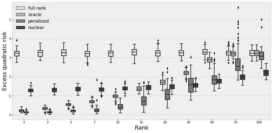 Figure 1
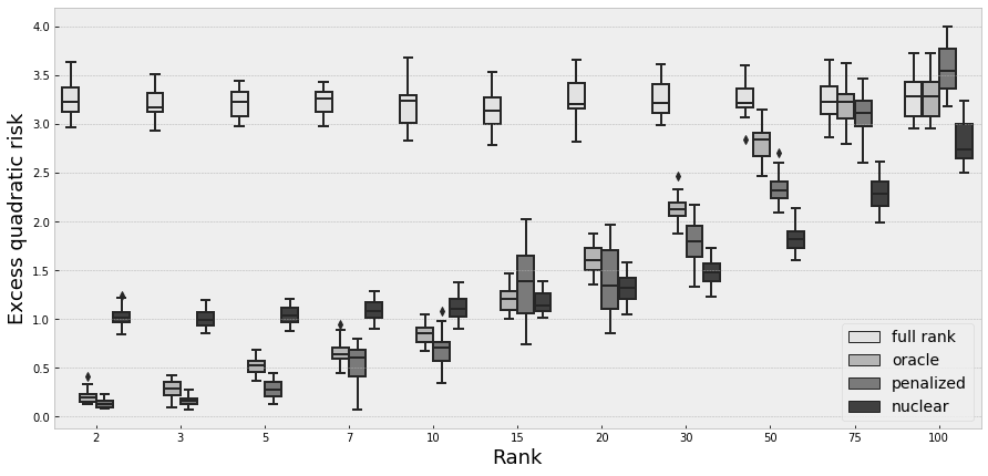 Figure 2
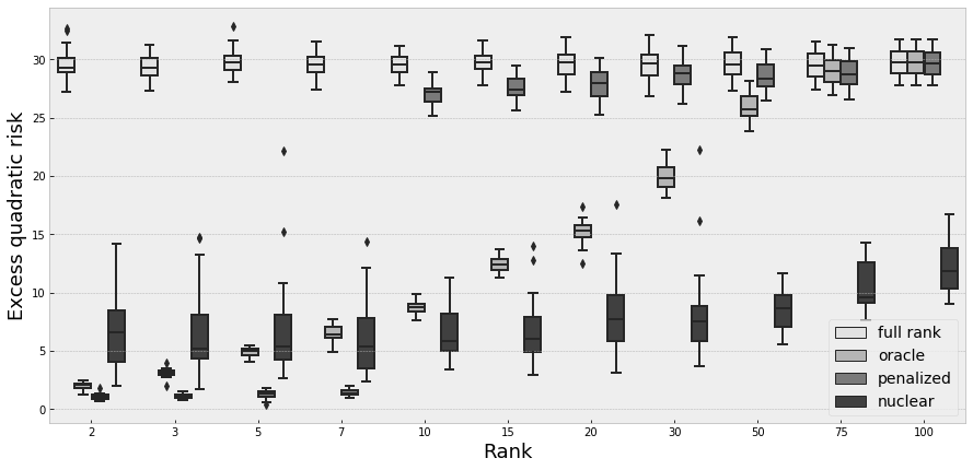 Figure 3
| rank | 2 | 3 | 5 | 7 | 10 | 15 | 20 | 30 | 50 | 75 | 100 | |
|---|---|---|---|---|---|---|---|---|---|---|---|---|
| full rank | 3.27 | 3.21 | 3.21 | 3.23 | 3.20 | 3.15 | 3.27 | 3.26 | 3.25 | 3.24 | 3.28 | |
| nuclear | 1.03 | 1.00 | 1.04 | 1.09 | 1.11 | 1.17 | 1.32 | 1.48 | 1.83 | 2.29 | 2.83 | |
| oracle | 0.21 | 0.28 | 0.51 | 0.66 | 0.85 | 1.21 | 1.60 | 2.13 | 2.81 | 3.19 | 3.28 | |
| penalized | 0.14 | 0.17 | 0.28 | 0.54 | 0.70 | 1.39 | 1.40 | 1.78 | 2.34 | 3.10 | 3.55 | |
| full rank | 3.21 | 3.25 | 3.26 | 3.20 | 3.24 | 3.27 | 3.24 | 3.25 | 3.28 | 3.26 | 3.24 | |
| nuclear | 1.28 | 1.31 | 1.35 | 1.31 | 1.37 | 1.43 | 1.47 | 1.55 | 1.76 | 1.99 | 2.22 | |
| oracle | 0.21 | 0.32 | 0.53 | 0.68 | 0.97 | 1.35 | 1.70 | 2.19 | 2.89 | 3.21 | 3.24 | |
| penalized | 0.12 | 0.13 | 0.20 | 0.25 | 0.41 | 0.74 | 1.07 | 1.57 | 1.89 | 2.78 | 3.10 |
| rank | 2 | 3 | 5 | 7 | 10 | 15 | 20 | 30 | 50 | 75 | 100 | |
|---|---|---|---|---|---|---|---|---|---|---|---|---|
| full rank | 29.59 | 29.34 | 29.91 | 29.54 | 29.59 | 29.74 | 29.62 | 29.52 | 29.67 | 29.49 | 29.68 | |
| nuclear | 6.73 | 6.83 | 6.95 | 6.11 | 6.59 | 6.92 | 8.33 | 8.44 | 8.59 | 10.54 | 12.19 | |
| oracle | 2.00 | 3.09 | 4.88 | 6.52 | 8.75 | 12.41 | 15.22 | 19.90 | 26.03 | 29.03 | 29.68 | |
| penalized | 1.04 | 1.09 | 1.27 | 1.43 | 27.05 | 27.55 | 27.83 | 28.66 | 28.62 | 28.75 | 29.64 | |
| full rank | 7.30 | 7.26 | 7.26 | 7.27 | 7.39 | 7.24 | 7.25 | 7.23 | 7.39 | 7.37 | 7.19 | |
| nuclear | 1.07 | 1.06 | 1.13 | 1.23 | 1.41 | 1.47 | 1.71 | 2.11 | 2.96 | 3.97 | 4.93 | |
| oracle | 0.52 | 0.77 | 1.16 | 1.61 | 2.13 | 2.90 | 3.69 | 4.87 | 6.54 | 7.26 | 7.19 | |
| penalized | 0.29 | 0.31 | 0.44 | 0.71 | 1.12 | 2.19 | 5.77 | 6.74 | 6.85 | 7.05 | 7.33 | |
| full rank | 3.27 | 3.21 | 3.21 | 3.23 | 3.20 | 3.15 | 3.27 | 3.26 | 3.25 | 3.24 | 3.28 | |
| nuclear | 1.03 | 1.00 | 1.04 | 1.09 | 1.11 | 1.17 | 1.32 | 1.48 | 1.83 | 2.29 | 2.83 | |
| oracle | 0.21 | 0.28 | 0.51 | 0.66 | 0.85 | 1.21 | 1.60 | 2.13 | 2.81 | 3.19 | 3.28 | |
| penalized | 0.14 | 0.17 | 0.28 | 0.54 | 0.70 | 1.39 | 1.40 | 1.78 | 2.34 | 3.10 | 3.55 | |
| full rank | 1.53 | 1.52 | 1.52 | 1.57 | 1.50 | 1.57 | 1.49 | 1.52 | 1.52 | 1.57 | 1.53 | |
| nuclear | 0.73 | 0.73 | 0.73 | 0.80 | 0.76 | 0.84 | 0.83 | 0.92 | 1.07 | 1.29 | 1.42 | |
| oracle | 0.08 | 0.12 | 0.20 | 0.30 | 0.38 | 0.56 | 0.69 | 0.95 | 1.29 | 1.54 | 1.53 | |
| penalized | 0.05 | 0.30 | 0.74 | 1.10 | 0.29 | 0.38 | 1.20 | 1.38 | 1.58 | 1.53 | 2.07 | |
| full rank | 0.60 | 0.57 | 0.60 | 0.61 | 0.61 | 0.62 | 0.59 | 0.61 | 0.58 | 0.57 | 0.62 | |
| nuclear | 0.39 | 0.36 | 0.39 | 0.40 | 0.41 | 0.43 | 0.42 | 0.46 | 0.47 | 0.51 | * | |
| oracle | 0.04 | 0.05 | 0.07 | 0.10 | 0.14 | 0.20 | 0.25 | 0.38 | 0.48 | 0.55 | 0.62 | |
| penalized | 0.07 | 0.03 | 0.14 | 0.47 | 0.60 | 0.16 | 0.43 | 1.02 | 1.81 | 1.45 | 1.02 |
| Method | Small | Medium | Large |
|---|---|---|---|
| Constant Trend | 4.72 | 4.72 | 4.72 |
| Independent AR(1) | 4.56 | 4.56 | 4.56 |
| VAR(1) | 3.58 | 2.70 | 2.90 |
| penalized VAR(1) | 3.57 | 2.78 | 2.84 |
| -model | 3.87 | 2.58 | 2.83 |
| Method | Small | Medium | Large |
|---|---|---|---|
| Constant Trend | 1.23 | 1.23 | 1.23 |
| Independent AR(1) | 1.19 | 1.19 | 1.19 |
| VAR(1) | 1.18 | 1.08 | 1.11 |
| penalized VAR(1) | 1.18 | 1.08 | 1.09 |
| -model | 1.17 | 1.10 | 1.15 |
Peer Reviews
No public reviews on file for this paper yet. If you reviewed it on a platform where reviews are public (OpenReview, ICLR, NeurIPS, ICML), you can paste yours below so the community can read it here.
Videos
No videos yet. Explain this paper in a talk, walkthrough, or lecture? Add one.
High dimensional VAR with low rank transition
Pierre Alquier*(1)111This author gratefully acknowledges financial support from the research programme New Challenges for New Data from LCL and GENES, hosted by the Fondation du Risque and from Labex ECODEC (ANR-11-LABEX-0047)., Karine Bertin(2), Paul Doukhan(3,2)222The work of the second and the third author has been developed within the MME-DII center of excellence (ANR-11-LABEX-0023-01) and with the help of PAI-CONICYT MEC N∘ 80170072. The authors have been supported by Fondecyt project 1171335 and Mathamsud 18-MATH-07., Rémy Garnier(4,3)*
*(1) RIKEN, Center for Advanced Intelligence Project, 1-4-1 Nihonbashi Chuo-ku, Tokyo, JAPAN
(2) CIMFAV, Universidad de Valparaíso. General Cruz 222 – Valparaíso, CHILE
(3) Laboratoire AGM UMR 8088, Université Paris Seine, 2 Bd. Adolphe Chauvin, 95000 Cergy-Pontoise, FRANCE
(4) CDiscount, 120 Quai de Bacalan, 33000 Bordeaux, FRANCE *
Abstract
We propose a vector auto-regressive (VAR) model with a low-rank constraint on the transition matrix. This model is well suited to predict high-dimensional series that are highly correlated, or that are driven by a small number of hidden factors. While our model has formal similarities with factor models, its structure is more a way to reduce the dimension in order to improve the predictions, rather than a way to define interpretable factors. We provide an estimator for the transition matrix in a very general setting, and study its performances in terms of prediction and adaptation to the unknown rank. Our method obtains good result on simulated data, in particular when the rank of the underlying process is small. On macro-economic data from Giannone et al., (2015), our method is competitive with state-of-the-art methods in small dimension, and even improves on them in high dimension.
1 Introduction
Machine learning became omnipresent in time series forecasting. With the growing ability to collect and store data, one often has to predict series with dimensions from a few hundreds (for economic time series see Jochmann et al., (2013)) to millions (as it might be the case for sales forecasts for a huge set of items, see for example Kumar and Patel, (2010)). The applications fields range from health data analysis (Lipton et al., (2016)), electricity consumption forecasting (Gaillard et al., (2016); De Castro et al., (2017)), economics and GDP forecasting (Cornec, (2014)), traffic forecasting (Lippi et al., (2013)) and public transport attendance (Chapter 5 in Carel, (2019)), social media analysis (Saha and Sindhwani, (2012)), ecology (Purser et al., (2009)), sensor data analysis (Basu and Meckesheimer, (2007))… In many of these applications, accurate predictions are of the uttermost importance. For online retail, a bad prediction of the sales before Christmas might lead to inadequate storage and huge losses of money. Poor electricity forecasts might lead to power outage. When it comes to health data, a good prognosis may even be vital…
In many cases, algorithms that were primarily designed for i.i.d. observations are used on time series with good results. For example, the additive model of Buja et al., (1989) is used in Carel, (2019) to predict bus lines attendance, with promising results. While generalization bounds were developed first for i.i.d data (see e.g Vapnik, (1998) for an overview), some authors actually proved similar results when the same algorithms are applied on time series. We refer the reader to the pioneering work of Meir, (2000) and Steinwart with various co-authors (see Steinwart and Christmann, (2009); Steinwart et al., (2009); Hang and Steinwart, (2014) for an early overview). Model selection tools are investigated in Alquier and Wintenberger, (2012); McDonald et al., (2017) while aggregation methods are studied via PAC-Bayesian bounds in Alquier and Li, (2012); Alquier et al., (2013); Shalizi and Kontorovich, (2013); London et al., (2014); Alquier and Guedj, (2018). While these results hold for stationary series, some authors also tackled non-stationary series. De-trending techniques are considered in Chen and Wu, (2018) while Kuznetsov and Mohri, (2015); Alquier et al., 2019b directly prove generalization bounds on non-stationary series. An original approach was also developed in Giraud et al., (2015) for time-varying AR, relying on sequential prediction methods (Cesa-Bianchi and Lugosi, (2006)).
However, we believe that there is a need to develop machine learning methods that aim at capture stylized facts in time series, in the same spirit that stochastic volatility models were developed to capture stylized facts in finance (see Engle, (1995); Francq and Zakoian, (2019)). In this paper, we study a vector auto-regressive (VAR) that is suitable to predict high-dimensional series that are strongly correlated, or that are driven by a reasonable number of hidden factors, in the spirit of factor models studied in econometrics Koop and Potter, (2004); Lam et al., (2011); Giordani et al., (2011); Lam and Yao, (2012); Hallin and Lippi, (2013); Chan et al., (2018). It is to be noted that factor models naturally lead to low-rank transition matrices. However, in our case, the focus is not on the interpretation of these factors, but on the prediction of the time series. Indeed, even though the series is not driven by a small number of hidden factors, the low-rank constraint on the transition matrix induces a dimension reduction that can improve the predictions, as in Negahban and Wainwright, (2011); see also Basu et al., (2019) who used such a constraint to detect outliers. We believe that this constraint makes often more sense than sparsity constraints used for example in Davis et al., (2016). On the contrary to Negahban and Wainwright, (2011), we focus on the prediction ability of our estimator. We study its prediction performances under a general loss function. While the quadratic loss or the absolute loss are indeed useful, quantile losses can also be used to derive confidence intervals.
Let us briefly describe the motivation for our models. Assume we deal with an -valued process with
[TABLE]
for a very large . First, in the hidden factor model, it is assumed that factors , that are linear functions of , drive the evolution of the process (as a simple example, can be the GDP of each country, and the hidden factors can reflect the general state of the economics at a continent scale). We can write them as where is with . Then, assuming that can be linearly predicted by , we can predict by for some matrix . At the end of the day, we indeed predict by , but the rank of is . However, note that even in situations where we cannot clearly identify hidden factors, a low-rank assumption makes sense. For example, if all the series in are strongly correlated, then can be reasonably well approximated by a rank-one matrix. Hence, to impose a low-rank constraint on the transition matrix (here we assume that the matrix has a rank ) will highly reduce the variance, at the price of a small increase of the bias term. This might lead to improved predictions.
Note that the assumption that the coefficient matrix is low-rank in a multivariate regression model where and was studied in Econometric theory as early as in the 50’s (Anderson, (1951); Izenman, (1975)). It was referred to as RRR (reduced-rank regression). We refer the reader to Koltchinskii et al., (2011); Bunea et al., (2011); Suzuki, (2015); Alquier et al., 2019a ; Klopp et al., (2017); Bing and Wegkamp, (2019); Klopp et al., (2019); Moridomi et al., (2018) for state-of-the-art results. Low-rank matrices were actually used to model high-dimensional time series by De Castro et al., (2017) and Alquier and Marie, (2019), however, the models described in these papers cannot be straightforwardly used for prediction purposes. Here, we study estimation and prediction for the model (1).
More precisely, we propose two estimators of the matrix : a fixed-rank estimator and a rank-penalized estimator. The first one is obtained minimizing an empirical prediction error based on a Lipschitz loss function among a specific family of matrix with given rank . In the second one, a procedure based on rank penalization of our empirical error allows us to select a rank and we finally consider the fixed-rank estimator with rank . As we mentioned before, we study properties of both estimators in terms of prediction. We prove that the rank-penalized estimator satisfies an oracle inequality adapting to unknown rank. We illustrate performances of our estimators on simulated data and a macro-economic dataset from Giannone et al., (2015). We also compare our estimators to near low-rank or nuclear estimators proposed in Negahban and Wainwright, (2011) and Ji and Ye, (2009).
The paper is designed as follows. In the end of the introduction, we provide notations that will be used in the whole paper. We describe our low rank contractive VAR(1) model in Section 2; contraction yields the existence of a stationary solution and together yields standard weak dependence properties. The two estimators and their properties are given in Section 3 whereas the simulation study and application to real data set are presented in Sections 4 and 5. Finally, the proofs of the results of Section 3 are postponed to Section 7.
Notations
We introduce here notations that are used in the whole paper. For a vector , will denote the Euclidean norm of . We will denote by the singular values of an matrix , where . Note that the singular value decomposition (SVD) of can be written
[TABLE]
for some semi-unitary matrices and : , where is the identity matrix. This means that, from the implicit function theorem, the set of such matrices is a subspace of a Riemanniann manifold with dimension .
For we let denote the Schatten--norm of defined by
[TABLE]
if , and . For and , we define:
[TABLE]
2 Vector auto-regressive process with low-rank constraint
We consider the -valued VAR process , defined from (1), where are i.i.d and centered random variables and where the matrix satisfies assumption:
Assumption 1**.**
We assume that for some and .
For now, the rank assumption is not restrictive, as the largest possible value is not forbidden. However, we will see that a smaller will lead to better rates of convergence in terms of prediction.
The assumption is more restrictive, but it is important in what follows. Indeed, setting , the following contraction property holds:
[TABLE]
which yields in case of the existence of a moment for , . This implies the -dependence property (with a geometric decay, ) and the ergodicity of this model (see Dedecker et al., (2007)). The assumption also implies that the matrix is invertible and its inverse writes as
[TABLE]
The stationary distribution of this model is the distribution of . From now, we will assume that , that is, the process is stationary. In the special case of Gaussian noise then
[TABLE]
We also introduce the following assumption.
Assumption 2**.**
There exist some positive constants and such that the noise process satisfies for all
[TABLE]
This assumption is for example satisfied for a Gaussian noise , but it also holds in any case where the components of are independent and follow any sub-Gaussian distribution, such as a bounded distribution. Assumption 2 is not required for the process to be well defined. However, we will use it to derive our theoretical results on estimation and prediction.
3 Estimators, prediction and rank selection
Following the approach described in Vapnik, (1998), we measure the quality of an estimator by its generalization ability, that is, by its out of sample prediction performances. The quality of a prediction will be assessed by a loss function : stands for the cost of having predicted when the truth appears to be .
Assumption 3**.**
The loss function is -Lipschitz with respect to the Euclidean norm for some . That is, for all , .
We impose the condition for the sake of simplicity, but note that it is not restrictive as we can rescale the loss anyway. This includes, for example, the Euclidean norm or the max norm . However, the squared Euclidean norm, , only satisfies Assumption 3 when the process and the predictions are bounded.
We are now in position to define the generalization error.
Definition 3.1**.**
The generalization error of an matrix is given by
[TABLE]
Note that does not depend on as is stationary. Given a sample we can obviously estimate this error by its empirical counterpart, and define an estimator based on empirical risk minimization.
Definition 3.2** (Fixed-rank estimator).**
The empirical error of an matrix is given by
[TABLE]
The rank empirical risk minimizer (or fixed-rank estimator), , is defined, for any , by
[TABLE]
Note that in Assumption 3, we only required the loss to be Lipschitz. However, in practice, loss functions that are also convex will be preferred in order to ensure the feasibility of the minimization of the empirical risk.
Remark 3.1*.*
Algorithms are known to compute such a low-rank factorization in practice. The most popular method is to write for matrices and , and to optimize with respect to and (the constraint can be ensured for example by imposing and ). The popular ADMM method boils down to the alternate minimization with respect to and , see Section 9 in Boyd et al., (2011). This strategy works well in practice, despite its lack of theoretical support in this situation. Even when is convex, the minimization problem is usually non convex with respect to the pair . Still, recent works Ge et al., (2017) shows that this non-convexity is not “severe” in the sense that it is still possible to find a global minimum in a reasonable time. When is not convex, it is not currently known how to compute the exact minimizer in a feasible time.
The following condition is purely technical and will only be used to make more accurate the statement “for large enough”.
Assumption 4**.**
We have where and .
Theorem 3.1**.**
Let Assumptions 1, 2, 3 and 4 hold. Then for any , with probability larger than , we have
[TABLE]
Corollary 3.2**.**
Let Assumptions 1, 2, 3 and 4 hold. For any fixed , we have with probability larger than
[TABLE]
where denotes a positive constant, only depending on , , and .
Corollary 3.3**.**
Let Assumptions 1, 2, 3 and 4 hold. For , we have for some suitable positive constant depending on , and that
[TABLE]
with probability larger that .
Remark 3.2*.*
[Variations on low rank VAR(1)] Instead of considering finite rank matrices, an alternative is to consider a low rank perturbation around another matrix. As an example, the -model consists in a diagonal matrix , and . Then is estimated as in the so-called AR case with decoupled (independent) AR(1)-models in one dimension. The parameter set is now a subset of a Riemanniann manifold with dimension . Recall that, in order that be estimable, the AR(1)-coordinate models must be stable thus their coefficients belong . Indeed and imply with rank that .
Coming back to the low rank model, note that if the true rank of is known, then leads to
[TABLE]
which means that the estimator predicts as well as the true matrix when and , satisfy . This is true when and are constants, but also covers high-dimensional asymptotics like and . However, this estimator requires the knowledge of , which is usually not the case. For this reason, we now describe a model selection procedure for , based on rank penalization.
Definition 3.3** (Rank-penalized estimator).**
Let Assumption 4 holds for at least one value . Define as the largest integer such that . The rank-penalized estimator is defined by where
[TABLE]
In practice, in order to compute , we need to know , and which is still not realistic. However, for such a model selection by penalized risk minimization, it is known anyway that the constants in front of the penalization are usually too large. The slope heuristic leads to better results in practice Birgé and Massart, (2007); Baudry et al., (2012), we provide more details in Section 4. We now provide a theoretical study of the rank-penalized estimator. The following theorem states this estimator predicts almost as well as the best fixed-rank estimator. Of course, which fixed-rank estimator is the best is not known in advance, hence, this estimator is often referred to as the oracle, and the inequality in the theorem as an oracle inequality.
Theorem 3.4**.**
Let Assumptions 1, 2, 3 and 4 hold. Let . With probability at least , we have
[TABLE]
A more precise analysis of the involved factors yields the following corollaries.
Corollary 3.5**.**
Under Assumptions 1, 2, 3 and 4, for any fixed ,with probability larger than
[TABLE]
where and are positive constants depending on , , and .
Corollary 3.6**.**
Let Assumptions 1, 2, , 3 and 4 hold. For , we have for some suitable positive constant depending on , and that
[TABLE]
with probability larger that .
When is large enough so that , we obtain
[TABLE]
so the estimator is adaptive: it does not depend on .
4 Simulations
4.1 Simulation design
In order to evaluate the performance of low-rank reconstruction, we run simulations for different values of the parameters and . We set to have reasonable computation time. The simulations are done with Python and are available online (Garnier, (2019)).
More precisely, for fixed,
- •
we generate a matrix of rank , as in (2), by setting
[TABLE]
where and are semi-unitary matrices and is a diagonal matrix whose diagonal coordinates follow a distribution Beta of parameters and . The matrices and are obtained making orthogonal two matrices whose coefficients are i.i.d uniform on . Therefore, when , the distribution of the singular values of is uniform. When is smaller, the singular values tend to be smaller and is close to some matrix with lower rank.
- •
we generate a sample of length from an valued VAR(1) process with
[TABLE]
where the are truncated centered Gaussian variables with variance , where the i.i.d. coordinates admit the support , and .
For each triplet , such a data set is simulated times.
4.2 Estimators and quality criteria
Our estimation procedures use the quadratic loss, that is
[TABLE]
where we denote by the Euclidean norm on . The use of quadratic loss allows one to obtain exact expression for some of the minimization, which speeds up convergence. Note also that since we use truncated Gaussian Noise, Assumption 3 is satisfied.
We compare several estimators in which minimization of this empirical risk (penalized or not) over has to be computed. We use in the simulations . As we state in Remark 3.1, we look for minimizers of the form for matrices and , and we optimize with respect to and by imposing and ). We use here the ADMM method that alternates minimization with respect to and .
For each simulation, we compute four estimators:
- •
The standard full-rank VAR(1) estimator magenta(the fixed-rank estimator with rank ) for the quadratic loss, i.e.:
[TABLE]
- •
The oracle VAR(1) (the fixed rank estimator with rank ), where we suppose that we know the underlying rank .
[TABLE]
- •
The rank-penalized estimator. Note that this estimator can also be rewritten as
[TABLE]
where depend on , and several unknown constants given in Definition 3.3. We choose to implement a simpler (and not so different) version of this estimator given by
[TABLE]
This second estimator have similar performances to (5) for small rank and performs better for higher ranks. As we explained in Section 3 the constant in the penalty of the rank-penalized estimator is however too large in practice. A very popular way to fix this is to calibrate this constant via the slope heuristic. This is what we do here. The slope heuristic can be summarized as follows. One studies how decreases when grows. Select as an estimator where corresponds to the largest decay in . The slope heuristic was introduced by Birgé and Massart, (2007), more details on its implementation are given in Baudry et al., (2012) and its theoretical optimality (for i.i.d data) is studied in Arlot and Massart, (2009). We refer the reader to Arlot, (2019) for a recent overview.
- •
The near low-rank estimator that we called here nuclear as defined in Negahban and Wainwright, (2011) or Ji and Ye, (2009). It introduces an empirical risk minimization penalized by the nuclear norm . We use the method proposed in Ji and Ye, (2009) to compute an approximation of this solution. We also use the slope heuristics to compute the penalization constant
[TABLE]
We want to study the performances of our estimators and to compare them with usual nuclear estimator. As we are interested in studying performances in terms of prediction, to assess the quality of an estimator , we calculate the excess risk computed on a new sample generated as in the previous part with the same matrix used to generate our data:
[TABLE]
where
[TABLE]
4.3 Results
We perform simulations for different values for the triplets . The results are given in the following tables and figures. Tables 1 and 2 contain the mean of the excess risk over the simulations for the four estimators and different values of , , and . Figures 1 to 3 show the dispersion of the excess risk over the simulations for and and for and
Moreover means that the convergence step of the algorithm was too important.
General Remarks
Performing a full-rank estimation of a matrix of low rank is generally the worst solution. It is normal, because the overfitting is much more important in this case. It doesn’t exploit the underlying small rank aspect, so the performance doesn’t change with .
For all other estimator, the performance degrades with . In particular for both penalized and nuclear estimator, it is possible to have worst performance than the full-rank estimator when the underlying rank is closed to M, in particular when the dispersion of singular values is uniform () . It is also logical, as in this case we are far from the low rank setting, and the penalization becomes a drawback. When , oracle and full rank estimators are the same.
We also remark that the excess risk decreases when increases. When we are really close to the high-dimensional case (), a rank threshold appears in the performance of the penalized estimator. Below this rank, the penalized estimator have a good performance. Above this threshold, the penalized estimator has the same performance than the full rank estimator. It suggests that, in this case, the rank chosen by the penalized estimator is close to .
Comparison with oracle estimator
When the rank is small, our penalized estimator outperforms the oracle estimator. It is especially the case when we have few observations. In fact, in this case, the penalized estimator choose generally a smaller rank than , and it has then less parameters to fit, avoiding generally overfitting. However, this effects becomes a drawback when or increases: then, the complexity of the estimation grows, and therefore the estimation error. When the number of small singular values is important (), the penalized estimator improves its performance, as the model behaves like a small-rank.
Comparison with nuclear estimator
Generally the performances of the nuclear estimator are less-rank sensitive than the performance of oracle or penalized estimator. Our hypothesis is that nuclear estimator only performs near low-rank approximation, and that it is harder to be near a "good" very small rank matrix than a "good" larger one. This implies that our models outperforms nuclear estimator in small rank settings (or when ), but it is outperformed when the rank is higher. The penalized estimator has, relatively, a better performance when is small.
5 Application to a macro-economic data-set
We want to evaluate the performances of our estimations on real-world datasets. We use macro-economical data known used in Giannone et al., (2015). It consists in different US economic indicator. We used the three different datasets:
- •
A small dataset containing quarterly times series between 1959 and 2008.
- •
A medium dataset containing quarterly times series between 1959 and 2008.
- •
A large dataset containing quarterly times series between 1959 and 2006.
The datasets are described with more details in Giannone et al., (2015). We weren’t able to get those whole datasets; hence our results are not easy to compare with those of Giannone et al., (2015).
In order to test the models, we estimate them by using the data between 1959 and 2001, and perform prediction on the period 2001-2006 for GDP (Gross domestic product) and GDP deflator (also called implicit GDP, this is a measure of the level of prices of all new, domestically produced, final goods and services in an economy in a year). We evaluate this prediction using the Mean Squared Error (MSE).
We compare the performances of 5 predictors.
- •
First, we use a naive predictor which asserts a constant trend at each date.
- •
The second prediction is obtained assuming independent AR(1)-models for each series.
- •
In the third, we use the full rank estimator.
- •
The fourth predictor is the one based on our rank-penalized estimator.
- •
In the fifth predictor, we consider the -model introduced in the Remark 3.2.
We sum up the results in Tables 3 and 4. The penalized VAR estimator has better results than the Naive or Independent AR estimator on all the datasets. The full-rank VAR algorithm outperforms it for the small or medium datasets. However, if we increase the number of features (or series), the performance of the penalized VAR is less affected than the performance of the full-rank VAR estimator. We suggest that it performs a form of features selection, which reduces over-fitting.
The -model outperforms all other models on GDP forecasts, but the VAR models are better on GDP deflators forecasts. It suggests that the low rank hypothesis may be adapted in other contexts than pure VAR(1) regression.
6 Conclusion
We considered a rank-constrained VAR model to predict high-dimensional time series. We proposed a theoretical study of our estimator and proved that it leads to consistent predictions. However, many questions remain opened. Faster rates should be possible for strongly convex losses, in the spirit of Alquier et al., (2013). It would also be necessary to study the performances of the slope heuristic from a theoretical point of view, as was done in the i.i.d setting by Arlot and Massart, (2009); Arlot, (2019).
The properties of the -models introduced in Remark 3.2 are checked in § 5; the use of such models deserves a special attention. Finally other heteroskedastic models may be investigated. E.g.:
- •
(V)ARCH models may be rewritten from a more elementary rewriting of Bauwens et al., (2006)
[TABLE]
for some symmetric positive matrix valued quadratic form. Recall that the non negative square root of a positive definite matrix exists and is indeed unique. A simple example of this situation is a diagonal quadratic form
[TABLE]
with for non-negative -matrices . Poignard, (2019) introduces analogous models with sparsity considerations instead of our suggested of a rank restriction. The rank condition turns as the fact that all the matrices admit a same decomposition (2) wrt rank
[TABLE]
- •
(V)INARCH models
[TABLE]
for defined by i.i.d. arrays of Poisson processes, some , and some -matrix with non-negative coefficients. The low rank model writes here with ;
- •
(V)INAR models (defined through thinning operators)
[TABLE]
for some -matrix with non-negative coefficients, here stands for the thinning operator. The low rank model writes again with .
More examples could be inspired from the models detailed in Doukhan, (2018). One may think of multiple Volterra processes, bilinear models, switching VAR models, etc…The heteroskedasticity of these models will require new techniques. Indeed, in the proof section below, it will be clear that our results rely on a Bernstein inequality proven in Dedecker and Fan, (2015) that cannot be used for (V)ARCH models. New concentration tools as, for example, those developed in Dedecker et al., (2019) will be used in forthcoming works invoking adapted datasets.
The simulations and the real data study demonstrate that such low rank VAR models are meaningful, in particular when the underlying rank of the process is small. Anyway additional features such as heteroskedasticity need to be taken into consideration. Hence, as this was stressed in the introduction, we believe that there is a urgent need for more models involving low rank assumptions for high-dimensional time series.
7 Proofs
7.1 Preliminaries
Let us start with a few additional notations.
Definition 7.1**.**
When Assumption 2 is satisfied, we put
[TABLE]
where and and where and are the constants defined in Assumption 2.
Note that
[TABLE]
where and , and and are as in Section 3 above.
In Alquier et al., 2019b the authors propose to use an exponential inequality to control the deviations between the generalization error and the empirical risk in the case of a non-stationary Markov chain. We follow the same approach here. The version of Bernstein inequality from Dedecker and Fan, (2015) gives directly the following result.
Corollary 7.1**.**
Under Assumptions 1 and 2 we have, for any matrix ,
[TABLE]
, with .
Proof of Corollary 7.1.
This corollary is a consequence of the Bernstein inequality in Dedecker and Fan, (2015) which requires the following assumption.
Assumption 5**.**
There exist some constants , and such that
[TABLE]
where and are defined by
[TABLE]
Note that for .
[TABLE]
Assumption 2 implies that , for each . With the Euclidean norm thus from Hölder inequality we obtain with
[TABLE]
Consider now some odd number such that then
[TABLE]
since from Stirling inequality and thus ; we also use the relation .
Note that the independence of coordinates is not required.
Since , Assumption 5 is satisfied with
[TABLE]
Moreover has be chosen as an upper-bound of . Then we choose ∎
7.2 Proof of the theorems of Section 3
Proof of Theorem 3.1.
A first issue is to derive some general useful features from empirical processes techniques. Recall that the Frobenius norm of a matrix is satisfies
[TABLE]
Define for of a set of matrices , its covering number with respect to the Frobenius norm.
In their Lemma 3.1, Candès and Plan, (2011) prove a main combinatorial property about the sphere , which is the set of matrices with rank and with Frobenius norm : for , may be covered by an net (in metric) with cardinal
[TABLE]
Now denote and respectively the sphere and the ball of such matrices with rank and with either or .
An homogeneity argument first allows to derive the existence of an net of with cardinal .
Now for , then an net of is provided by with . Then
[TABLE]
Still using we can simplify further inequalities: so . As in addition , one has , which leads to
[TABLE]
The above inequalities relating the various norms imply that and so
[TABLE]
as soon as .
Note that the above covering numbers are considered wrt the Frobenius norm, thus the above inequality also concerns the covering numbers wrt .
Remark 7.1*.*
For the model of Remark 3.2 quote that the bound in (8) admits a right hand side inequality transformed as
[TABLE]
which does not change the structure of the excess risk behaviour.
Fix and (their value will be given later). By using both Corollary 7.1 and the inequality (8), we have
[TABLE]
Now, for any define by
[TABLE]
Obviously
[TABLE]
and as a consequence,
[TABLE]
and
[TABLE]
Applying Bernstein Inequality (3.3) in Proposition 3.1 of Dedecker and Fan, (2015) with and we have, for any ,
[TABLE]
Now let us consider the “favorable” event
[TABLE]
The previous inequalities show that
[TABLE]
On , we have:
[TABLE]
In particular, the choice ensures:
[TABLE]
Note that this choice is allowed: indeed, the only condition on is and . Remind that
[TABLE]
Fix and put:
[TABLE]
and
[TABLE]
Note that, plugged into (9), these choices ensure .
Put
[TABLE]
As soon as , that is actually ensured by the condition , we have:
[TABLE]
Plugging the expressions of and into (10) gives:
[TABLE]
which ends the proof taking into account that and . ∎
Proof of Theorem 3.4.
For short, put
[TABLE]
so that
[TABLE]
For short, put . We keep the notations of the previous proof, we will just change the values of . From the classical union bound argument we derive:
[TABLE]
We take , as in the previous proof and
[TABLE]
which implies
[TABLE]
This leads to
[TABLE]
Also note that for any ,
[TABLE]
Now, on the favorable event we have
[TABLE]
Replace and by their value to obtain
[TABLE]
This ends the proof. ∎
The reference list from the paper itself. Each links out to its DOI / PubMed record.
- 1(1) Alquier, P., Cottet, V., and Lecué, G. (2019 a). Estimation bounds and sharp oracle inequalities of regularized procedures with lipschitz loss functions. The Annals of Statistics , 47(4):2117–2144.
- 2(2) Alquier, P., Doukhan, P., and Fan, X. (2019 b). Exponential inequalities for nonstationary Markov chains. Dependence Modeling , (7):150–168.
- 3Alquier and Guedj, (2018) Alquier, P. and Guedj, B. (2018). Simpler PAC-Bayesian bounds for hostile data. Machine Learning , 107(5):887–902.
- 4Alquier and Li, (2012) Alquier, P. and Li, X. (2012). Prediction of quantiles by statistical learning and application to gdp forecasting. In International Conference on Discovery Science , pages 22–36. Springer.
- 5Alquier et al., (2013) Alquier, P., Li, X., and Wintenberger, O. (2013). Prediction of time series by statistical learning: general losses and fast rates. Dependence Modeling , 1:65–93.
- 6Alquier and Marie, (2019) Alquier, P. and Marie, N. (2019). Matrix factorization for multivariate time series analysis. Electronic journal of statistics , 13(2):4346–4366.
- 7Alquier and Wintenberger, (2012) Alquier, P. and Wintenberger, O. (2012). Model selection for weakly dependent time series forecasting. Bernoulli , 18(3):883–913.
- 8Anderson, (1951) Anderson, T. W. (1951). Estimating linear restrictions on regression coefficients for multivariate normal distributions. The Annals of Mathematical Statistics , 22(3):327–351.