Control Variates for Stochastic Simulation of Chemical Reaction Networks
Michael Backenk\"ohler, Luca Bortolussi, Verena Wolf

TL;DR
This paper introduces a variance reduction method using control variates for stochastic simulations of chemical reaction networks, significantly decreasing the number of runs needed for accurate estimations.
Contribution
It presents a novel on-line algorithm for selecting control variates based on moment constraints, improving computational efficiency in stochastic chemical modeling.
Findings
Reduced variance in estimators across case studies
Fewer simulation runs required for accurate results
Demonstrated efficiency of the control variate approach
Abstract
Stochastic simulation is a widely used method for estimating quantities in models of chemical reaction networks where uncertainty plays a crucial role. However, reducing the statistical uncertainty of the corresponding estimators requires the generation of a large number of simulation runs, which is computationally expensive. To reduce the number of necessary runs, we propose a variance reduction technique based on control variates. We exploit constraints on the statistical moments of the stochastic process to reduce the estimators' variances. We develop an algorithm that selects appropriate control variates in an on-line fashion and demonstrate the efficiency of our approach on several case studies.
Click any figure to enlarge with its caption.
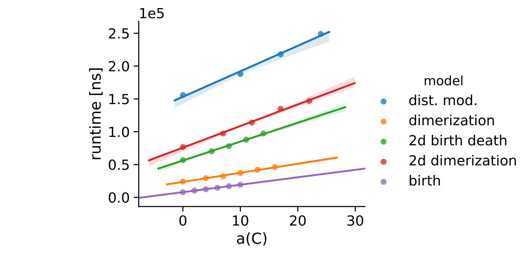 Figure 1
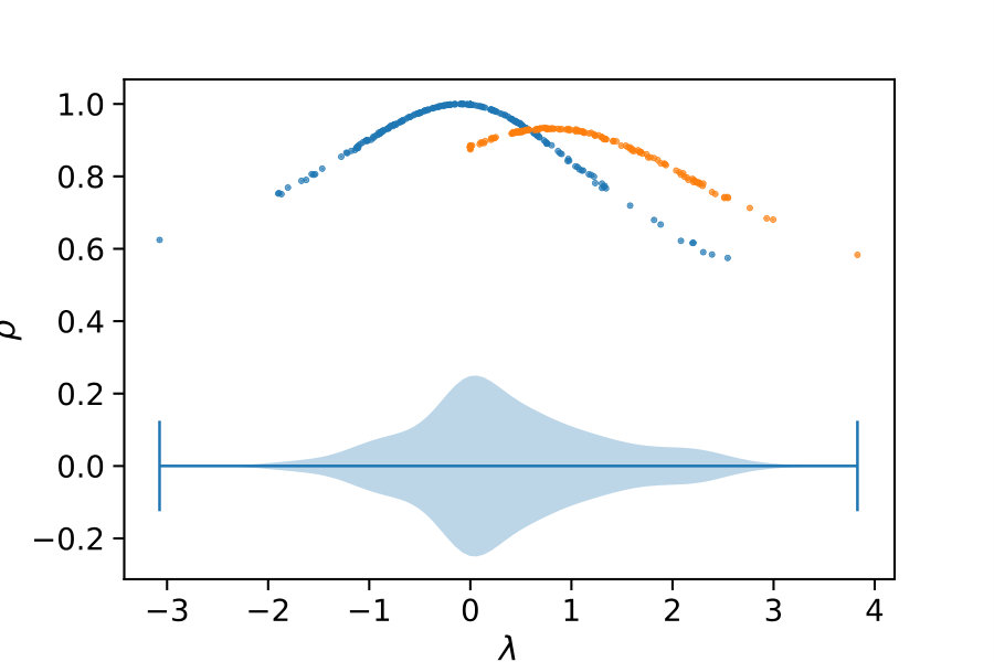 Figure 2
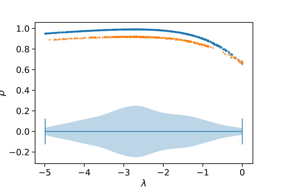 Figure 3
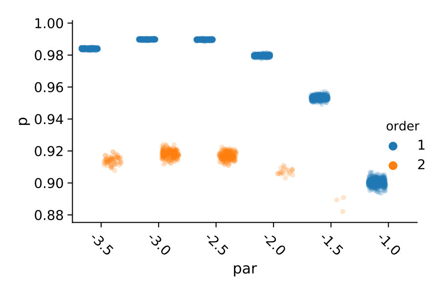 Figure 4
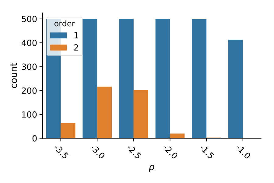 Figure 5
 Figure 6
 Figure 7
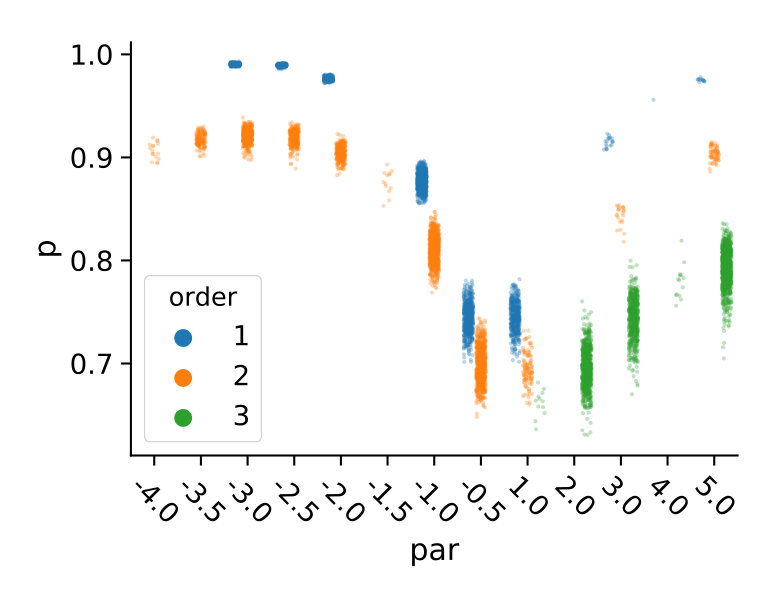 Figure 8
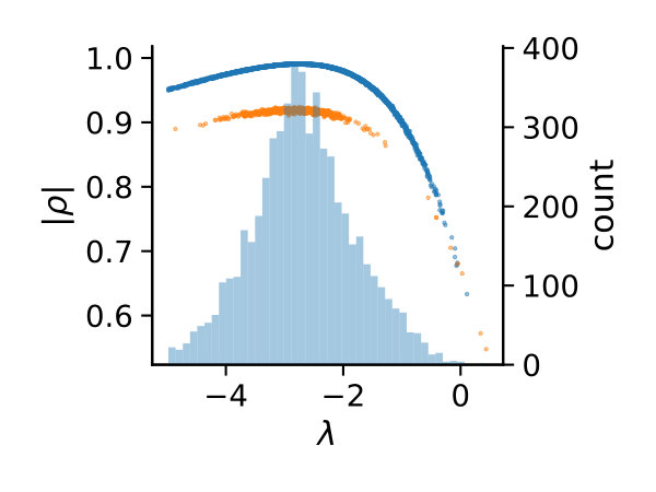 Figure 9
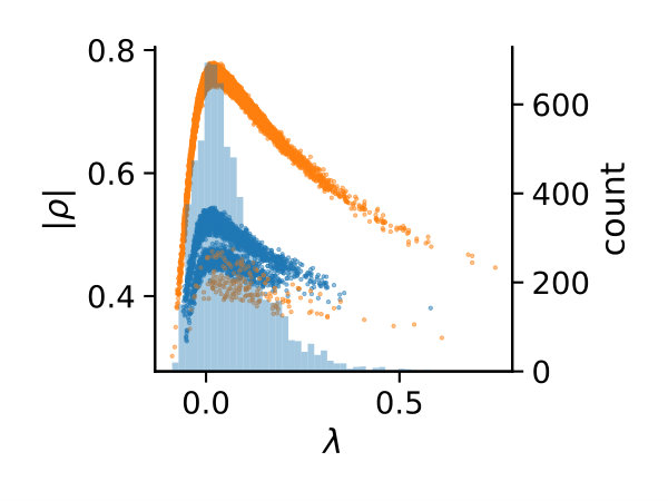 Figure 10
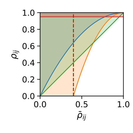 Figure 11
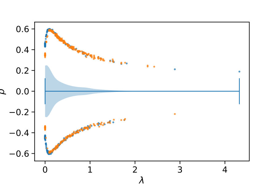 Figure 12
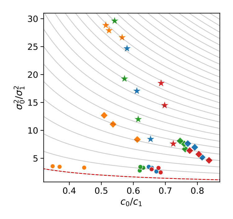 Figure 13
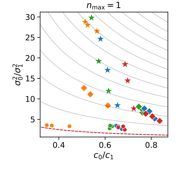 Figure 14
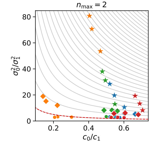 Figure 15
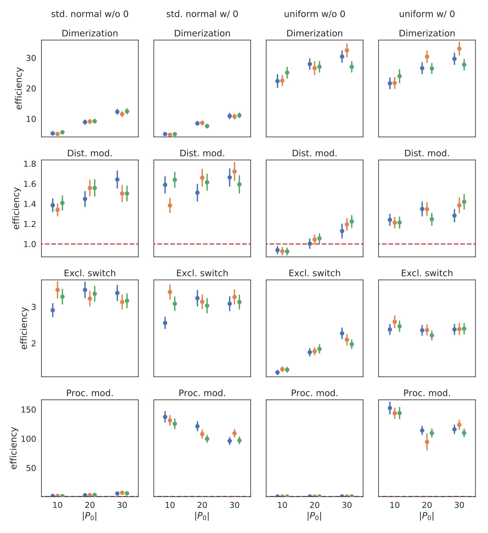 Figure 16
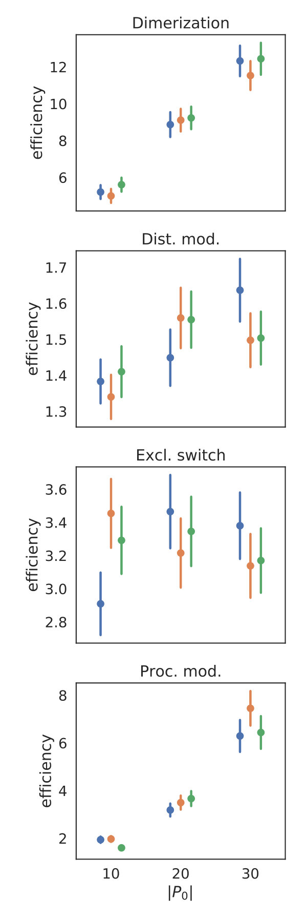 Figure 17
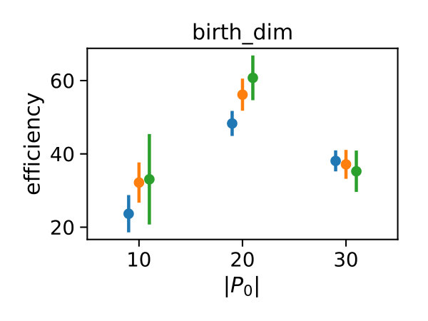 Figure 18
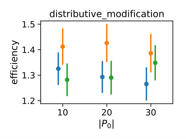 Figure 19
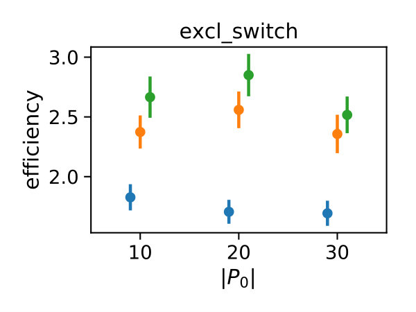 Figure 20
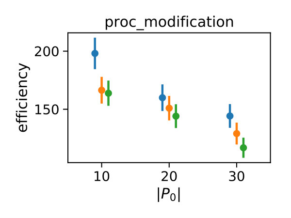 Figure 21
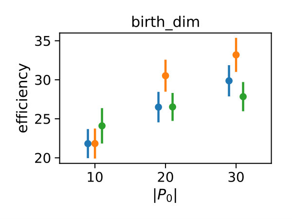 Figure 22
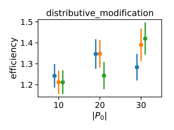 Figure 23
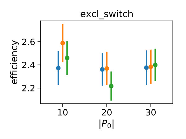 Figure 24
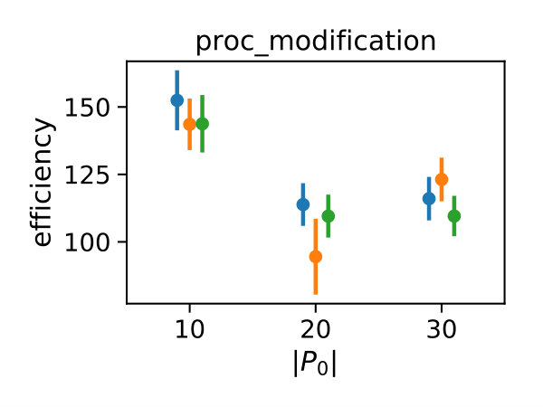 Figure 25
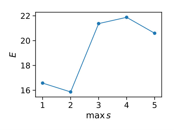 Figure 26
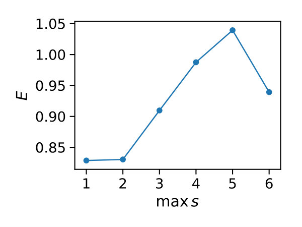 Figure 27
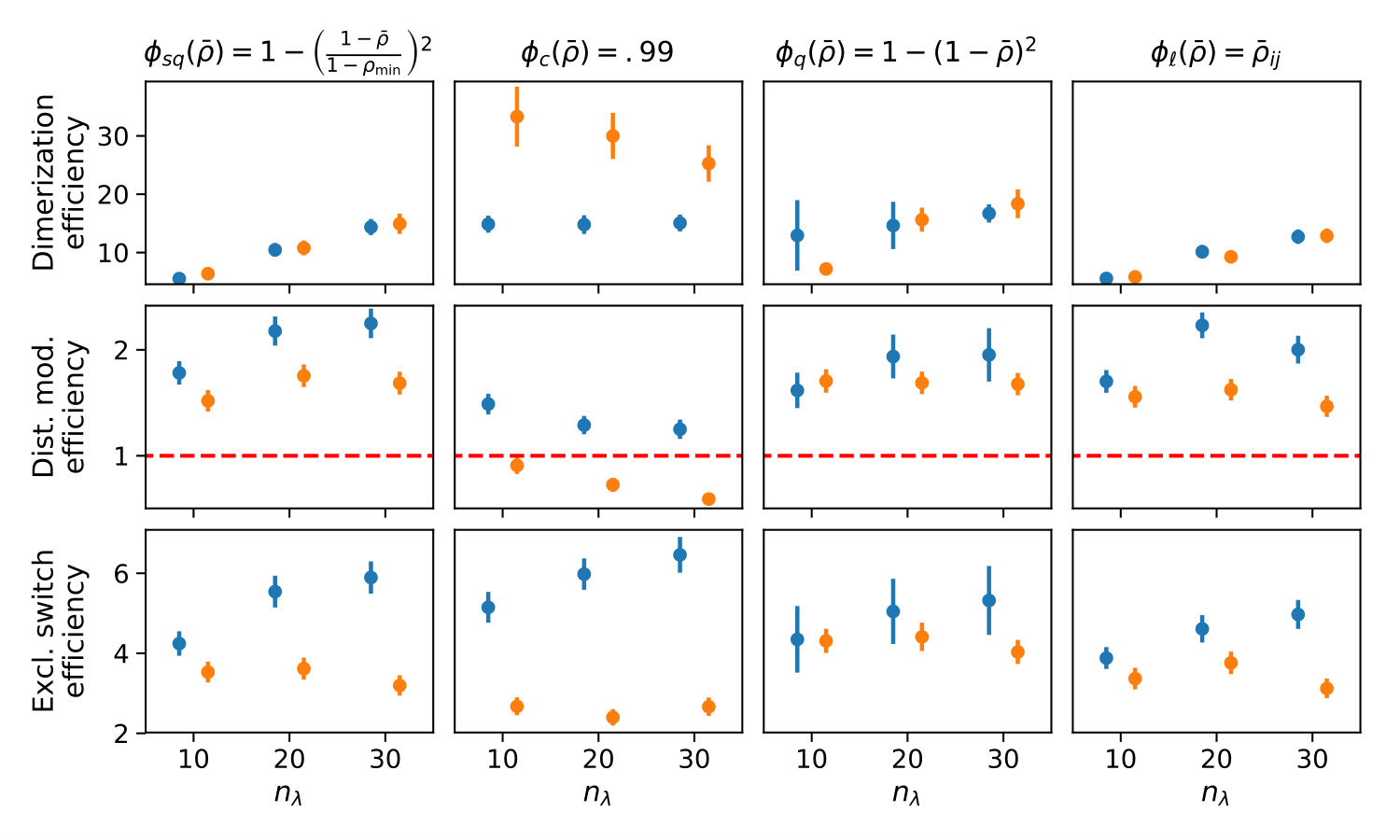 Figure 28
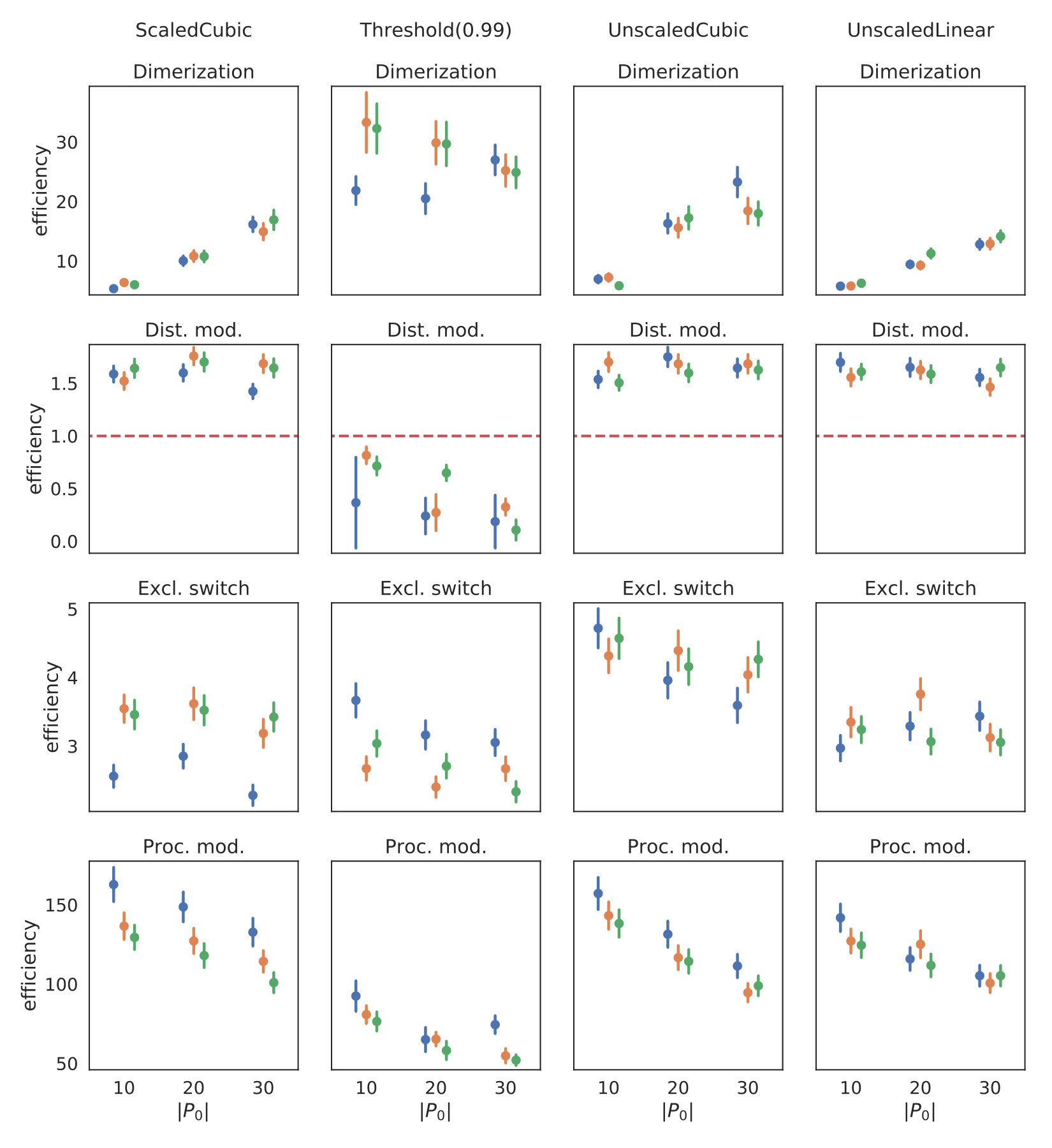 Figure 29
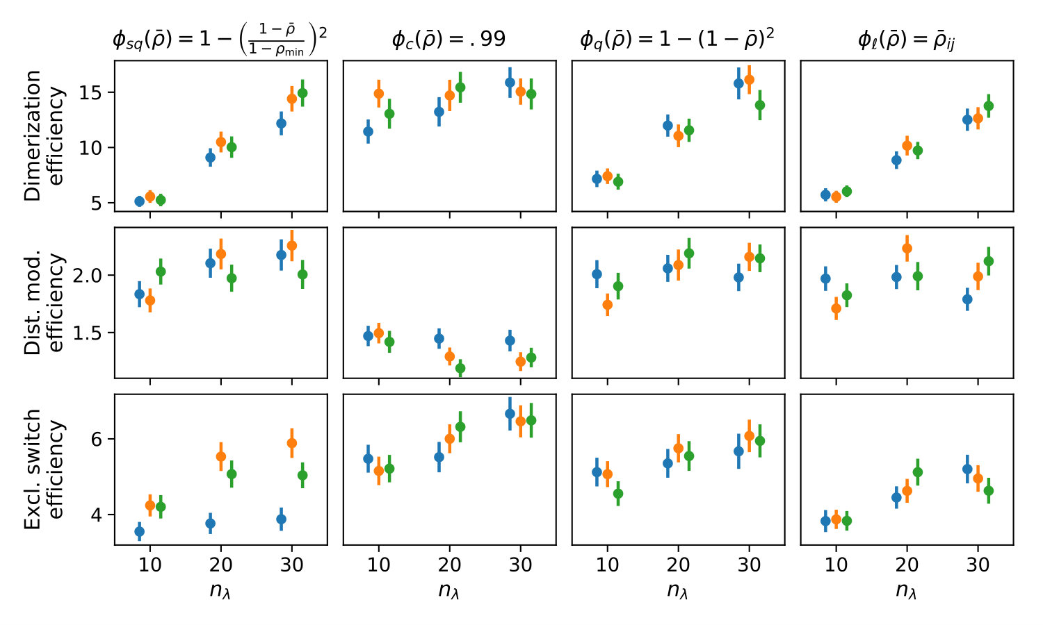 Figure 30
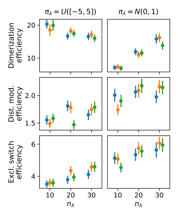 Figure 31
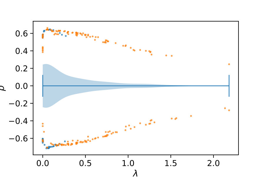 Figure 32
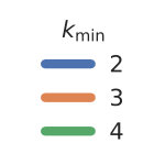 Figure 33
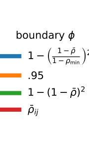 Figure 34
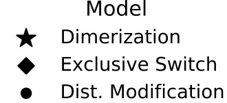 Figure 35
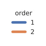 Figure 36
 Figure 37
 Figure 38
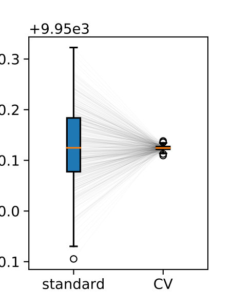 Figure 39
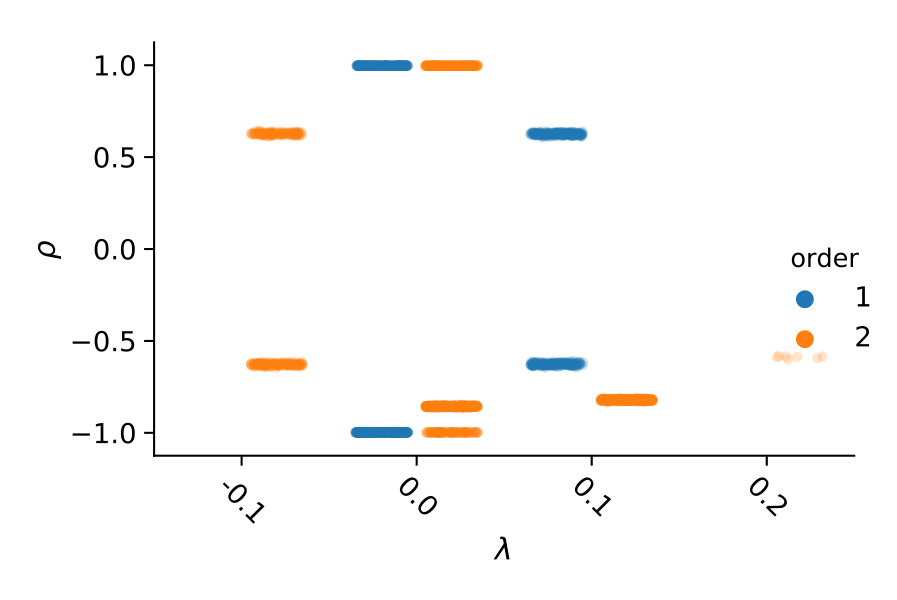 Figure 40
| Case study | slowdown | efficiency | ||||
|---|---|---|---|---|---|---|
| Dimerization | 10 | 0.881641 | 1.530137 | 5.558692 | 1.621917 | |
| 0.965224 | 1.945588 | 14.859417 | 3.338501 | |||
| 0.916445 | 1.625232 | 7.409904 | 1.997045 | |||
| 0.868288 | 1.380344 | 5.529745 | 1.081152 | |||
| 20 | 0.941153 | 1.637272 | 10.437978 | 1.842971 | ||
| 0.964204 | 1.907999 | 14.747328 | 2.915082 | |||
| 0.947984 | 1.747519 | 11.072422 | 2.227250 | |||
| 0.931030 | 1.433401 | 10.169570 | 1.088572 | |||
| 30 | 0.959517 | 1.723449 | 14.404936 | 1.972426 | ||
| 0.962514 | 1.770936 | 15.142156 | 2.216103 | |||
| 0.966216 | 1.847441 | 16.117387 | 2.446661 | |||
| 0.945724 | 1.456432 | 12.710196 | 1.084188 | |||
| Dist. mod. | 10 | 0.619560 | 1.488483 | 1.770218 | 3.232575 | |
| 0.700255 | 2.241695 | 1.492171 | 8.008607 | |||
| 0.643550 | 1.613001 | 1.743500 | 3.817641 | |||
| 0.596650 | 1.459405 | 1.703170 | 2.657000 | |||
| 20 | 0.697414 | 1.519425 | 2.181687 | 2.631677 | ||
| 0.713445 | 2.706546 | 1.292838 | 10.295856 | |||
| 0.697654 | 1.585313 | 2.092817 | 3.398235 | |||
| 0.695846 | 1.473976 | 2.235418 | 2.226530 | |||
| 30 | 0.712941 | 1.543068 | 2.263644 | 2.378037 | ||
| 0.721354 | 2.874249 | 1.252541 | 10.910880 | |||
| 0.711877 | 1.607712 | 2.164485 | 2.979704 | |||
| 0.669963 | 1.522184 | 1.996300 | 2.085473 | |||
| Excl. switch | 10 | 0.807184 | 1.227471 | 4.239255 | 2.536479 | |
| 0.880285 | 1.633530 | 5.135205 | 7.411732 | |||
| 0.849082 | 1.312416 | 5.067770 | 3.639250 | |||
| 0.783459 | 1.195821 | 3.874778 | 2.090101 | |||
| 20 | 0.856593 | 1.263340 | 5.539683 | 2.206154 | ||
| 0.910480 | 1.864405 | 6.011256 | 9.441336 | |||
| 0.867987 | 1.317958 | 5.765884 | 3.140806 | |||
| 0.825518 | 1.243075 | 4.627662 | 1.981143 | |||
| 30 | 0.869165 | 1.298893 | 5.905196 | 2.059415 | ||
| 0.921019 | 1.966191 | 6.461331 | 9.928998 | |||
| 0.876822 | 1.340409 | 6.079876 | 2.762449 | |||
| 0.843288 | 1.288925 | 4.968796 | 1.983174 |
| Case study | slowdown | efficiency | ||||
|---|---|---|---|---|---|---|
| Dimerization | 10 | 0.905254 | 1.659799 | 6.402491 | 2.388472 | |
| 0.987526 | 2.474939 | 33.074955 | 6.501180 | |||
| 0.923063 | 1.822654 | 7.195544 | 3.179257 | |||
| 0.878232 | 1.415909 | 5.830248 | 1.092264 | |||
| 20 | 0.949038 | 1.831995 | 10.797164 | 2.890898 | ||
| 0.985710 | 2.391457 | 29.704344 | 5.450299 | |||
| 0.968076 | 2.021487 | 15.662368 | 3.681229 | |||
| 0.925413 | 1.449386 | 9.298961 | 1.072761 | |||
| 30 | 0.964855 | 1.924268 | 14.911787 | 3.026275 | ||
| 0.981507 | 2.144089 | 25.520987 | 4.179125 | |||
| 0.973902 | 2.095985 | 18.507746 | 3.685851 | |||
| 0.948349 | 1.507425 | 12.904707 | 1.074538 | |||
| Dist. mod. | 10 | 0.619450 | 1.734737 | 1.519168 | 3.148184 | |
| 0.665361 | 3.301159 | 0.909443 | 13.456259 | |||
| 0.680592 | 1.840457 | 1.705876 | 3.864240 | |||
| 0.612674 | 1.662962 | 1.556868 | 2.659592 | |||
| 20 | 0.684789 | 1.811408 | 1.755652 | 2.687379 | ||
| 0.689835 | 4.455005 | 0.726640 | 17.609554 | |||
| 0.687665 | 1.901258 | 1.688449 | 3.413595 | |||
| 0.651262 | 1.770238 | 1.623924 | 2.266729 | |||
| 30 | 0.690602 | 1.922217 | 1.686011 | 2.375455 | ||
| 0.649191 | 4.837419 | 0.591701 | 19.145054 | |||
| 0.701253 | 2.001179 | 1.677062 | 3.007525 | |||
| 0.639123 | 1.894074 | 1.467403 | 2.086275 | |||
| Excl. switch | 10 | 0.811956 | 1.505521 | 3.544783 | 2.323999 | |
| 0.916866 | 4.507566 | 2.681363 | 21.692390 | |||
| 0.868874 | 1.776190 | 4.309354 | 4.739893 | |||
| 0.795802 | 1.466579 | 3.353046 | 2.016196 | |||
| 20 | 0.832562 | 1.657484 | 3.617313 | 2.085711 | ||
| 0.934280 | 6.348223 | 2.406431 | 29.976320 | |||
| 0.878944 | 1.879341 | 4.416281 | 3.990881 | |||
| 0.837922 | 1.647329 | 3.759896 | 1.978017 | |||
| 30 | 0.829427 | 1.844766 | 3.190308 | 2.043201 | ||
| 0.947324 | 7.130628 | 2.673225 | 32.513670 | |||
| 0.878830 | 2.053317 | 4.034987 | 3.611746 | |||
| 0.824936 | 1.838879 | 3.118728 | 1.978836 |
Peer Reviews
No public reviews on file for this paper yet. If you reviewed it on a platform where reviews are public (OpenReview, ICLR, NeurIPS, ICML), you can paste yours below so the community can read it here.
Videos
No videos yet. Explain this paper in a talk, walkthrough, or lecture? Add one.
11institutetext: 1Saarland University, Germany, 2University of Trieste, Italy
Control Variates for Stochastic Simulation
of Chemical Reaction Networks
Michael Backenköhler1
Luca Bortolussi1,2
Verena Wolf1
Abstract
Stochastic simulation is a widely used method for estimating quantities in models of chemical reaction networks where uncertainty plays a crucial role. However, reducing the statistical uncertainty of the corresponding estimators requires the generation of a large number of simulation runs, which is computationally expensive. To reduce the number of necessary runs, we propose a variance reduction technique based on control variates. We exploit constraints on the statistical moments of the stochastic process to reduce the estimators’ variances. We develop an algorithm that selects appropriate control variates in an on-line fashion and demonstrate the efficiency of our approach on several case studies.
Keywords:
Chemical Reaction Network Chemical Master Equation Stochastic Simulation Algorithm Moment Equations Control Variates Variance Reduction
1 Introduction
Chemical reaction networks that are used to describe cellular processes are often subject to inherent stochasticity. The dynamics of gene expression, for instance, is influenced by single random events (e.g. transcription factor binding) and hence, models that take this randomness into account must monitor discrete molecular counts and reaction events that change these counts. Discrete-state continuous-time Markov chains have successfully been used to describe networks of chemical reactions over time that correspond to the basic events of such processes. The time-evolution of the corresponding probability distribution is given by the chemical master equation, whose numerical solution is extremely challenging because of the enormous size of the underlying state-space.
Analysis approaches based on sampling, such as the Stochastic Simulation Algorithm (SSA) [18], can be applied independent of the size of the model’s state-space. However, statistical approaches are costly since a large number of simulation runs is necessary to reduce the statistical inaccuracy of estimators. This problem is particularly severe if reactions occur on multiple time scales or if the event of interest is rare. A particularly popular technique to speed up simulations is -leaping which applies multiple reactions in one step of the simulation. However, such multi-step simulations rely on certain assumptions about the number of reactions in a certain time interval. These assumptions are typically only approximately fulfilled and therefore introduce approximation errors on top of the statistical uncertainty of the considered point estimators.
Moment-based techniques offer a fast approximation of the statistical moments of the model. The exact moment dynamics can be expressed as an infinite-dimensional system of ODEs, which cannot be directly integrated for a transient analysis. Hence, ad-hoc approximations need to be introduced, expressing higher order moments as functions of lower-order ones [1, 13]. However, moment-based approaches rely on assumptions about the dynamics that are often not even approximately fulfilled and may lead to high approximation errors. Recently, equations expressing the moment dynamics have also been used as constraints for parameter estimation [5] and for computing moment bounds using semi-definite programming [12, 15].
In this work, we propose a combination of such moment constraints with the SSA approach. Specifically, we interpret these constraints as random variables that are correlated with the estimators of interest usually given as functions of chemical population variables. These constraints can be used as (linear) control variates in order to improve the final estimate and reduce its variance [23, 34]. The method is easy on an intuitive level: If a control variate is positively correlated with the function to be estimated then we can use the estimate of the variate to adjust the target estimate.
The incorporation of control variates into the SSA introduces additional simulation costs for the calculation of the constraint values. These values are integrals over time, which we accumulate based on the piece-wise constant trajectories. This introduces a trade-off between the variance reduction that is achieved by using control variates versus the increased simulation cost. This trade-off is expressed as the product of the variance reduction ratio and the cost increase ratio.
For a good trade-off, it is crucial to find an appropriate set of control variates. Here we propose a class of constraints which is parameterized by a moment vector and a weighting parameter, resulting in infinitely many choices. We present an algorithm that samples from the set of all constraints and proceeds to remove constraints that are either only weakly correlated with the target function or are redundant in combination with other constraints.
In a case study, we explore different variants of this algorithm both in terms of generating the initial constraint set and of removing weak or redundant constraints. We find that the algorithm’s efficiency is superior to a standard estimation procedure using stochastic simulation alone in almost all cases.
Although in this work we focus on estimating first order moments at fixed time points, the proposed approach can in principle deal with any property that can be expressed in terms of expected values such as probabilities of complex path properties. Another advantage of our technique is that an increased efficiency is achieved without the price of an additional approximation error as it is the case for methods based on moment approximations or multi-step simulations.
This paper is structured as follows. In Section 2 we give a brief survey of methods and tools related to efficient stochastic simulation and moment techniques. In Section 3 we introduce the common stochastic semantics of chemical reaction networks. From these semantics we show in Section 4 how to derive constraints on the moments of the transient distribution. The variance reduction technique of control variates is described in Section 5. We show the design of an algorithm using moment constraints to reduce sample variance in Section 6. The efficiency and other characteristics of this algorithm are evaluated on four non-trivial case studies in Section 7. Finally, we discuss the findings and give possibilities for further work in Section 8.
2 Related Work
Much research has been directed at the efficient analysis of stochastic chemical reaction networks. Usually research focuses on improving efficiency by making certain approximations.
If the state-space is finite and small enough one can deal with the underlying Markov chain directly. But there are also cases where the transient distribution has an infinitely large support and one can still deal with explicit state probabilities. To this end, one can fix a finite state-space, that should contain most of the probability [27]. Refinements of the method work dynamically and adjust the state-space according to the transient distributions [3, 20, 26].
On the other end of the spectrum there are mean-field approximations, which model the mean densities faithfully in the system size limit [6]. In between there are techniques such as moment closure [32], that not only consider the mean, but also the variance and other higher order moments. These methods depend on ad-hoc approximations of higher order moments to close the ODE system given by the moment equations. Yet another class of methods approximate molecular counts continuously and approximate the dynamics in such a continuous space, e.g. the system size expansion [35] and the chemical Langevin equation [16].
While the moment closure method uses ad-hoc approximations for high order moments to facilitate numerical integration, they can be avoided in some contexts. For the equilibrium distribution, for example, the time-derivative of all moments is equal to zero. This directly yields constraints that have been used for parameter estimation at steady-state [5] and bounding moments of the equilibrium distribution using semi-definite programming [14, 15, 21]. The latter technique of bounding moments has been successfully adapted in the context of transient analysis [12, 29, 30]. We adapt the constraints proposed in these works to improve statistical estimations via stochastic simulation (cf. section 4).
While the above techniques give a deterministic output, stochastic simulation generates single executions of the stochastic process [18]. This necessitates accumulating large numbers of simulation runs to estimate quantities. This adds a significant computational burden. Consequently, some effort has been directed at lowering this cost. A prominent technique is -leaping [17], which in one step performs multiple instead of only a single reaction. Another approach is to find approximations that are specific to the problem at hand, such as approximations based on time-scale separations [8, 7].
Recently, multilevel Monte Carlo methods have been applied in to time-inhomogenous CRNs [2]. In this techniques estimates are combined using estimates of different approximation levels.
The most prominent application of a variance reduction technique in the context of stochastic reaction networks is importance sampling [22]. This technique relies on an alteration of the process and then weighting samples using the likelihood-ratio between the original and the altered process.
3 Stochastic Chemical Kinetics
A chemical reaction network (CRN) describes the interactions between a set of species in a well-stirred reactor. Since we assume that all reactant molecules are spatially uniformly distributed, we just keep track of the overall amount of each molecule. Therefore the state-space is given by . These interactions are expressed a set of reactions with a certain inputs and outputs, given by the vectors and for reaction , respectively. Such reactions are denoted as
[TABLE]
The reaction rate constant gives us information on the propensity of the reaction. If just a constant is given, mass-action propensities are assumed. In a stochastic setting for some state these are
[TABLE]
The system’s behavior is described by a stochastic process . The propensity function gives the infinitesimal probability of a reaction occurring, given a state . That is, for a small time step
[TABLE]
This induces a corresponding continuous-time Markov chain (CTMC) on with generator matrix111Assuming a fixed enumeration of the state space.
[TABLE]
Accordingly, the time-evolution of the process’ distribution, given an initial distribution , is given by the Kolmogorov forward equation, i.e. , where . For a single state, it is commonly referred to as the chemical master equation (CME)
[TABLE]
A direct solution of (5) is usually not possible. If the state-space with non-negligible probability is suitably small, a state space truncation could be performed. That is, (5) is integrated on a possibly time-dependent subset [20, 27, 33]. Instead of directly analyzing (5), one often resorts to simulating trajectories. A trajectory over the interval is a sequence of states and corresponding jump times , and . We can sample trajectories of by using stochastic simulation [18].
Consider the birth-death model below as an example.
Model 1** (Birth-death process)**
A single species has a constant production and a decay that is linear in the current amount of molecules. Therefore the model consists of two mass-action reactions
[TABLE]
where denotes no reactant or no product, respectively.
For Model 1 the change of probability mass in a single state is described by expanding (5) and
[TABLE]
We can generate trajectories of this model by choosing either reaction, with a probability that is proportional to its rate given the current state . The jump time is determined by sampling from an exponential distribution with rate .
4 Moment Constraints
The time-evolution of for some function can be directly derived from (5) by computing the sum
[TABLE]
which yields
[TABLE]
While many choices of are possible, for this work we will restrict ourselves to monomial functions , i.e. the non-central moments of the process. The order of a moment is the sum over the exponents, i.e. . The integration of (6) with such functions is well-known in the context of moment approximations of CRN models. For most models the arising ODE system is infinitely large, because the time-derivative of low order moments usually depends on the values of higher order moments. To close this system, moment closures, i.e. ad-hoc approximations of higher order moments are applied [31]. The main drawback of this kind of analysis is that it is not known whether the chosen closure gives an accurate approximation for the case at hand. Here, such approximations are not necessary, since we will apply the moment dynamics in the context of stochastic sampling instead of trying to integrate (6).
Apart from integration strategies, setting (6) to zero has been used as a constraint for parameter estimation at steady-state [5] and bounding moments at steady-state [11, 15, 21]. The extension of the latter has recently lead to the adaption of these constraints to a transient setting [12, 30]. These two transient constraint variants are analogously derived by multiplying (6) by a time-dependent, differentiable weighting function and integrating:
Multiplying with and integrating on yields [12, 30]
[TABLE]
In the context of computing moment bounds via semi-definite programming the choices [30] and [12] have been proposed. While both choices proved to be effective in different case studies, relying solely on the latter choice, i.e. was sufficient.
By expanding the rate functions and in (7) and substituting the exponential weight function we can re-write (7) as
[TABLE]
with coefficients and vectors defined accordingly. Assuming the moments remain finite on , we can define the random variable
[TABLE]
with .
Note, that a realization of depends on the whole trajectory over . Thus, for the integral terms in (9) we have to compute sums
[TABLE]
over a given trajectory. This accumulation is best done during the simulation to avoid storing the whole trajectory. Still, the cost of a simulation run increases. For the method to be efficient, the variance reduction (Section 5) needs to overcompensate for this increased cost of a simulation run.
For Model 1 the moment equation for becomes
[TABLE]
The corresponding constraint (8) with gives
[TABLE]
In this instance the constraint leads to an explicit function of the moment over time. If w.p. 1, then (8) becomes
[TABLE]
when choosing .
5 Control Variates
Now, we are interested in the estimation of some quantity by stochastic simulation. Let be independent samples of . Then the sample mean is an estimate of . By the central limit theorem
[TABLE]
Now suppose, we know of a random variable with . The variable is called a control variate. If a control variate is correlated with , we can use it to reduce the variance of [19, 28, 34, 36]. For example, consider we are running a set of simulations and consider a single constraint. If the estimated value of this constraint is larger than zero and we estimate a positive correlation between the constraint and , we would, intuitively, like to decrease our estimate accordingly. This results in an estimation of the mean of the random variable
[TABLE]
instead of . The variance
[TABLE]
The optimal choice can be computed by considering the minimum of . Then
[TABLE]
Therefore , where is the correlation of and .
If we have multiple control variates, we can proceed in a similar fashion. Now, let denote a vector of control variates and let
[TABLE]
be the covariance matrix of . As above, we estimate the mean of The ideal choice of is the result of an ordinary least squares regression between and , . Specifically, . Then, asymptotically the variance of this estimator is [34],
[TABLE]
In practice, however, is unknown and needs to be replaced by an estimate . This leads to an increase in the estimator’s variance. Under the assumption of and having a multivariate normal distribution [10, 23], the variance of the estimator is
[TABLE]
Clearly, a control variate is “good” if it is highly correlated with . The constraint in (11) is an example of the extreme case. When we use this constraint as a control variate for the estimation of the mean at some time point , it has a correlation of since it describes the mean at that time precisely. Therefore the variance is reduced to zero. We thus aim to pick control variates that are highly correlated with .
Consider, for example, the above case of the birth-death process. If we choose (11) as a constraint, it would always yield the exact difference of the exact mean to the sample mean and therefore have a perfect correlation. Clearly, reduces to 1 and .
6 Moment-Based Variance Reduction
We propose an adaptive estimation algorithm (Algorithm 1) that starts out with an initial set of control variates and periodically removes potentially inefficient variates. The “accumulator set” represents the time-integral terms (10). The size of has the most significant impact on the overall speed of the algorithm since it represents the only factor incurring a direct cost increase in the SSA itself (line 5).
The algorithm consists of a main loop which performs simulation runs (line 4). Between each run the mean and covariance estimates of are updated (line 6). Every iterations, the control variates are checked for efficiency and redundancy (lines 7–12).
Checking both conditions is based on the correlation between the -th and -th control variate and the correlation of a control variate to . The first condition is a simple lower threshold for a correlation . This condition aims to remove those variates from the control variate set that are only weakly correlated to (line 9). The rationale is that, if variate has a low correlation with the variable of interest , its computation may not be worth the costs. Here, we propose to set heuristically as
[TABLE]
where is an algorithm parameter.
The second condition aims to remove redundant conditions. This is not only beneficial for the efficiency of the estimator, but also necessary for the matrix inversion (12) because perfectly and highly correlated constraints will make the covariance matrix estimate (quasi-) singular. For all considered criteria we iterate over all tuples , , removing the weaker of the two, i.e. , if the two control variates are considered redundant (line 10).
There are many ways to define such a redundancy criterion. Here, we focus on criteria that are defined in terms of the average correlation . For two variates and we then check if their mutual correlation exceeds a some function of , i.e. we check the inequality
[TABLE]
If this inequality holds, constraint is removed. Naturally, there are many possible choices for the above decision boundary (cf. Fig. 1a).
The simplest choice is to ignore and just fix a constant close to 1 as a threshold, e.g. . While this often leads to the strongest variance reduction and avoids numerical issues in the control variate computation, it turns out that the computational overhead is not as well-compensated as by other choices of (see Section 7).
Another option is to fix a simple linear function, i.e. . For this choice the intuition is, that one of two constraints is removed if their mutual correlation exceeds their average correlation with .
Here, we also assess two quadratic choices for . The first choice of is more tolerant than the linear function and more strict than a threshold function, except for highly correlated control variates. Another variant of is given by including the lower bound and scaling the quadratic function accordingly: . The different choices of considered here are plotted in Figure 1a.
Now, we discuss the choice of the initial control variates. We identify control variate by a tuple of a moment vector and a time-weighting parameter . That is, we use and in (7). For a given set of parameters , we use all moments up to some fixed order (line 3). The ideal set of parameters is generally not known. For certain choices the correlation of the control variates and the variable of interest is higher then for others. To illustrate this, consider the above example of the birth-death process. Choosing leads to a control variate that has a correlation of with . Therefore, the ideal choice of initial values for would be . This, however, is generally not known. Therefore, we sample a set of ’s from some fixed distribution (line 2).
7 Case Studies
We first define a criterion of efficiency in order to estimate whether the reduction in variance is worth the increased cost. A natural baseline of a variance reduction is, that it is more efficient to pay for the overhead of the reduction than to generate more samples to achieve a similar reduction of variance. Let be the variance of . The efficiency of the method is the ratio of the necessary cost to achieve a similar reduction with the CV estimate compared to the standard estimate [24], i.e.
[TABLE]
That ratio depends on both the specific implementation and the technical setup. The cost increase is mainly due to the computation of the integrals in (8). But the repeated checking of control variates for efficiency also increases the cost. The accumulation over the trajectory directly increases the cost of a single simulation which is the critical part of the estimation. To estimate the base-line cost , 2000 estimations were performed without considering any control variates.
The simulation is implemented in the Rust programming language222https://www.rust-lang.org. The model description is parsed from a high level specification. Rate functions are compiled to stack programs for fast evaluation. Code is made available online [4].
We consider four non-trivial case studies. Three models exhibit complex multi-modal behaviour. We now describe the models and the estimated quantities in detail.
The first model is a simple dimerization on a countably infinite state-space.
Model 2** (Dimerization)**
We first examine a simple dimerization model on an unbounded state-space
[TABLE]
with initial condition .
Despite the models simplicity, the moment equations are not closed for this system due to the second reaction which is non-linear. Therefore a direct analysis of the expected value would require a closure. For this model we will estimate .
The following two models are bimodal, i.e. they each posses two stable regimes among which they can switch stochastically. For both models we choose the initial conditions such that the process will move towards either attracting region with equal probability.
Model 3** (Distributive Modification)**
The distributive modification model was introduced in [9]. It consists of the reactions
[TABLE]
with initial conditions .
Model 4** (Exclusive Switch)**
The exclusive switch model consists of 5 species, 3 of which are typically binary (activity states of the genes) [25].
[TABLE]
with initial conditions and .
We evaluate the influence of algorithm parameters, choices of distributions to sample from, and the influence of the sample size on the efficiency of the proposed method. Note that the implementation does not simplify the constraint representations or the state space according to stoichiometric invariants or limited state spaces. Model 3, for example has the invariant , , which could be used to reduce the state-space dimensionality to two. In Model 4 the invariant could be used to optimize the algorithm by eliminating redundant moments, e.g. . Such an optimization would further increase the efficiency of the algorithm.
We first turn to the choice of the sampling distribution. Here we consider two choices:
a standard normal distribution , 2. 2.
a uniform distribution on .
We deterministically include in the constraint set, as this parameter corresponds to a uniform weighting function. We performed estimations on the case studies using different valuations of the algorithm parameters of the minimum threshold and the number of -samples . We used samples size and checked the control variates every iterations for the defined criteria. For each valuation 1000 estimations were performed. In Figure 2b, we summarize the efficiencies for the arising parameter combinations on the three case studies. Most strikingly, we can note that the efficiency was consistently larger than one in all cases. Generally, the normal sampling distribution out-performed the alternative uniform distribution, except in case of the dimerization. The reason for this becomes apparent, when examining Figure 1b,c: In case of the dimerization model the most efficient constraints are found for , while in case of the distributive modification they are located just above 0 (we observe a similar pattern for the exclusive switch case study). Therefore the sampling of efficient values is more likely using a uniform distribution for the dimerization case study, than it is for the others. Given that larger absolute values for seem unreasonable due their exponential influence on the weighting function and the problem of fixing a suitable interval for a uniform sampling scheme, the choice of a standard normal distribution for seems superior.
In Figure 3 we compare efficiencies for different maximum orders of constraints . This comparison is performed for different choices of the redundancy rule and initial sample sizes . Again, for each parameter valuation 1000 estimations were performed. With respect to the maximum constraints order we see a clear tendency, that the inclusion of second order constraints lessens the efficiency of the method. In case of a constant redundancy threshold it even dips below break-even for the distributive modification case study. This is not surprising, since the inclusion of second order moments increases the number of initial constraints quadratically and the incurred cost, especially of the first iterations, lessens efficiency.
Figure 4 depicts the trade-off between the variance reduction versus the cost ratio . Comparing the redundancy criterion based on a constant threshold to the others, we observe both a larger variance reduction and an increased cost. This is due to the fact, that more control variates are included throughout the simulations (cf. Appendix 0.A, Tables 1,2). Depending on the sample distribution and the case study, this permissive strategy may pay off. In case of the dimerization, for example, it pays off, while in case of the distributive modification it leads to a lower efficiency ratio. In the latter case the model is more complex, and therefore the set of initial control variates is larger. With a more permissive redundancy strategy, more control variates are kept (ca. 10 when using vs. ca. 2–3 for the others). The other redundancy boundaries move the results further in the direction of less variance reduction while keeping the cost increase low. On the opposite end is the linear . The quadratic versions and can be found in the middle of this spectrum.
We also observe, that an increase of is particularly beneficial, if the sampling distribution does not capture the parameter region of the highest correlations well. This can be seen for the Dimerization case study, where the variance reduction increases strongly with increasing sample size (App. 0.A Tables 1,2). Since , more samples are needed to sample efficient -values (cf. Figure 1b).
Finally, we discuss the effect of the sample size on the efficiency . In Figure 5 we give both the efficiencies and the slowdown for different sample sizes. As a redundancy rule we used the unscaled quadratic function, 30 initial values of , and . With increasing sample size, the efficiency usually approaches an upper limit. This is due to the fact that most control variates are dropped early on and the control variates often remain the same for the rest of the simulations. If we assume there are no helpful control variates in the initial set and all would be removed at iteration 100, the efficiency would approach 1 with .
8 Conclusion
In this work we have shown that known constraints on the moment dynamics can be successfully leveraged in simulation-based estimation of expected values. The empirical results indicate that the supplementing a standard SSA estimation with moment information can drastically reduce the estimators’ variance. This reduction is paid for by accumulating information on the trajectory during simulation. However, the reduction is able to compensate for this increase. This means that for fixed costs, using estimates with control variates is more beneficial than using estimates without control variates.
While a variety of algorithmic variants was evaluated, many aspects remain subject to further study. In particular different choices of and in (7) may improve efficiency further. These choices become particularly interesting when moving from the estimation of simple first order moments to more complex queries such as behavioural probabilities of trajectories. In such cases, one might even attempt to find efficient control variate functions using machine learning methods.
Another open question regarding this work is its performance when multiple quantities instead of a single quantity are to be estimated. In such a case, constraints would be particularly beneficial, if they lead to improvements as many estimation targets as possible.
Furthermore the identification of the best weighting parameters could be done in a more adaptive fashion. The presented scheme of a sampling from could be extended into a Bayesian-like procedure, wherein the values for are periodically re-sampled from a distribution that is adjusted according to the best-performing constraints up to that point.
8.0.1 Acknowledgements
This work was supported by the DFG project MULTIMODE.
Appendix 0.A Supplementary Material
In Figure 6 we give detailed information on the influence of algorithm parameters , the number of initial values, and different redundancy rules. The sampling distribution is a standard normal.
The reference list from the paper itself. Each links out to its DOI / PubMed record.
- 1[1] Ale, A., Kirk, P., Stumpf, M.P.: A general moment expansion method for stochastic kinetic models. The Journal of chemical physics 138 (17), 174101 (2013)
- 2[2] Anderson, D.F., Yuan, C.: Low variance couplings for stochastic models of intracellular processes with time-dependent rate functions. Bulletin of mathematical biology pp. 1–29 (2018)
- 3[3] Andreychenko, A., Mikeev, L., Spieler, D., Wolf, V.: Parameter identification for markov models of biochemical reactions. In: International Conference on Computer Aided Verification. pp. 83–98. Springer (2011)
- 4[4] Backenköhler, M.: Cme stochastic simulation code. https://github.com/mbackenkoehler/cme-simulation (2019)
- 5[5] Backenköhler, M., Bortolussi, L., Wolf, V.: Moment-based parameter estimation for stochastic reaction networks in equilibrium. IEEE/ACM Transactions on Computational Biology and Bioinformatics (TCBB) 15 (4), 1180–1192 (2018)
- 6[6] Bortolussi, L., Hillston, J., Latella, D., Massink, M.: Continuous approximation of collective system behaviour: A tutorial. Performance Evaluation 70 (5), 317–349 (2013)
- 7[7] Bortolussi, L., Milios, D., Sanguinetti, G.: Efficient stochastic simulation of systems with multiple time scales via statistical abstraction. In: International Conference on Computational Methods in Systems Biology. pp. 40–51. Springer (2015)
- 8[8] Cao, Y., Gillespie, D.T., Petzold, L.R.: The slow-scale stochastic simulation algorithm. The Journal of chemical physics 122 (1), 014116 (2005)