Lifting Vectorial Variational Problems: A Natural Formulation based on Geometric Measure Theory and Discrete Exterior Calculus
Thomas M\"ollenhoff, Daniel Cremers

TL;DR
This paper introduces a novel convex formulation for vectorial variational problems in imaging by lifting them to the space of currents and discretizing with Whitney forms, enabling more effective shape optimization.
Contribution
It presents a new convex relaxation approach for vector-valued variational problems using geometric measure theory and discrete exterior calculus, extending multilabeling methods.
Findings
Convex relaxation via currents improves problem tractability.
Discretization with Whitney forms generalizes multilabeling approaches.
The method facilitates shape optimization in imaging tasks.
Abstract
Numerous tasks in imaging and vision can be formulated as variational problems over vector-valued maps. We approach the relaxation and convexification of such vectorial variational problems via a lifting to the space of currents. To that end, we recall that functionals with polyconvex Lagrangians can be reparametrized as convex one-homogeneous functionals on the graph of the function. This leads to an equivalent shape optimization problem over oriented surfaces in the product space of domain and codomain. A convex formulation is then obtained by relaxing the search space from oriented surfaces to more general currents. We propose a discretization of the resulting infinite-dimensional optimization problem using Whitney forms, which also generalizes recent "sublabel-accurate" multilabeling approaches.
Click any figure to enlarge with its caption.
 Figure 1
 Figure 2
 Figure 3
 Figure 4
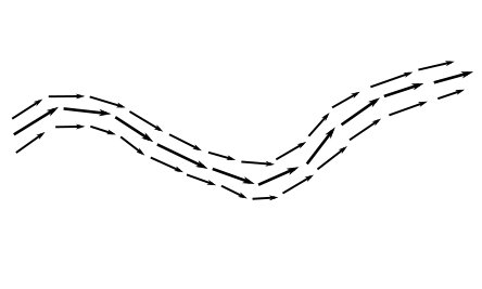 Figure 5
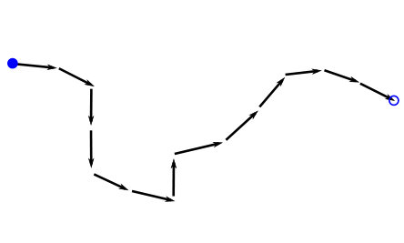 Figure 6
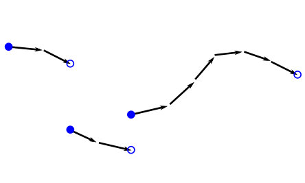 Figure 7
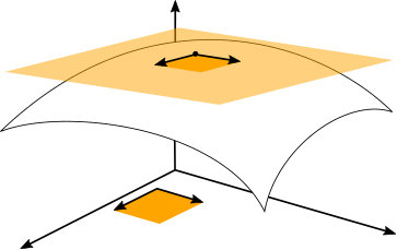 Figure 8
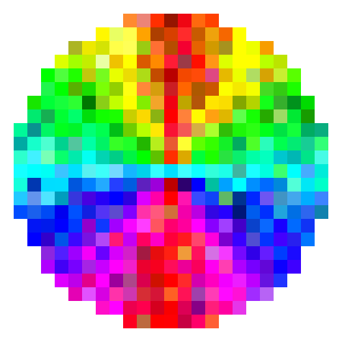 Figure 9
 Figure 10
 Figure 11
 Figure 12
 Figure 13
 Figure 14
 Figure 15
 Figure 16
Peer Reviews
No public reviews on file for this paper yet. If you reviewed it on a platform where reviews are public (OpenReview, ICLR, NeurIPS, ICML), you can paste yours below so the community can read it here.
Videos
No videos yet. Explain this paper in a talk, walkthrough, or lecture? Add one.
Lifting Vectorial Variational Problems: A Natural Formulation based on
Geometric Measure Theory and Discrete Exterior Calculus
Thomas Möllenhoff and Daniel Cremers
Technical University of Munich
{thomas.moellenhoff,cremers}@tum.de
Abstract
Numerous tasks in imaging and vision can be formulated as variational problems over vector-valued maps. We approach the relaxation and convexification of such vectorial variational problems via a lifting to the space of currents. To that end, we recall that functionals with polyconvex Lagrangians can be reparametrized as convex one-homogeneous functionals on the graph of the function. This leads to an equivalent shape optimization problem over oriented surfaces in the product space of domain and codomain. A convex formulation is then obtained by relaxing the search space from oriented surfaces to more general currents. We propose a discretization of the resulting infinite-dimensional optimization problem using Whitney forms, which also generalizes recent “sublabel-accurate” multilabeling approaches.
1 Introduction
We consider functionals of -mappings
[TABLE]
where , are bounded and open. The cost function is assumed to be a nonnegative (possibly nonconvex) continuous function on that is polyconvex (see Def. 2) in the Jacobian matrix .
This work is concerned with relaxation and global optimization of (1) when, both, dimension and codimension are possibly larger than one (, ). This is expected to be difficult: In the discrete setting problems with or typically correspond to polynomial-time solvable shortest path () or graph cut () problems [cohen1997global, tsitsiklis, Ishikawa, schoenemann2010combinatorial], whereas for , the arising multilabel problems with unordered label spaces are known to be NP-hard - see [li2016complexity]. Nevertheless, heuristic strategies have been shown to yield excellent results in tasks such as optical flow [fullflow] or shape matching [shekhovtsov2008efficient, chen2015robust]. In contrast to such well-established Markov random field (MRF) works [kolmogorov2006convergent, kolmogorov2007minimizing, kohli2008partial, shekhovtsov2008efficient, menze2015discrete, chen2015robust, fullflow, domokos2018mrf] we consider the way less explored continuous (infinite-dimensional) setting.
Our motivation partly stems from the fact that formulations in function space are very general and admit a variety of discretizations. Finite difference discretizations of continuous relaxations often lead to models that are reminiscent of MRFs [Zach-et-al-cvpr12], while piecewise-linear approximations are related to discrete-continuous MRFs [Zach-Kohli-eccv14], see [fix2014duality, moellenhoff-iccv-2017]. More recently, for the Kantorovich relaxation in optimal transport, approximations with deep neural networks were considered and achieved promising performance, for example in generative modeling [ACB17, seguy2017large].
We further argue that fractional (non-integer) solutions to a careful discretization of the continuous model can implicitly approximate an “integer” continuous solution. Therefore one can achieve accuracies that go substantially beyond the mesh size. The resulting models would be difficult to interpret and derive from a finite-dimensional viewpoint such that the continuous considerations are required for the final implementation. Also, formulations arising from continuous relaxations allow one to introduce isotropic smoothness potentials without reverting to higher-order terms in the cost, and, as we show in this work, one can impose general polyconvex regularizations using only local constraints. An example of a polyconvex function (which is in general nonconvex) is the surface area of the graph, sometimes referred to as “Beltrami regularization” in the image processing community, see e.g., [belt].
In contrast to the discrete multi-labeling setting, an important question is whether variational problems involving the energy (1) admit a minimizer. A fruitful approach to address this question is to suitably relax the notion of solution, thereby enlarging the search space of admissible candidates (“lifting the problem to a larger space”). The origins of this idea can be traced back111We refer the interested reader to the historical remarks in L. C. Young’s book on the calculus of variations [young2000lecture, pp. 122–123]. to the turn of the century, see Hilbert’s twentieth problem [hilbert]. An example of that principle is the celebrated Kantorovich relaxation [kantorovich1960] of Monge’s transportation problem [monge1781]. There, the search over maps is relaxed to one over probability measures on the product space . Each map can be identified in that extended space with a measure concentrated on its graph. Existence of optimal transportation plans follows directly due to good compactness properties of the larger space. Furthermore, the nonlinearly constrained and nonconvex optimization problem is transformed into one of linear programming, leading to rich duality theories and fast numerical algorithms [PeCu18].
One may ask whether the relaxed solution in the extended space has certain regularity properties, for example whether it is the graph of a (sufficiently regular) map and thus can be considered a solution to the original (“unlifted”) problem. In the case of optimal transport, such regularity theory can be guaranteed under some assumptions [Vil08, San15]. Establishing existence and regularity for problems in which the cost additionally depends on the Jacobian (for example minimal surface problems) has been a driving factor in the development of geometric measure theory, see [morgan2016geometric] for an introduction. In this work, we will use ideas from geometric measure theory to pursue the above relaxation and lifting principle for the energy (1). The main idea is to reformulate the original variational problem as a shape optimization problem over oriented manifolds representing the graph of the map in the product space . To obtain a convex formulation we enlarge the search space from oriented manifolds to currents.
1.1 Related Work
A common strategy to solve problems involving (1) is to revert to local gradient descent minimization based on the Euler-Lagrange equations. But for nonconvex problems solutions might depend on the initialization and the computed stationary points may be quite suboptimal. Therefore, we pursue the aforementioned lifting of the energy (1) to currents. This lifting has been previously considered in geometric measure theory to establish the aforementioned existence and regularity theory for vectorial variational problems in a very broad setting, see e.g., [federer, federer1974real, aviles1991variational]. In contrast to such impressive theoretical achievements, this paper is concerned with a discretization and implementation.
There is also a variety of related applied works. The paper [windheuser2011geometrically] tackles the problem of bijective and smooth shape matching using linear programming. Similar to the present work, the authors also look for graph surfaces in but they consider the discrete setting and use a different notion of boundary operator. We study the continuous setting, but also our discrete formulation is quite different.
For , the proposed continuous formulation specializes to [ABDM, PCBC-SIIMS]. To tackle the setting of in a memory efficient manner, Strekalovskiy et al. [Strekalovskiy-et-al-cvpr12, goldluecke2013tight, strekalovskiy-et-al-siims14] keep a collection of surfaces with codimension one under the factorization assumption that . In contrast, we consider only one surface of codimension , we do not require an assumption on , our approach is applicable to a larger class of functionals and we expect it to yield a tighter relaxation. The lifting approaches [lellmann-et-al-iccv2013, goldstein2012global] also tackle vectorial problems by considering the full product space, but are limited to total variation regularization (with the former allowing to be a manifold). The recent work [windheuser2016convex] is most related to the present one, however their relaxation considers a specific instance of (1). Moreover, the above works are based on finite difference discretizations of the continuous model. In contrast, the proposed discretization using discrete exterior calculus yields solutions beyond the mesh accuracy as in recent sublabel-accurate approaches. The latter are restricted to [moellenhoff-laude-cvpr-2016, moellenhoff-iccv-2017] or total variation regularization [laude16eccv]. Recent works also include extensions to total generalized variation or Laplacian regularization [strecke2018sublabel, vogt, loewe].
Recent approaches in shape analysis [solomon2016entropic, vestner2017product, vestner2017efficient] also operate in the product space . However, these are based on local minimizations of the Gromov-Wasserstein distance [memoli2007use] and spectral variants thereof [memoli2009spectral] which leads to (nonconvex) quadratic assignment problems. While the goal to find a smooth (possibly bijective) map is similar, the formulations appear to be quite different. To alleviate the increased cost of the product space formulation, computationally efficient representations of densities in have been studied in the context of functional maps [ovsjanikov2012functional, rodola2018functional].
2 Notation and Preliminaries
Throughout this paper we will introduce notions from geometric measure theory, as they are not commonly used in the vision community. While the subject is rather technical, our aim is to keep the presentation light and to focus on the geometric intuition and aspects which are important for a practical implementation. We invite the reader to consult chapter 4 in the book [morgan2016geometric] and the chapter on exterior calculus in [crane2015discrete], which both contain many illuminating illustrations. For a more technical treatment we refer to [federer, KP08].
In the following, we denote a basis in as with dual basis where is the linear functional that maps every to the -th component . Given an integer , are the multi-indices with .
As we will consider -surfaces in , most of the time we set and . To further simplify notation, we denote the basis vectors by and similarly refer to the dual basis as . When it is clear from the context, we treat vectors and in the sense that , . As an example, for we can define the expression and read it as .
2.1 Convex Analysis
The extended reals are denoted by . For a finite-dimensional real vector space and we denote the convex conjugate as and the biconjugate as . is the largest lower-semicontinuous convex function below . In our notation, for functions with several arguments, the conjugate is always taken only in the last argument. As a general reference to convex analysis, we refer the reader to the books [hiriart2012fundamentals, Rockafellar:ConvexAnalysis].
2.2 Multilinear Algebra
The formalism of multi-vectors we introduce in this section is central to this work, as the idea of the relaxation is to represent the oriented graph of by a -vectorfield (more precisely: a -current) in the product space . Basically, one can multiply to obtain an object
[TABLE]
called a simple -vector in . The geometric intuition of simple -vectors is, that they describe the -dimensional space spanned by the , together with an orientation and the area of the parallelotope given by the . Thus, simple -vectors can be thought of oriented parallelotopes as shown in orange in Fig. 1. In general, -vectors are defined to be formal sums
[TABLE]
for coefficients . They form the vector space , which has dimension .
The dual space of -covectors is defined analogously, with . We define for two -vectors (and also for -covectors) , an inner product and norm .
-vectors (elements of ) are called simple, if they can be written as the wedge product of -vectors as in (2). Unfortunately, for , not all -vectors are simple and the set of simple -vectors is a nonconvex cone in , called the Grassmann cone [busemann1963convex]. This is one aspect why the setting of and is more challenging.
Later on, we will consider a relaxation from the nonconvex set of simple -vectors to general -vectors. Naturally, for the relaxation to be good, we want the convex energy to be as large as possible on non-simple -vectors. For the Euclidean norm, a good convex extension is the mass norm
[TABLE]
The dual norm is the comass norm given by:
[TABLE]
The mass norm can be understood as the largest norm that agrees with the Euclidean norm on simple -vectors.
3 Lifting to Graphs in the Product Space
With the necessary preliminaries in mind, our goal is now to reparametrize the original energy (1) to the graph . As shown in Fig. 1, the graph is an oriented -dimensional manifold in the product space with global parametrization .
Definition 1** (Orientation).**
If is a -dimensional smooth manifold in (possibly with boundary), an orientation of is a continuous map such that is a simple -vector with unit norm that spans the tangent space at every point .
From differential geometry we know that the tangent space at is spanned by . Therefore, an orientation of is given by
[TABLE]
where the map is given by
[TABLE]
and is the canonical projection onto the first argument. In order to derive the reparametrization, we have to connect a simple -vector (representing an oriented tangent plane of the graph) with the Jacobian of the original energy. For that, we need an inverse of the map given in (7).
To derive such an inverse, we first introduce further helpful notations. For we denote by the element which complements in in increasing order, denote and [math] as the empty multi-index. Every can be written as
[TABLE]
where , , . To give an example, the coefficients of a -vector according to the notation (8) are:
[TABLE]
where we highlighted the coefficients with . Now note that the vector is by construction a simple -vector with first component . To any with we associate given by
[TABLE]
If and only if is simple with first component then . A proof is given in [GMS-CC, Vol. I, Ch. 2.1, Prop. 1]. Thus, on the set of simple -vectors with first component ,
[TABLE]
the inverse of the map (7) is given by (10).
Using the above notations, we can define a generalized notion of convexity, which essentially states that there is a convex reformulation on -vectors.
Definition 2** (Polyconvexity).**
A map is polyconvex if there is a convex function such that we have
[TABLE]
Equivalently one has that for all . We also refer to the convex function as a polyconvex extension.
In general, the polyconvex extension is not unique. Any convex function has an obvious polyconvex extension by (10), but as discussed in the previous section we would like the convex extension to be as large as possible for . The largest polyconvex extension which agrees with the original function on can be formally defined using the convex biconjugate, but is often hard to explicitly compute. The mass norm (4) corresponds to such a construction.
Nevertheless, given any polyconvex extension, we can now reparametrize the original energy (1) on the oriented graph , as we show in the following central proposition.
Proposition 1**.**
Let be a polyconvex extension of the original cost in the last argument. Define the function ,
[TABLE]
where and are the canonical projections onto the first and second argument. Then we can reparametrize (1) as follows:
[TABLE]
where the second integral is the standard Lebesgue integral with respect to the -dimensional Hausdorff measure on restricted to the graph .
Proof.
We directly calculate:
[TABLE]
The step from (15) to (16) uses that is a polyconvex extension (so that we can apply (12)) and the fact that for we have . To arrive at (17), an application of the area formula [KP08, Corollary 5.1.13] suffices and for (18) we used positive one-homogenity of and the definition of in (6). ∎
Interestingly, the function (13) is convex and one-homogeneous in the last argument, as it is the perspective of a convex function. However, the search space of oriented graphs of mappings is nonconvex. Therefore we relax from oriented graphs to the larger set of currents, which we will introduce in the following section. Since currents form a vector space, we therefore obtain a convex functional over a convex domain.
4 From Oriented Graphs to Currents
Throughout this section, let be an open set, which will later be a neighbourhood of , where , are the closures of . The main idea of our relaxation and the geometric intuitions of pushforward and boundary operator we introduce in this section are summarized in the following Fig. 2. Currents are defined in duality with differential forms, which we will briefly introduce in the following section.
4.1 Differential Forms
A differential form of order (short: -form) is a map . The support of a differential form is defined as the closure of . Integration of a -form over an oriented -dimensional manifold is defined by
[TABLE]
A notion of derivative for -forms is the exterior derivative , which is a -form given by:
[TABLE]
where is the oriented boundary of the parallelotope spanned by the at point .
To get an intuition, note that for this reduces to the familiar directional derivative . With (19) and (20) in mind, one sees why Stokes’ theorem
[TABLE]
should hold intuitively. Given a map , the pullback of the -form is determined by
[TABLE]
where and is the Jacobian.
4.2 Currents
Denote the space of smooth -forms with compact support on as . Currents are elements of the dual space , i.e., linear functionals acting on differential forms. As shown in Fig. 2(a), an oriented -dimensional manifold induces a current by
[TABLE]
However, since is a vector space, not all elements look like -dimensional manifolds, see Fig. 2(d). The boundary of the -current is the -current defined via the exterior derivative:
[TABLE]
Stokes’ theorem (21) ensures that for currents which are given by -dimensional oriented manifolds, the boundary of the current agrees with the usual notion, see Fig. 2(b).
The support of a current, denoted by , is the complement of the biggest open set such that
[TABLE]
Given a map the pushforward of the -current is given by
[TABLE]
Intuitively, it transforms the current using the map , as illustrated in Fig. 2(a). The mass of a current is
[TABLE]
and as expected . We denote the space of -currents with finite mass and compact support by . These are representable by integration, meaning there is a measure on and a map such that for -almost all such that
[TABLE]
The decomposition (28) is crucial, and we will use it to define the relaxation in the next section.
4.3 The Relaxed Energy
We lift the original energy (1) to the space of finite mass currents with as follows:
[TABLE]
Since for we have , \|T\|=\mathcal{H}^{n}\,\raisebox{-0.5468pt}{\reflectbox{\rotatebox[origin={br}]{-90.0}{\lnot}}}\,\mathcal{G}_{f} the desirable property holds due to Prop. 1.
Note that in (29) we use the lower-semicontinuous regularization which extends (13) at with the correct value. Interestingly, this point corresponds to the situation when the graph has vertical parts, which cannot occur for functions but can happen for general currents, see Fig. 2(c). In [Mora] it was shown that one can penalize such jumps in a way depending on the jump distance and direction. We will not consider such additional regularization due to space limitations, but remark that they could be integrated by adding further constraints to the following dual representation, which is a consequence of [GMS-CC, Vol. II, Sec. 1.3.1, Thm. 2].
Proposition 2**.**
For with , we have the dual representation
[TABLE]
where the constraint is the closed and convex set
[TABLE]
The final relaxed optimization problem for (1) reads
[TABLE]
Depending on the kind of problem one wishes to solve, a different convex constraint set should be considered. For example, in the case of variational problems with Dirichlet boundary conditions, we set
[TABLE]
where is a given boundary datum. In case of Neumann boundary conditions, one constrains the support of the boundary to be zero inside the domain
[TABLE]
to exclude surfaces with holes, but allow the boundary to be freely chosen on . In case , one can also consider the constraint set
[TABLE]
where the additional pushforward constraint encourages bijectivity. Notice also the similarity of (32) together with (35) to the Kantorovich relaxation in optimal transport.
Existence of minimizing currents to a similar problem as (32) in a certain space of currents (real flat chains) is shown in [federer1974real, §3.9]. For dimension or codimension , the infimum is actually realized by a surface (integral flat chain) [federer1974real, §5.10, §5.12]. An adaptation of such theoretical considerations to our setting and conditions under which the relaxation is tight in the scenario , is a major open challenge and left for future work.
5 Discrete Formulation
In this section we present an implementation of the continuous model (32) using discrete exterior calculus [Hirani2003]. We will base our discretization on cubes since they are easy to work with in high dimensions, but one could also use simplices. To define cubical meshes, we adopt some notations from computational homology [CH].
Definition 3** (Elementary interval and cube).**
An elementary interval is an interval of the form or for . Intervals that consist of a single point are degenerate. An elementary cube is given by a product , where each is an elementary interval. The set of elementary cubes in is denoted by .
For , denote by the number of nondegenerate intervals. We denote as the multi-index referencing the nondegenerate intervals.
Definition 4** (Cubical set).**
A set is a cubical set if it can be written as a finite union of elementary cubes.
Let be the set of -dimensional cubes contained in . A map will transform the cubical set to our domain. As we work with images, it will just be a mesh spacing, i.e., we set .
Definition 5** (-chains, -cochains).**
We denote the space of finite formal sums of elements in with real coefficients as , called (real) -chains. We denote the dual as and call the elements -cochains.