TL;DR
This paper analyzes the smoothness challenges in nonlinear system identification and proposes multiple shooting as a solution to improve optimization stability and feasibility in complex models.
Contribution
It introduces multiple shooting for nonlinear system identification, addressing smoothness issues and enabling estimation in chaotic or unstable systems.
Findings
Lipschitz constant and smoothness can grow exponentially with simulation length in non-contractive regions.
Multiple shooting improves optimization stability by splitting data into smaller subsets.
The method effectively estimates parameters of chaotic systems and neural networks.
Abstract
We shed new light on the \textit{smoothness} of optimization problems arising in prediction error parameter estimation of linear and nonlinear systems. We show that for regions of the parameter space where the model is not contractive, the Lipschitz constant and -smoothness of the objective function might blow up exponentially with the simulation length, making it hard to numerically find minima within those regions or, even, to escape from them. In addition to providing theoretical understanding of this problem, this paper also proposes the use of multiple shooting as a viable solution. The proposed method minimizes the error between a prediction model and the observed values. Rather than running the prediction model over the entire dataset, multiple shooting splits the data into smaller subsets and runs the prediction model over each subset, making the simulation length a…
Click any figure to enlarge with its caption.
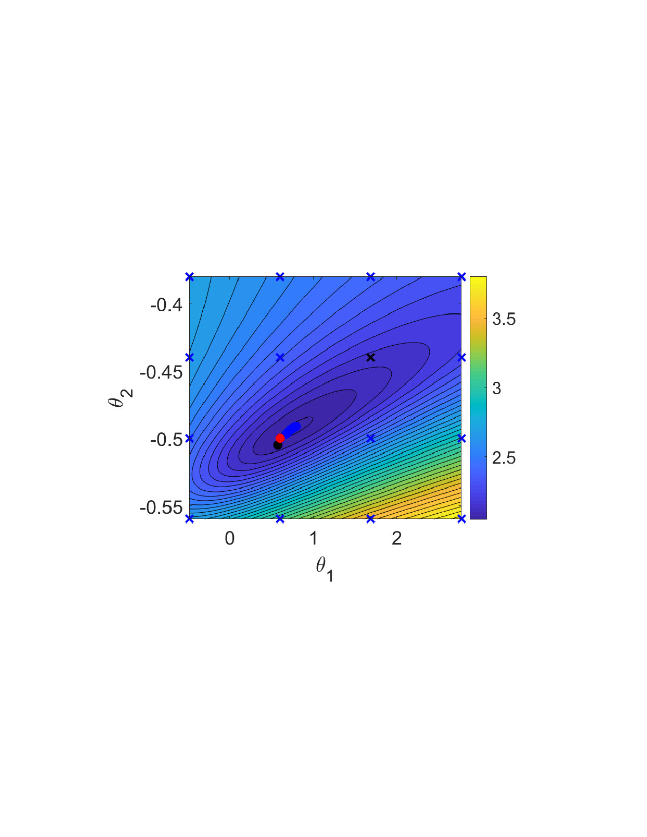 Figure 1
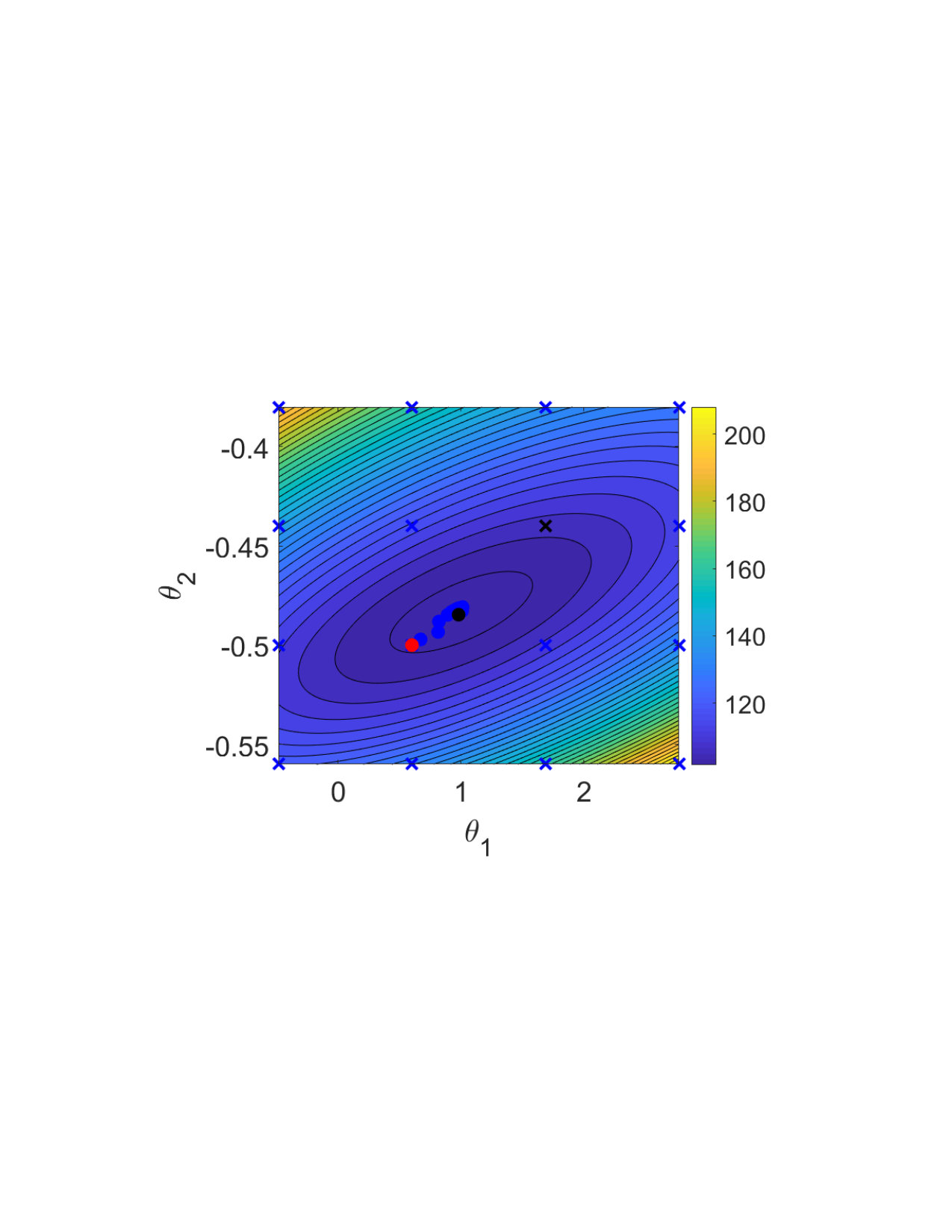 Figure 2
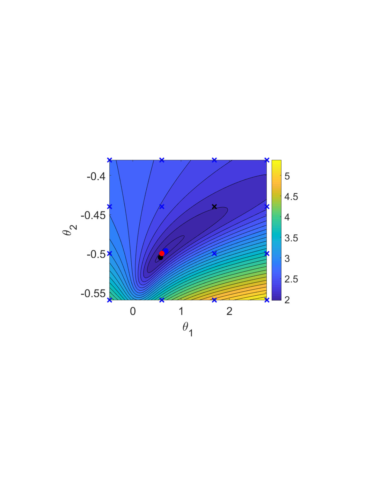 Figure 3
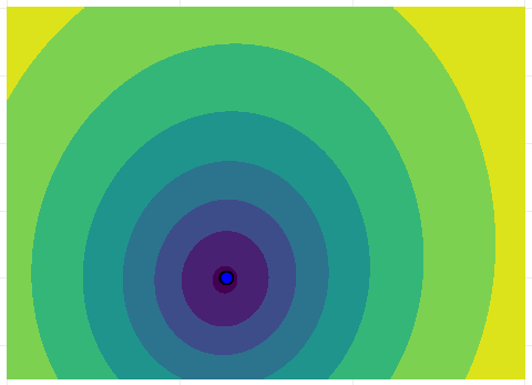 Figure 4
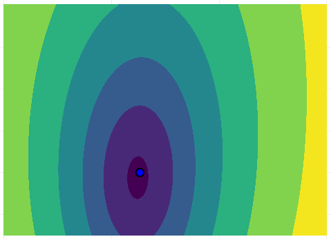 Figure 5
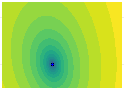 Figure 6
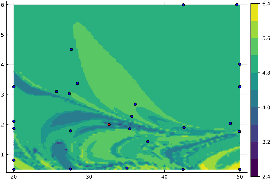 Figure 7
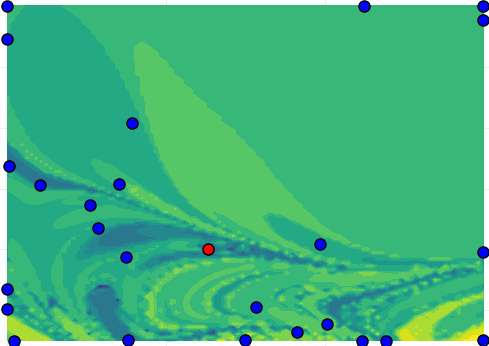 Figure 8
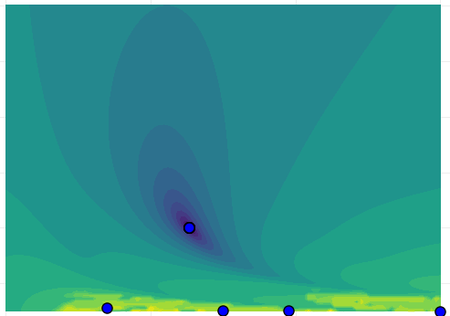 Figure 9
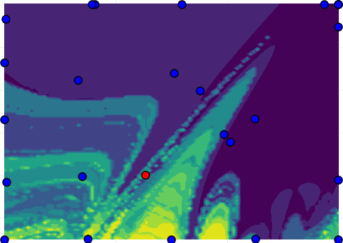 Figure 10
 Figure 11
 Figure 12
 Figure 13
 Figure 14
 Figure 15
 Figure 16
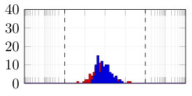 Figure 17
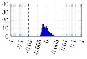 Figure 18
 Figure 19
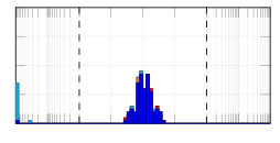 Figure 20
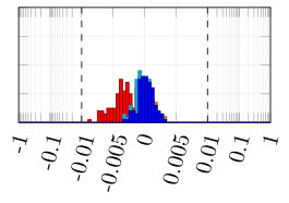 Figure 21
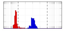 Figure 22
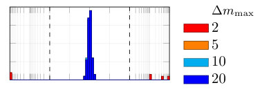 Figure 23
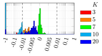 Figure 24
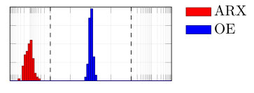 Figure 25
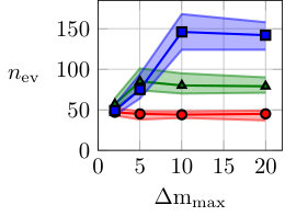 Figure 26
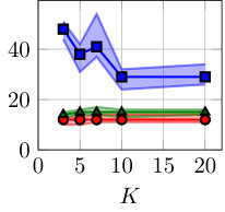 Figure 27
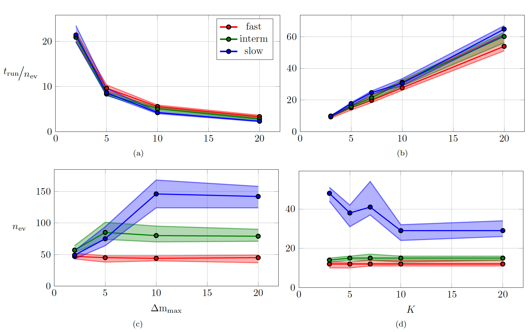 Figure 28
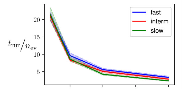 Figure 29
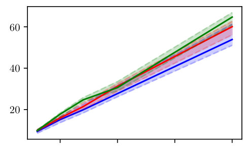 Figure 30
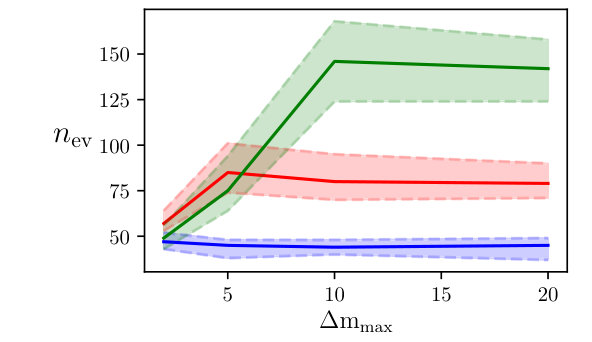 Figure 31
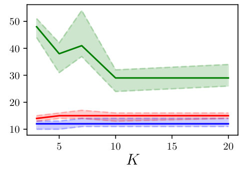 Figure 32
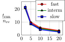 Figure 33
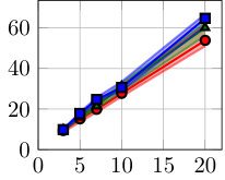 Figure 34
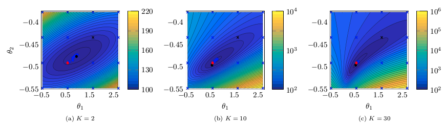 Figure 35
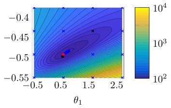 Figure 36
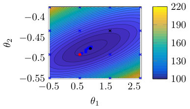 Figure 37
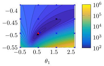 Figure 38
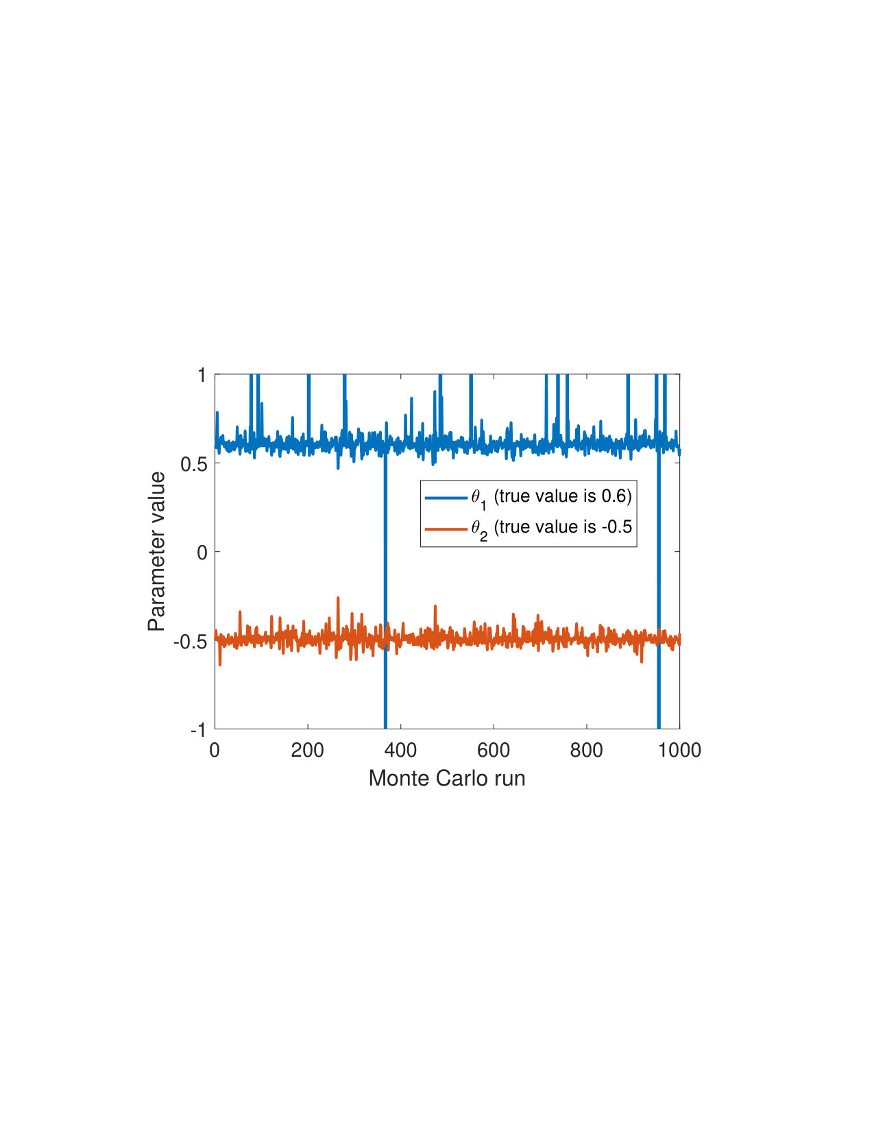 Figure 39
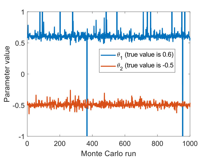 Figure 40
| function evaluations | run time (s) | |||||
| min | median | max | min | median | max | |
| 1 | 15 | 23 | 0.01 | 0.2 | 1.1 | |
| 43 | 1000* | 1000* | 0.7 | 24.7 | 27.3 | |
| 29 | 115 | 645 | 1.0 | 2.9 | 26.9 | |
| 21 | 50 | 65 | 1.7 | 2.9 | 3.8 | |
| multiple shoot. | MSA-PEM | |
|---|---|---|
| Problem dimension | ||
| # of constraints | ||
| Time-complexity (computing ) | ||
| Asymp. statistical properties | Independent of | Approach expected properties as |
| # of independent subproblems |
Peer Reviews
No public reviews on file for this paper yet. If you reviewed it on a platform where reviews are public (OpenReview, ICLR, NeurIPS, ICML), you can paste yours below so the community can read it here.
Code & Models
Videos
No videos yet. Explain this paper in a talk, walkthrough, or lecture? Add one.
On the smoothness of nonlinear system identification
Antônio H. Ribeiro [email protected]
Koen Tiels
Jack Umenberger
Thomas B. Schön
Luis A. Aguirre
Graduate Program in Electrical Engineering, Universidade Federal de Minas Gerais, Brazil
Dept. of Electronic Engineering, Universidade Federal de Minas Gerais, Brazil
Dept. of Information Technology, Uppsala University, Sweden
Dept. of Mechanical Engineering, Eindhoven University of Technology, The Netherlands
Abstract
We shed new light on the smoothness of optimization problems arising in prediction error parameter estimation of linear and nonlinear systems. We show that for regions of the parameter space where the model is not contractive, the Lipschitz constant and -smoothness of the objective function might blow up exponentially with the simulation length, making it hard to numerically find minima within those regions or, even, to escape from them. In addition to providing theoretical understanding of this problem, this paper also proposes the use of multiple shooting as a viable solution. The proposed method minimizes the error between a prediction model and the observed values. Rather than running the prediction model over the entire dataset, multiple shooting splits the data into smaller subsets and runs the prediction model over each subset, making the simulation length a design parameter and making it possible to solve problems that would be infeasible using a standard approach. The equivalence to the original problem is obtained by including constraints in the optimization. The new method is illustrated by estimating the parameters of nonlinear systems with chaotic or unstable behavior, as well as neural networks. We also present a comparative analysis of the proposed method with multi-step-ahead prediction error minimization.
keywords:
Prediction error methods, multiple shooting, system identification, output error models, parameter estimation.
, , , ,
1 Introduction
Prediction error methods [1] are a widespread class of methods for parameter estimation of dynamic models, which estimate the parameters by minimizing the error between predicted and measured trajectories. Many well-known estimation methods fit into this framework, such as minimizing the one-step-ahead prediction error or the free-run-simulation error. While the classical literature focuses primarily on the estimation of linear systems [1], the framework is general and enjoys appealing asymptotic properties for the general nonlinear setup [2].
Minimizing the one-step-ahead prediction usually yields an easier optimization problem, the minimization of the free-run simulation error or other recurrent structures, however, may produce more accurate models. These recurrent models often have a smaller generalization error [3], [4] and better capability when it comes to long-term prediction [5]. Minimizing recurrent structures is used, for instance, to improve the model structure selection of polynomial models [6], fine-tune parameters of nonlinear state-space [7] and block-oriented models [8].
It is common knowledge among practitioners that the optimization problem resulting from a recurrent model structure is harder to solve [9]. For linearly parametrized models and convex loss functions, minimization of one-step-ahead prediction error leads to a convex optimization problem; for recurrent model structures, the ensuing optimization is, in general, non-convex, complicating the search for global optima. Even during local optimization, recurrent model structures can lead to cost functions with poor smoothness properties, including many ‘jagged’ local minima, cf. Fig. 2(a) for an illustration. The current understanding of the relationship between model internal dynamics and the smoothness properties of the cost function is, however, imprecise and provides little insight into ways of circumventing the problem. Furthermore, the few studies that do investigate the objective function properties in this context are focused on linear systems, see e.g. [10].
The purpose of this paper is twofold. First, we aim to provide insight into the properties of the objective function arising in prediction error estimation problems in a general nonlinear setup. Specifically, we show how the smoothness of the objective function depends on two factors: the simulation length and the decay rate of the recurrent part of the prediction model. Second, we illustrate how this theoretical insight might be leveraged for the design and analysis of practical system identification methods.
The use of multiple shooting is analyzed in the context of prediction error minimization. This technique reformulates the optimization problem that arises from minimizing the difference between the output of a prediction model and the observed values. Rather than running the prediction model over the entire dataset, the multiple shooting formulation splits the dataset into smaller subsets and runs the prediction model over each subset. The equivalence with the original problem is obtained by including equality constraints in the optimization problem. This method results in a smoother objective function since it works with shorter simulations and prevents trajectories from diverging too much.
The multiple shooting formulation has reportedly provided improvements in the parameter estimation of ordinary differential equations [11], [12], [13] and in the solution of optimal control [14], [15], [16]. In the context of system identification, multiple shooting has been used for estimating polynomial nonlinear space-state models [17] and output error models [18] in settings where conventional methods fail to provide good solutions. Here, we extend this method to the entire class of prediction error methods. In addition, theoretical arguments are put forward to help understand why and when the proposed method is useful. We also present a comparative analysis with multi-step-ahead prediction error minimization [19], [20] [21], showing strengths and weaknesses of each method at a conceptual level and, also, with numerical examples.
2 Prediction error methods
While prediction error methods are widely known, they are often introduced from a linear perspective [1]. In the present section, this is accomplished in a nonlinear setting.
Consider the dataset containing measured inputs and outputs of a dynamical system. Prediction error methods assume an internal model that delivers output predictions , . A cost function is defined as the distance between predictions and measured values:
[TABLE]
The prediction model is, usually, parametrized by a parameter vector and, although such a dependence is not made explicit in the notation, depends upon . An estimate of the parameter vector may be obtained by minimizing .
Next we assume a dynamical, stochastic, discrete-time system as the data generating process. Let:
[TABLE]
where , are the maximum input and output lags. The examples we give next will differ in how they account for the noise in the model. But, in a noiseless situation, the data generating process for all of them corresponds to a difference equation . The parametrized function is defined and, if the noise assumption and model structure are correct, the minimization of the cost function would yield the estimate such that, as , then (or to a function with different structure but the same performance in predicting the training dataset). See Appendix D for a more precise description of the asymptotic properties of nonlinear prediction error methods.
Choosing the “true” model structure (one for which there exists a such that ) might be impossible in a practical application. Nevertheless the assumption is not so restrictive as it might appear, since there exist families of universal approximator functions (e.g. neural networks and polynomials) for which the distance might be made arbitrarily small within a compact set.
2.1 Nonlinear ARX models
The nonlinear ARX (autoregressive with exogenous input) model encodes an output that is corrupted by white process noise. That is, it assumes the data were generated by the stochastic discrete-time system:
[TABLE]
where is a zero-mean white noise. This assumption yields (cf. Appendix D) the prediction model:
[TABLE]
The minimization of the cost function in Eq. (1) for this prediction model yields an estimator with the desired asymptotic properties.
2.2 Nonlinear OE models
The OE (output error) model encodes an output that is corrupted by white measurement noise. That is, it is assumed that the data were generated by:
[TABLE]
where, again, is zero-mean white noise and represents the noiseless output. This assumption yields the following prediction model:
[TABLE]
Here represents an estimate of the noiseless output , which should approach the true value as .
2.3 Nonlinear ARMAX models
The nonlinear ARMAX (autoregressive moving average with exogenous input) model encodes an output that is corrupted by additive zero-mean process noise. In this case, the propagation equation allows the noise term to be propagated by the dynamics:
[TABLE]
This assumption allows the model to account for some forms of colored process noise and results in the following prediction model:
[TABLE]
Here represents an estimate of the noise corrupting the system and will approach the true noise if the estimated parameter vector approaches the true parameter value .
2.4 General nonlinear state-space framework
From now on, we will focus on a state-space representation that is general enough to encompass the prediction model from the above examples (for an appropriate choice of the functions and ). For this representation, the predicted output is given by:
[TABLE]
where denotes the internal state vector at instant . For the ARX model the transition state would be empty ; for the OE model ; and, for the ARMAX model .
Here . Using both inputs and autoregressive terms is what allows this state-space representation to encompass ARX, ARMAX and OE models, and also other representations such as the polynomial greybox models proposed in [22].
2.5 Initial conditions
In order to guarantee the desirable asymptotic properties, the prediction model needs to be simulated starting with the appropriate initial conditions . Since the true initial condition is unknown, there are two possible approaches when estimating the parameters.
The first approach is to fix , for some , and minimize the cost function (1). This approach is based on the idea that, for an asymptotically stable system, the influence of the initial conditions on the output will decrease over time for many cases of interest [23] and, hence, even if we can still obtain a good estimate of the parameters. In this case the first samples may be discarded, to make sure the transient errors are not too large. For the ARMAX model, an appropriate choice of initial values would be and, for the OE model, .
The second approach consists in including in the optimization problem, so it converges to and improves the quality of the parameter estimates. The optimization problem to be solved in this case is to minimize with both and as optimization variables:
[TABLE]
3 Smoothness of prediction error methods
The theorem below relates the Lipschitz constant of , and its gradient (i.e. -smoothness), to the simulation length . The Lipschitz constant of the cost function and the -smoothness both play a crucial role in optimization [24]. Lower values imply that local (Taylor) expansions of the cost function are more predictive of the cost function, and that the optimization algorithm can still converge while taking larger steps. It also gives an upper bound on how distinct in performance two close local minima may be.
The first part of the theorem below can be seen as a formalization of the exploding gradient problem, often studied in the context of neural networks [25]. The second part provides information about the explosion of second-order derivatives and curvature and it is, to the best of our knowledge, novel. As a result of the analysis, it is found that not only walls (resulting from large first-order derivatives) might be formed in non-contractive regions of the parameter space, but also regions with exploding curvature with multiple close local minima (cf. Fig. 2(a)). A recurrent neural network-oriented perspective of these results is discussed in a concurrent work from our group [26].
Theorem 1**.**
Let and in (6) be Lipschitz in with constants and on a compact and convex set . With and . If there exists at least one choice of for which there is an invariant set contained in , then, for trajectories and parameters confined within :
The cost function defined in (1) is Lipschitz with constant:111Where denotes the big O notation. It should be read as: if and only if there exist positive integers and such that .
[TABLE] 2. 2.
If the Jacobian matrices of h and g are also Lipschitz with respect to on , then the gradient of the cost function is also Lipschitz with constant:
[TABLE]
{pf}
See Appendix B.
For contractive models222We say that a dynamical system is contractive if, for all and , it satisfies , for ., under certain regularity conditions, we have and, according to the above theorem, both the Lipschitz constant and the -smoothness of the cost function can be bounded by a constant that, asymptotically, does not depend on the simulation length. All contractive systems have a unique fixed point inside the contractive region, and all trajectories converge to such a fixed point [27, Theorem 9.23]. Systems with richer nonlinear dynamic behaviors, such as limit cycles and chaotic attractors, and also unstable systems, are non-contractive and will always have . The Lipschitz constants and -smoothness for these systems may, according to Theorem 1, blow up exponentially (or polynomially for some limit cases) with the maximum simulation length.
Less formally, for models that have infinitely long dependencies (i.e. are non-contractive) the distance between trajectories of models that are close in the parameter space might become progressively larger along the simulation length because errors will accumulate. This might yield very intricate objective functions in some parts of the parameter space and make the optimization problem very dependent on the initial estimate.
4 Multiple shooting
The theoretical results from the previous section suggest that long simulation lengths might yield regions of the parameter space where the cost function is intricate, hence hard for the optimization algorithm to navigate.
In this section, we propose the application, in the context of prediction error methods, of a technique called multiple shooting for which the maximum simulation length is a design parameter. This enables solving problems that would be impossible or very hard to solve in the setting of Section 2, which will be named single shooting from now on.
4.1 Method formulation
For the multiple shooting formulation, rather than simulating the prediction model (6) through the entire dataset from a single initial condition vector , the data is split into intervals , , each one with its own set of initial conditions . The -th vector of initial conditions is used to compute over :
[TABLE]
Since the length of the simulation is limited to the shorter interval , the trajectory is less likely to strongly diverge and this typically helps the optimization procedure by making the objective function smoother.
Let , we define:
[TABLE]
to be the cost function associated with the -th interval, where the prediction depends upon and , according to (10). The multiple shooting formulation makes use of the following objective function:
[TABLE]
This objective function includes states as free variables in the optimization. Hence, rather than reinforcing the cohesion of the states by defining them through a recurrence relation that casts a dependency of all the way back to the initial condition , as in the single shooting formulation, the cohesion between subsequent states is achieved through optimization constraints, resulting in the following problem:
[TABLE]
The next theorem provides the equivalence between (7) and (12). The theorem and its corollary are a formalization of the intuition provided in Fig. 1 and they give further insight into how the constraints in the multiple shooting formulation are used to imitate a single simulation throughout the entire dataset.
Theorem 2**.**
If and , then .
{pf}
Let us call , and , the states and predictions in, respectively, the single shooting simulation and in the -th multiple shooting interval. For a fixed , if then for all . Hence, inside this same interval, . Applying this for every it follows from the respective definitions that: .
Corollary 3**.**
The pair is a global solution of (7) if and only if there exist such that is a global solution of the optimization problem (13).
Multiple shooting can be understood as a generalization of the single shooting case. That is because, if and , both methods result in the same optimization problem. Multiple shooting, however, might provide some advantages. The method is more amenable to parallelization, since each cost function and its associated derivatives can be computed independently and, possibly, in parallel. Also, long simulations usually yield larger numerical errors due to finite precision errors that accumulate along the simulation, hence multiple shooting shorter simulation intervals also attenuate this problem. Finally, multiple shooting cost function has better smoothness properties that will be investigated next.
4.2 Properties of the cost function
For the multiple shooting method, the Lipschitz constant of and of its gradient, and depend asymptotically on rather than on (See Appendix C). For instance, if :
[TABLE]
Since is a design parameter, it is possible to have some control over the Lipschitzness and -smoothness of the objective function in the non-contractive region of the parameter space ().
5 Implementation and numerical examples
In this section, numerical examples are presented. The cost function smoothness is investigated through the lens of the theoretical results in Section 3 and it is shown how multiple-shooting might help mitigate some problems.
The equality-constrained problem (12), which arises from the multiple shooting formulation, is solved using an implementation of the sequential quadratic programming solver originally described in [28] available in the SciPy library [29]333 scipy.optimize.minimize(method=‘trust-constr’). The procedure used for computing the derivatives is explained in Appendix A. Additional numerical examples are provided in Appendix F.
5.1 OE model for a chaotic system
This example illustrates how multiple shooting makes prediction error methods more robust w.r.t. the choice of initial conditions for the optimization. A dataset with samples is generated using the logistic map [30]:
[TABLE]
with . From the generated dataset we try to estimate an output error model with the same structure.
Fig. 2(a) illustrates the objective function for the single shooting case. The data generating system, Eq. (15), presents chaotic behavior for , which explains the very intricate objective function in this region. For chaotic systems, small variations in the parameters may cause large variations in the system trajectory and, consequently, abrupt changes in the free-run simulation error. This explains why the cost function used in estimating an OE model has many local minima for this problem.
The solutions found by the solver, for different initial guesses, are also displayed in Fig. 2(a). Notice that the solver fails to find the true solution because it always gets trapped in local stationary points near the initial guess. Even in this noiseless scenario, the estimation problem is very challenging due to the chaotic nature of the system. Hence, for a simulation that is sufficiently long, the trajectories will differ significantly even for small parameter variations.
Multiple shooting makes the problem easier by limiting the maximum simulation length. Fig. 2 (b), (c) and (d) display the objective function and the solutions found by the solver starting from different initial guesses. The estimation procedure becomes easier as is made smaller. For Fig. 2(c) the solver already converges to the true parameter for some initial guesses, but not for all of them. For Fig. 2(d), the solver converges to the true solution for all initial guesses that have been tested.
For the multiple shooting case, besides , the initial conditions are also optimization parameters. To help with the visualization of this multidimensional problem, Fig. 2(b), (c) and (d) display the main curve corresponding to the objective function for the true initial conditions and faded lines corresponding to the objective function for perturbed initial conditions. Another consequence of the problem having more parameters than displayed in the figure is that the cost function found by the solver does not need to lie on any of the objective function curves displayed in the figure, since it may have a different set of initial conditions .
It is important to highlight that the mechanism used here is not to take the system outside of the chaotic regime, but rather avoid simulating the system for too long. By doing that, we avoid the major problem that arises in the identification of chaotic systems, i.e. the high sensitivity to parameters and initial conditions. This results in a better behaved objective function (cf. Fig. 2). The constraints allow the equivalence with the original prediction error problem (according to Theorem 2 and Corollary 3).
Table 1 gives the number of function evaluations and the running time for the four situations displayed in Fig. 2. The convergence happens within just a few iterations for (single shooting) because any initial point is probably very close to some optimal local solution. As we reduce the objective function becomes less intricate and this is reflected in the convergence of the solver. For the solver takes much longer to converge. We believe this happens because the local solution is not so close in the parameter space to the initial guess anymore. As is further decreased, however, the convergence becomes faster because it is dealing with, what is believed to be, a smoother problem that can be handled more accurately by low order approximations.
5.2 Pendulum and inverted pendulum
Consider the following discrete-time nonlinear system:
[TABLE]
which corresponds to a pendulum model, discretized using the Euler approximation , where is the gravity acceleration, is the mass connected to the extremity of the pendulum, is the length of the (massless) rod connecting the mass to the pivot point, and is the linear friction constant. It has two states: the angle of the mass () and the angular velocity (). The input is the force applied to the mass.
This system has multiple equilibrium points, namely, for . The equilibrium points at are stable and the equilibrium points at are unstable. For this system, with , , , and , we define three different datasets: (a) A dataset for which small inputs are applied to the system, that stays under the influence of the stable point and stays, approximately, inside the range ; (b) A dataset for which the system is maintained close to the unstable point by a linear controller; and, (c) A dataset for which the input is large enough to drive the pendulum to full rotations around its center. The output corresponding to those three situations are displayed in Fig. 3.
Fixing and parameters and of an output error model with the structure presented in (19) were estimated from the data. A visualization of the cost function is presented in Fig. 4 together with numerical solutions found by means of the single shooting and multiple shooting formulation starting from different initial conditions.
For dataset (a), the single shooting formulation is able to recover the true parameters from data for most of the initial conditions. Some exceptions occur when initialized far away from the correct initial conditions. For datasets (b) and (c), for which the system needs, respectively, to operate close to the unstable dynamics or to account for the existence of multiple fixed points, the cost function is highly intricate and full of local minima. In this case, the optimization algorithm, even when initialized close to the local solution, fails to converge to reasonable solutions. This result is consistent with Theorem 1 and how the smoothness of the objective function degenerates (exponentially) on sets of the parameter space for which the prediction model is non-contractive, such as the trajectories close to the unstable fixed point of the system (19). The use of multiple shooting yields an objective function that looks similar to a paraboloid in the region of interest for the three cases and the optimization procedure converges to the true parameter regardless of the initialization.
For nonlinear ARX, ARMAX or OE models the states are directly measured (possibly with some noise contamination) and the initialization of the optimization parameters follows naturally from the considerations in Section 2.5. Here, however, the state variable is not measured. This variable can be interpreted as the derivative of , so a finite difference approximation was used in the initialization of the intermediary initial conditions . Although the high-pass behavior of the derivative amplifies the noise, this choice was still better than a completely arbitrary one.
6 Comparison with multi-step-ahead prediction error minimization
6.1 Multi-step-ahead prediction error minimization
Multiple-shooting is presented here as a possible way of limiting the simulation interval . A method that appears in the system identification literature that also has a similar effect is the multi-step-ahead prediction error minimization (MSA-PEM) [19], [20] [21]. The approach fits well into the moving horizon framework [20] and is popular for system identification in model predictive control application. The method has been studied primarily in a linear model setting, nevertheless it can be extended to a nonlinear setting [21].
In the MSA-PEM estimation, the simulation is truncated to a fixed number of steps backwards. That is, for each , we define an auxiliary variable and an initial condition . Starting from the system is propagated using the state equation: to simulate the evolution of this auxiliary state variable for . The prediction is then computed using . The parameters are obtained by minimizing a cost function similar to (1).
Multiple shooting is equivalent, in the sense of Theorem 2 and Corollary 3, to solving the original (single shooting) problem regardless of the choice of simulation interval . MSA-PEM, on the other hand, is equivalent to the original formulation only if . The next example illustrates how the statistical properties of the method change as varies from to .
6.2 Example: estimating the output error model for second-order under-damped system
A dataset with samples is generated using the equation:
[TABLE]
Here represents the noiseless output, and represents the white output noise that is introduced during the data generation. At each , is a Gaussian random variable with standard deviation .
Let denote the parameter vector used for the data generation. Three different settings are considered: (a) ; (b) ; and, (c) . The three settings correspond to underdamped linear systems with different response-times: in (a) the system responds fast to input changes and has a time constant ; in (c), it responds slowly and ; and, (b) is an intermediate setting with .
From the synthetically generated data, the parameters of a model with the same structure are estimated. The experiment is repeated 100 times, each time corresponding to a different realization (i.e., different random seed) of the data generation. The result of the Monte Carlo procedure is displayed in Fig. 5 for the parameter estimation using ARX, standard (single shooting) output error, multiple shooting, and MSA-PEM. We show the difference between estimated and true values for the first parameter, . Similar results have been obtained for and .
Due to the presence of white output error, using output error estimation yields consistent and well-behaved results. ARX estimation, on the other hand, is biased, and its histogram is not centered around zero. This is more evident either in 5(b) or in 5(c). In Fig. 5(a), which correspond to the fast response system, there is not much difference between the two estimation procedures, mostly because any disturbance fade away very quickly, yielding similar statistical properties for the two estimators.
Multiple shooting estimation results are similar to the (single shooting) output error estimation. For some choices of , the optimization problem might actually be made harder due to the increase in the problem dimension. In this case, the algorithm seems to fail a few times, which can be observed in the histogram as a few outliers in the estimated parameter distribution. Except for these outliers, all the different choices of yield very similar distributions for the estimated parameters.
For MSA-PEM, the estimation results vary qualitatively among the three settings. For the intermediate setting, midway qualitative behavior between ARX and output error estimation is obtained, approaching that of output error estimation as increases. For the fast-response system, a similar interpretation is possible, however, there is not much difference between using ARX and output error estimation to begin with (cf. Fig 5 (a)), hence all -step-ahead choices yield similar results. Finally, for the slow-response setting, minimizing the multi-step-ahead prediction error does not offer a direct compromise between ARX and output error estimation and, for or , it is possible to observe a bimodal distribution with one peak distant from zero. And yields the best results.
In Fig. 6, the computational cost of multiple shooting and MSA-PEM are compared. The average running time divided by the number of function evaluations is displayed in Fig. 6(a) and (b). This accounts for the computational cost of computing the cost function, derivatives, and performing the matrix factorizations needed by the optimization algorithm at each iteration. Figure 6(c) and (d) display the number of cost function evaluations needed for the optimization algorithm to converge. The next section studies time and memory complexity of the methods and explains the obtained results in a more general context.
6.3 Computational cost
As observed in Fig. 6(b), MSA-PEM has an average running time per iteration that grows linearly with the number of stages. Since the problem dimension and the factorization cost per iteration remain constant, it is the time complexity of computing the cost function (and its derivatives) that accounts for the linear growth. In Appendix E, we discuss in detail the computation of and arrive at the time complexity of .
Multiple shooting estimation, on the other hand, has an average running time per iteration that decreases with the maximum simulation length . This is displayed in Fig. 6(a). In this case, the cost of computing is and does not depend on the simulation length. The increase in the problem dimension, however, yields more costly factorizations (cf. Appendix A), which results in the increased computational cost per iteration.
For multiple shooting, shorter simulation lengths allow the solver to converge with fewer function evaluations. This is in agreement with the theory presented in this paper, which suggests longer simulation lengths might result in poor smoothness properties and make the optimization problem harder to solve. Applying the same reasoning to MSA-PEM, it is natural to expect that smaller values of would yield convergence with fewer iterations. This, however, does not seem to be the case for the slow time-response setting, maybe because MSA-PEM often converges to the wrong parameters in this setting (as shown in Fig. 5(i)).
In general, the number of function evaluations for MSA-PEM is lower than for multiple shooting because the resulting problem is unconstrained, rather than constrained, for which more efficient procedures are available.
Finally, MSA-PEM and multiple shooting are both amenable to parallelization, even though this is not explored in the examples. During MSA-PEM implementation, it is possible to instantiate different processes (or threads) for computing each prediction (and the corresponding derivatives) in parallel. Multiple shooting, on the other hand, subdivides the problem into independent subproblems.
6.4 Cost function smoothness and estimation tradeoffs
Both MSA-PEM and multiple shooting allow the user to control the maximum simulation length, hence the smoothness of the cost function (cf. Section 3), by setting for the MSA-PEM and for the multiple shooting. These parameters, however, affect diverse aspects of the estimation problem, which are summarized in Table 2. Multiple shooting has an exact equivalence with the original single shooting problem regardless of the simulation length and the parameter offers a tradeoff between the problem dimension and smoothness properties of the cost function. MSA-PEM keeps the problem dimension fixed, and, as increases, it is possible to approach the behavior of methods with distinct statistical properties (not always in a smooth way, as shown in Fig. 5(i)), at the expense of an increased computational cost and worse smoothness properties.
Some refinements are proposed in the literature. For instance, [19] propose to average over different values of , to obtain a slower but smoother convergence to output error estimation as . In [21], on the other hand, the method starts from the one-step-ahead prediction solution and increases by one in each iteration until convergence. We give an numerical example using such approach in Appendix F.
7 Conclusion
The relevance of this paper lies in the rather general setting for which the proposed methods and results hold. The main technical contribution is to show that for dynamic prediction models that are non-contractive (i.e. do not converge asymptotically to a single stable point) in the region of interest, the upper bound for the Lipschitz constant and the -smoothness blows up exponentially with the simulation length, and this can make the optimization problem very hard to solve. This was illustrated using numerical examples with systems that are non-contractive due to the presence of chaotic regions and unstable equilibrium points. Because of these regimes, the objective function becomes very intricate in some regions of the parameter space and the optimization algorithm fails to find a good solution. Even for problems that are contractive in the region of interest, multiple shooting might help in preventing the solver from getting stuck in undesirable regions of the parameter space, hence facilitating the convergence to a good solution (cf. Section 5.2).
Multiple shooting makes the simulation length a design parameter and hence allows solving optimization problems that would be infeasible in a single shooting setting. The price paid compared to single shooting methods is that a nonlinear constrained optimization problem must be solved instead of an unconstrained one. It also makes it harder to generalize to situations other than batch training, such as online training. MSA-PEM is another approach that allows some control over the smoothness of the cost function, but with different tradeoffs (see Table 2) between smoothness, asymptotical properties and computational cost to be taken into consideration.
Appendix A Computing the derivatives
A.1 Sensitivity equations
Let the Jacobian matrices of with respect to and to evaluated at the point be denoted, respectively, as and . Similarly, the Jacobian matrices of are denoted as and . Also, we denote the Jacobian matrices of with respect to and to as and . And the Jacobian matrices of are denoted as and .
A direct application of the chain rule to (6) gives a recursive formula for computing the derivatives of the predicted output in relation to the parameters in the interval :
[TABLE]
A similar recursive formula may be used for computing the derivatives of the predicted output in relation to the initial conditions:
[TABLE]
Finally, we define and
.
A.2 Single shooting
For the cost function defined as in (1), its gradient is given by:
[TABLE]
Its Hessian is given by:
[TABLE]
where . Ignoring is a common approximation used in least-squares algorithms, that will also be used here when computing derivatives numerically.
A.3 Multiple shooting
In order to solve the problem using the sequential quadratic programming solver [28] we must be able to compute: i) The cost function ; ii) its gradient ; iii) the constraints; iv) the Jacobian matrix of the constraints (which can be represented using a sparse representation); and, v) for any given vector , the product of the Lagrangian444The Lagrangian is given by: . Hessian and the vector (the full Lagrangian Hessian matrix does not need to be computed). The following sequence provides a way of computing all derivatives required by the optimizer.
Algorithm 1** (Derivatives).**
For a given parameter and set of initial conditions:
For , do:
- (a)
For :
- i.
Compute and with (6). 2. ii.
Compute , , and . 3. iii.
Compute and with the sensitivity equations. 2. (b)
Compute using Eq. (11). 3. (c)
Compute using a formula equivalent to (23). 4. (d)
Approximate the product of the Hessian with a given vector, , using the first terms from a expression equivalent to (24) 2. 2.
Compute with (12); 3. 3.
Compute ; 4. 4.
Compute the value of the constraint from the values of , ; 5. 5.
Compute the Jacobian matrix of the constraints from , ; 6. 6.
Compute ; 7. 7.
Compute the product of the Hessian with a vector using 2-point finite differences; 8. 8.
Compute the product of the Lagrangian Hessian and a vector , summing the Hessians computed in steps 6 and 7.
Some approximations were used for computing the second derivatives:
- for computing the Hessian of the objective function, the standard least-squares approximation for the Hessian is used; and, 2) for computing the Hessian of the constraint we use finite-difference approximation. The use of finite differences here comes inexpensively because we only need to evaluate the Hessian times a vector, and not the full matrix. Hence, it can be done at the cost of an extra Jacobian matrix evaluation.
Notice that step (1) from the above algorithm can be parallelized, with different processes (or threads) performing the computation for different values of .
Appendix B Proofs
B.1 Preliminary results
Lemma 4**.**
Let and be two Lipschitz functions on with Lipschitz constants and . Then,
- a)
* is also a Lipschitz function on with the (best) Lipschitz constant upper bounded by ;* 2. b)
if, additionally, and are bounded by and on , then is also a Lipschitz function on with the (best) Lipschitz constant upper bounded by .
B.2 Proof of Theorem 1 (a)
Assume two different trajectories resulting from simulating the system (6) with parameters and initial conditions and , respectively. We denote the corresponding trajectories by and . Let us call:
[TABLE]
Because h and g are Lipschitz in we have:
[TABLE]
for all and in . Applying these relations recursively we get that:
[TABLE]
Since is positive, the constant multiplying the second term in the above equation is always larger than the constant multiplying the first one. Hence, taking the square root on both sides of the above inequality and after simple manipulations, we get:
[TABLE]
where:
[TABLE]
Since is compact and is a (Lipschitz) continuous function of the parameters and initial conditions, then is bounded in , i.e. . And, it follows from (26) and from the existence of an invariant set555There are multiple ways to guarantee the invariant set premise will hold, but a very simple way is to just choose h such that . In this case, is an invariant set and if contain this point the premise is satisfied. For this specific case, one can just choose and it follows from (26) that . The more general case, for any invariant set, follows from a similar deduction. in that .
The following inequality follows from (1):
[TABLE]
where . And, by putting together (28) and (26):
[TABLE]
for . The asymptotic analysis of this expression with regard to yields (8).
B.3 Proof of Theorem 1 (b)
It follows from (23) that:
[TABLE]
where we have used the notation to denote the difference between evaluated at and . Analogously, denote the difference between evaluated at the two distinct points.
From equation (21) and (22) it follows that:
[TABLE]
Since, the Jacobian of h is Lipschitz with Lipschitz constant , it follows that:
[TABLE]
Using a procedure analogous to the one used to get Eq. (26), it follows that:
[TABLE]
where is defined as in (27). An identical formula holds for and a similar formula, replacing with , holds for and .
Since h and g are Lipschitz with Lipschitz constants and it follows that , , and . Hence, it follows from (26), (30), (32) and the repetitive application of Lemma 4 that , , and are upper bounded by multiplied by the following constants:
[TABLE]
where and:
[TABLE]
Hence,
[TABLE]
where
[TABLE]
Putting everything together the asymptotic analysis of results in (9).
Appendix C Lipschitz analysis for the multiple shooting
The next theorem follows from basic inequality manipulation and relates the Lipschitzness and -smoothness of the cost function with that of its components .
Theorem 5**.**
Defining as in (12), if each component is Lipschitz continuous with constant then is also Lipschitz with constant equal to or smaller than . Additionally, if the gradient of each component is Lipschitz continuous with constant then is also Lipschitz with constant equal to or smaller than .
{pf}
For and we have that:
[TABLE]
where . And similarly, , which yields the second result.
Appendix D Asymptotic properties of prediction error methods
D.1 Notation and data generation process
Consider and to be one realization of the random variables and . And denote:
[TABLE]
Hence, rewriting the data generation difference equations for nonlinear ARX, output error and ARMAX (see Sections 2.1, 2.2 and 2.3) with the random variables yield, respectively:
[TABLE]
Here is a random variable representing the noise that is injected in the system. Notice that there is a deterministic additive relation between and . Hence, if and are determined, so is , or, conversely, if and are determined, so is .
D.2 Optimal output prediction
Let us define the optimal output prediction at time as the following conditional expectation:
[TABLE]
which is, in the least square sense, the best prediction for the output given its previous values.666 This prediction provides the smallest squared conditional expected error between the predicted and observed values: \hat{\mathbf{y}}_{*}[k]=\arg_{\hat{\mathbf{Y}}}\min E\left\{\|\mathbf{Y}[k]-\hat{\mathbf{Y}}\|^{2}~{}\Big{|}~{}\underline{\mathbf{u}}[k],\underline{\mathbf{y}}[k-1]\right\}.
For the nonlinear ARX, output error and ARMAX models the optimal output predictions are given, respectively, by:
[TABLE]
which follows from a direct application of the definition (33) to the stochastic difference equations that are assumed for the data generation in each case.
D.3 Ideal cost function
Ideally, the model predicted output should be as close as possible to the optimal one . The distance between the two series is quantified by the cost function:
[TABLE]
Now, back to the examples, given a parametrized function with the correct model structure (that is: there exist such that ), it follows from Eqs. (3), (4) and (5) that yields , and hence is a minimizer of .
D.4 Uniform convergence of
The optimal cost function is not available for optimization. Nevertheless, under some mild regularity conditions, it has been proved that in probability as and that this convergence is uniform [2].
If has a single minimum and is convex in a convex set containing the minimizer of converges to the minimizer of [31, Theorem 2.1]. Alternative conditions for this to hold are given in [2]. For our three examples, this would imply (convergence in probability for ). If the conditions are not satisfied, the uniform convergence, at least, guarantees that the minimizer has an equivalent performance (as ). Additionally, in [32] it is shown that if the solution is unique the estimator has an asymptotic normal distribution.
Appendix E Computational cost of MSA-PEM
As mentioned in Section 6.3, the computation of the cost function (and its derivatives) for the MSA-PEM method has linear time complexity with . The rate at which the time complexity grows, however, depends on implementation choices. We use the model estimation described in the experiment in Section 6.2 to explain the tradeoffs of those choices. Propagating steps-ahead the linear system can be performed in two ways. The first is to introduce intermediate variables:
[TABLE]
The other is to simplify the computation in advance, resulting in a system of higher order:
[TABLE]
where the coefficients depend on (for instance ) and are computed in advance. For the first approach, computing the cost function has time-complexity ; for the second, the computational cost is slightly smaller: . The reduced computational cost is obtained because some computations are performed in advance and stored. Hence, the additional time-efficiency comes at the cost of storing the computation in advance, and the memory of the first method is , while in the second approach the memory complexity is .
For linear systems, it is easy to find the optimal simplified computation in advance by using Diophantine equations [19]. In the experiment in Section 6.2, however, we use the less time-efficient approach. The general tone of our discussion justifies this choice since this implementation can easily be applied to generic systems. And, while heuristic solutions might be employed to simplify the computations in advance, there is no general approach for all types of nonlinear systems. Regardless of this design choice, however, the observed linear growth of the computational cost with is expected.
Appendix F Additional experiments
F.1 Neural network for modeling pilot plant
This example makes use of data from the level process station described in Example 1 from [3]. As in the original paper, we use a neural network to model the water column height as a function of the voltage applied to a control valve that modulates the water flow. We compare three different training methods: i) minimizing the one-step-ahead prediction error (NN ARX) ii) minimizing the free-run simulation error using single shooting method (NN OE - SS); and, iii) minimizing the free-run simulation error using multiple shooting method (NN OE - MS).
The neural network (NN) training depends on the weight initialization, hence the performance of the neural network can be regarded as a random variable and is displayed in Fig. 7, which compares the empirical cumulative distribution of the mean square error (MSE) over the validation dataset for the three methods. A linear ARX model ( and ) was trained and tested under the same conditions to serve as the baseline. Methods (i) and (ii) and the linear ARX baseline were described in [3]. Method (iii) is introduced in this paper.
The cumulative distribution function gives, for each -axis value, the probability of the method to yield a validation MSE smaller than or equal to this value. It was estimated from 100 realizations of the neural network training procedure. Fig. 7 shows that for more than 90% of the realizations, estimating the parameters by minimizing the free-run simulation (NN OE) offers significant advantages over the minimization of the one-step-ahead error (NN ARX). When using a standard single shooting formulation, however, it also makes the parameter estimation procedure more sensitive to the initial conditions, with the algorithm yielding some really bad results for some initial choices [3]. This results in a long-tailed distribution for the MSE (Fig. 7). More precisely, in 10 out of 100 realizations the NN OE - SS model yields a performance that is inferior to the linear ARX baseline, some of the realizations worse than the linear baseline by a factor of 100. The performance of the NN OE - SS and NN OE - MS is very similar for 90% of the realizations, the tail of the distribution, however, is very different, with the multiple shooting procedure rarely producing very bad results. In order to highlight the differences, results where NN OE - SS and NN OE - MS are worse than the baseline are presented, respectively, as blue and red circles in Fig. 7.
This example illustrates how the use of multiple shooting alleviates the problem of high sensitivity to initial conditions, making it possible to estimate output error models with extra robustness against variations of the initial conditions and lower probability of getting trapped at local minima with very bad performance.
This example also shows the limitations of the multiple shooting formulation. The training time for NN OE - MS model is 282 seconds, for NN OE - SS model is 3.9 seconds, and for NN ARX model is 3.3 seconds. This means that the single shooting parameter estimation could be repeated, roughly, 70 times for each multiple shooting run. Hence solving the single shooting problem several times and choosing the best result would also avoid very bad solutions and could, still, be computationally less expensive than solving the multiple shooting problem. The longer training time is due to two factors: i) per iteration the multiple shooting approach takes, roughly, 3.5 times more than the single shooting approach; and, ii) it takes, approximately, 20 times more iterations to converge. Both are consequences of the fact that a higher dimensional constrained optimization problem is being solved.
F.2 Incremental initialization approach for the MSA-PEM
Here, we revisit the setup of the first numerical example presented in [21]. A dataset with samples is generated using the equation:
[TABLE]
The data generator parameters are and , represents the noiseless output and the white output noise. The input is generated by the following AR process:
[TABLE]
where is white Gaussian noise with variance one. The output noise has variance , where is the output variance.
A model with the same structure as the data generator is estimated using MSA-PEM. Fig. 8 displays the cost function and the result of parameter estimation for several initial optimization conditions. Besides the results of the vanilla implementation, in blue, we also show, in black, the refinement proposed in [21]. For this refinement, the prediction starts from the one-step-ahead solution, and in each iteration increases by one. That is, the MSA-PEM problem is initialized from the (partial) solution of the MSA-PEM estimation. The intermediary results for the refined implementation are displayed in the plot. With the algorithm being iterated up to the -th iteration.
The effect of increasing the simulation length can be observed in this example, with a larger yielding less smooth cost functions. The refinement proposed in [21] allows the estimation to approach the desired asymptotic statistical properties while optimizing more complicated cost functions progressively. The results in Fig 8, show this refinement yield improvements over the vanilla implementation, maybe because it avoids optimizing the harder optimization problems from a distant initial estimate.
Appendix G Equality-constrained optimization solver
This appendix describes the implementation of the solver described in [28], which is used in the numerical examples. The method is able to solve large-scale equality-constrained optimization problems:
[TABLE]
where : and : are twice continuously differentiable functions.
The algorithm solves a sequence of Taylor approximations in order to gradually converge towards a local solution of (37). At the -th iteration, the algorithm builds a local model around the current iterate , computes the update by solving a quadratic programming problem and then updates the solution:
[TABLE]
The algorithm is a trust-region method [33], in the sense that the update must respect , for which is known as trust radius and should reflect the trust the algorithm has on the local approximation of the cost function. If the current local approximation is not a good one, the method does not allow a very large step to be taken.
G.1 Quadratic programming subproblem
At each iteration, in order to compute the step update , the method solves the trust-region quadratic programming (QP) sub-problem:
[TABLE]
where is the current iterate, is the current approximation of Lagrange multipliers, is the gradient of and is the Jacobian matrix of . As in Appendix A, denotes the Lagrangian:
[TABLE]
and is the Hessian in relation to the variable .
The current approximation of the Lagrange multipliers is obtained by solving the least-squares problem:
[TABLE]
The vector is included in the problem in order to guarantee linear and trust-region constraints are always compatible. is defined as for a value of satisfying:
[TABLE]
for (in our implementation ). For this choice of the linear constraints are always compatible with trust-region constraints.
The sub-steps are solved in rather economical fashion using efficient methods to get an inexact solution to each of the sub-problems. The QP problem (39) is solved using a variation of the dogleg procedure (described in [34], p.886) and (42) is solved using the projected conjugate gradient (CG) algorithm [35].
G.2 Implementation details
Here we define the merit function, , which combines the constraints and the objective function into a single number that can be used to compare two points and to reject or accept a given step. It is given by:
[TABLE]
where the penalty parameter is updated through the iterations. This parameter must increase monotonically for the algorithm to converge. Some additional guidelines are provided in [34], p.891.
The selection of the trust radius and the step rejection mechanism are based on the ratio:
[TABLE]
between the reduction of the merit function and the reduction predicted by the local (Taylor approximation) model:
[TABLE]
The ratio measures the agreement between the observed and expected reduction and is used as decision variable when accepting or rejecting the update and enlarging or reducing the trust radius .
G.3 Algorithm Overview
The full algorithm is summarized next.
Algorithm 2** (Trust-region sequential QP solver).**
*At each iteration, until some stop criterion is met (e.g.
), repeat:*
Compute , , and ; 2. 2.
Compute least squares Lagrange multipliers ; 3. 3.
Compute ; 4. 4.
Apply dogleg method in order to compute and (such that the resulting problem is feasible); 5. 5.
Compute using the projected CG method; 6. 6.
Choose penalty parameter ; 7. 7.
Compute reduction ratio ; 8. 8.
Accept or reject step using as decision variable; 9. 9.
Enlarge or reduce trust-radius using as decision variable.
Code avaibility
The code for reproducing the examples is available in: github.com/antonior92/MultipleShootingPEM.jl.
Acknowledgements
This work has been supported by the Brazilian agencies CAPES - Coordenacão de Aperfeiçoamento de Pessoal de Nível Superior (Finance Code: 001), CNPq - Conselho Nacional de Desenvolvimento Científico e Tecnológico (contract number: 303412/2019-4, 200931/2018-0 and 142211/2018-4) and FAPEMIG - Fundação de Amparo à Pesquisa do Estado de Minas Gerais (contract number: TEC 1217/98), by the Swedish Research Council (VR) via the projects NewLEADS – New Directions in Learning Dynamical Systems (contract number: 621-2016-06079) and Learning flexible models for nonlinear dynamics (contract number: 2017-03807), and by the Swedish Foundation for Strategic Research (SSF) via the project ASSEMBLE (contract number: RIT15-0012).
The reference list from the paper itself. Each links out to its DOI / PubMed record.
- 1[1] L. Ljung, System Identification: Theory for the User . Prentice Hall, second ed., 1999.
- 2[2] L. Ljung, “Convergence analysis of parametric identification methods,” IEEE Transactions on Automatic Control , vol. 23, pp. 770–783, Oct. 1978.
- 3[3] A. H. Ribeiro and L. A. Aguirre, “”Parallel Training Considered Harmful?”: Comparing series-parallel and parallel feedforward network training,” Neurocomputing , vol. 316, pp. 222–231, Nov. 2018.
- 4[4] L. A. Aguirre, B. H. Barbosa, and A. P. Braga, “Prediction and simulation errors in parameter estimation for nonlinear systems,” Mechanical Systems and Signal Processing , vol. 24, no. 8, pp. 2855–2867, 2010.
- 5[5] H. T. Su, T. J. Mc Avoy, and P. Werbos, “Long-term predictions of chemical processes using recurrent neural networks: A parallel training approach,” Industrial & Engineering Chemistry Research , vol. 31, no. 5, pp. 1338–1352, 1992.
- 6[6] L. Piroddi, “Simulation Error Minimisation Methods for NARX Model Identification,” International Journal of Modelling, Identification and Control , vol. 3, no. 4, pp. 392–403, 2008.
- 7[7] J. Paduart, L. Lauwers, J. Swevers, K. Smolders, J. Schoukens, and R. Pintelon, “Identification of nonlinear systems using Polynomial Nonlinear State Space models,” Automatica , vol. 46, pp. 647–656, Apr. 2010.
- 8[8] M. Schoukens and K. Tiels, “Identification of block-oriented nonlinear systems starting from linear approximations: A survey,” Automatica , vol. 85, pp. 272–292, Nov. 2017.
