Dynamic predictions of kidney graft survival in the presence of longitudinal outliers
Ozgur Asar, Marie-Cecile Fournier, Etienne Dantan

TL;DR
This paper introduces a robust Bayesian joint model with t-distributed random effects and errors to improve dynamic survival predictions for kidney transplant graft failure, especially in the presence of outliers.
Contribution
It extends traditional Gaussian joint models by incorporating t-distributions for robustness and evaluates prediction accuracy on real transplant data.
Findings
Robust joint models outperform Gaussian models in outlier scenarios.
Enhanced calibration and discrimination in survival predictions.
Application to kidney transplant data demonstrates practical utility.
Abstract
Dynamic predictions of survival outcomes are of great interest to physicians and patients, since such predictions are useful elements of clinical decision-making. Joint modelling of longitudinal and survival data has been increasingly used to obtain dynamic predictions. A common assumption of joint modelling is that random-effects and error terms in the longitudinal sub-model are Gaussian. However, this assumption may be too restrictive, e.g. in the presence of outliers as commonly encountered in many real-life applications. A natural extension is to robustify the joint models by assuming more flexible distributions than Gaussian for the random-effects and/or error terms. Previous research reported improved performance of robust joint models compared to the Gaussian version in terms of parameter estimation, but dynamic prediction accuracy obtained from such approach has not been yet…
Click any figure to enlarge with its caption.
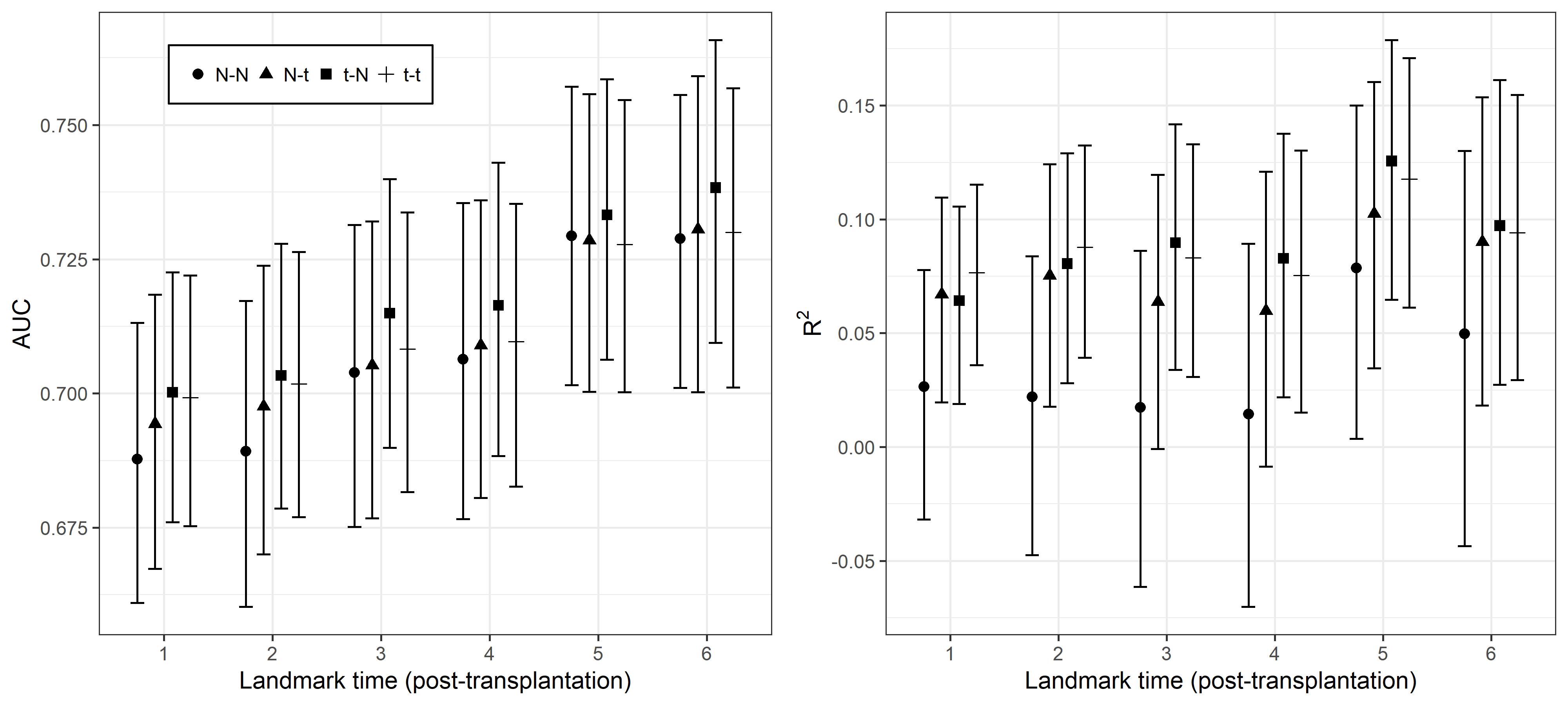 Figure 1
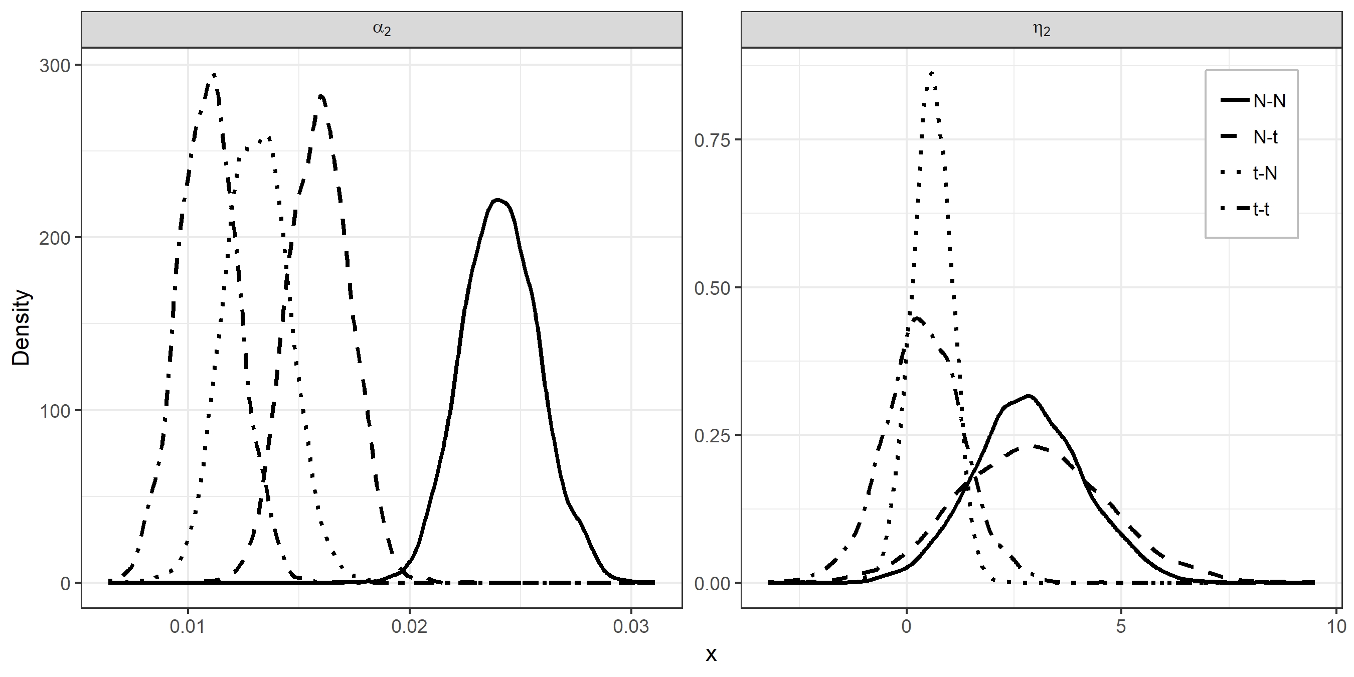 Figure 2
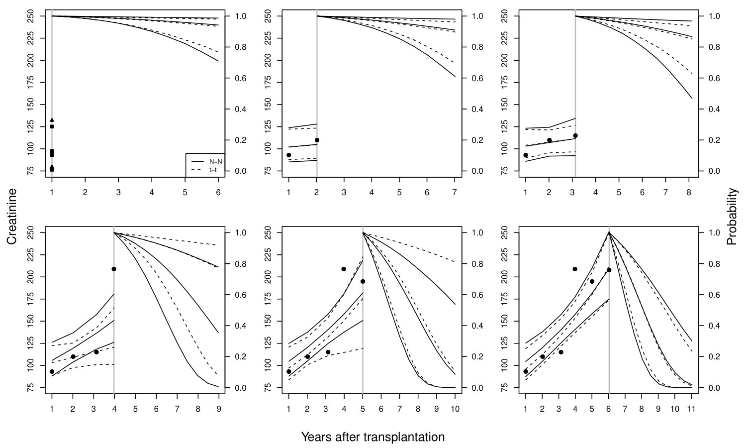 Figure 3
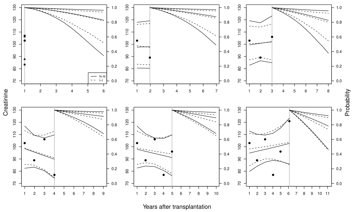 Figure 4
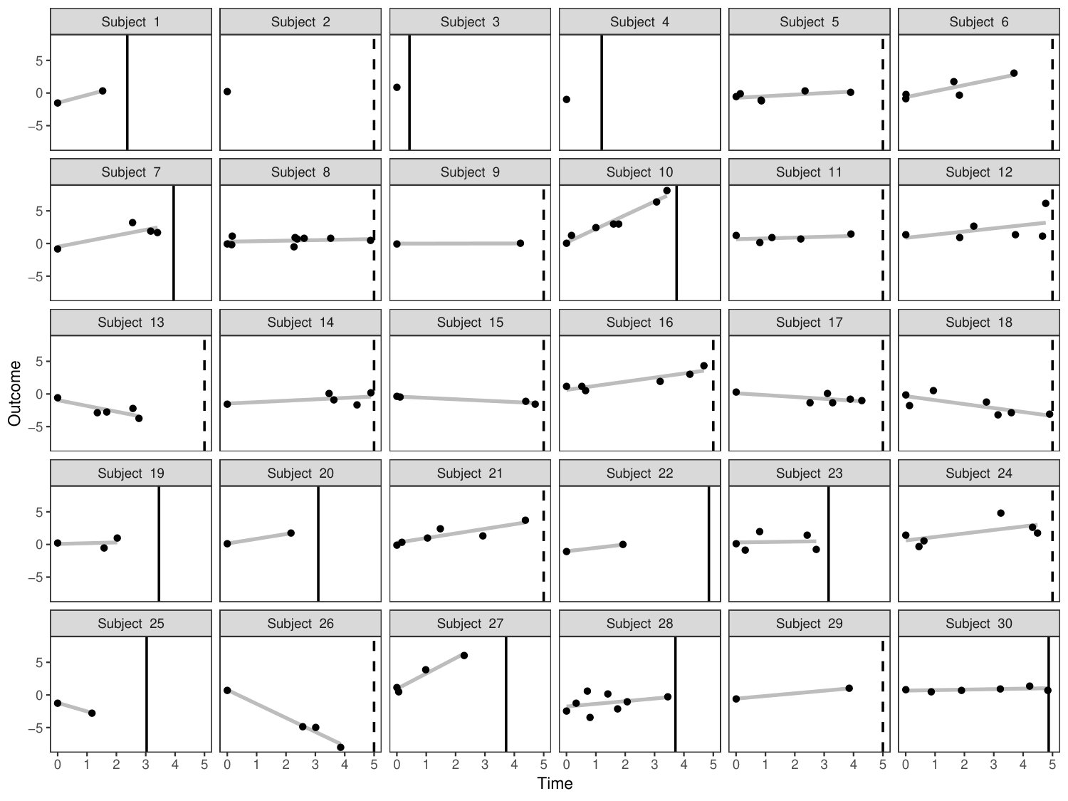 Figure 5
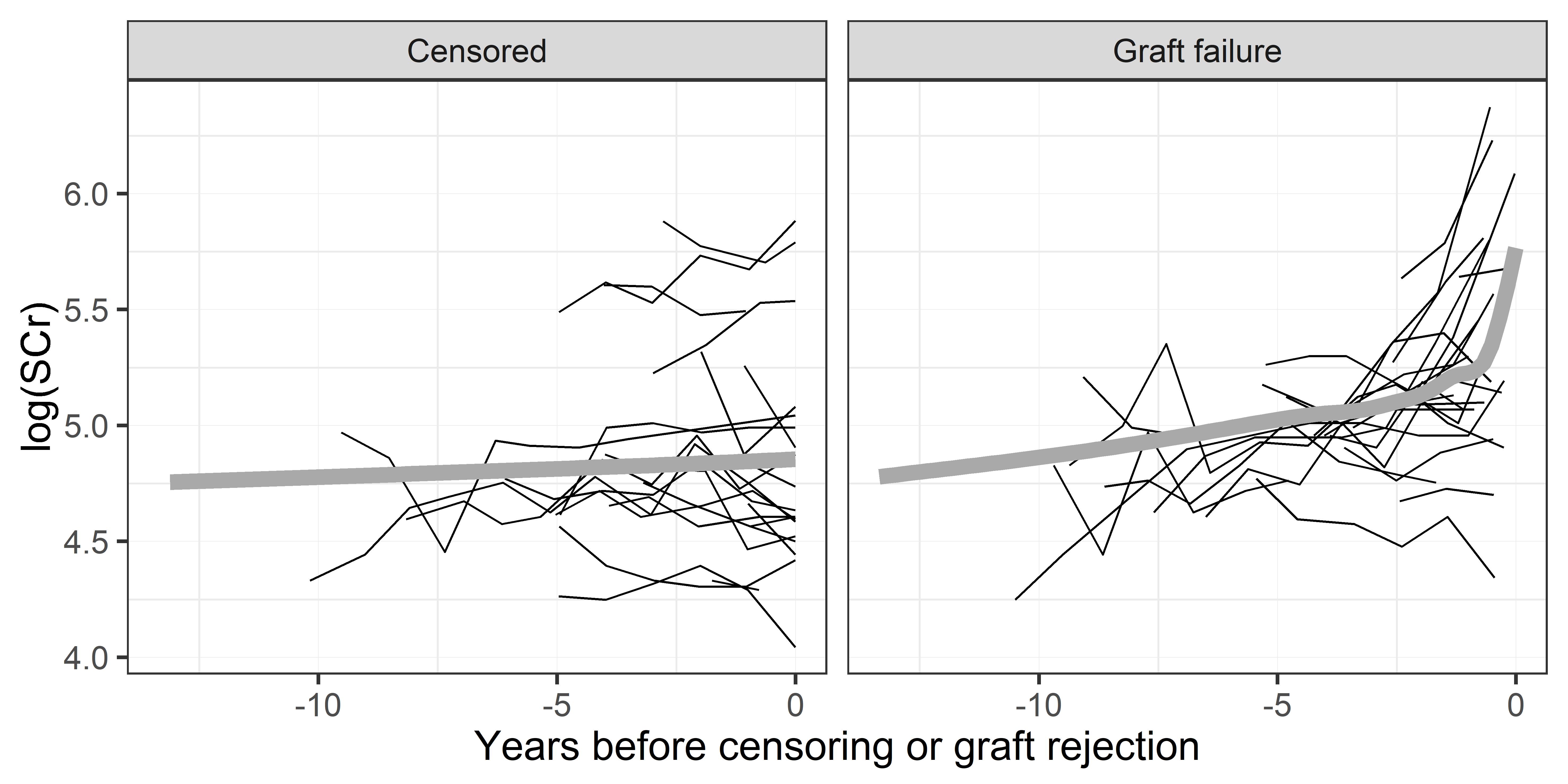 Figure 6
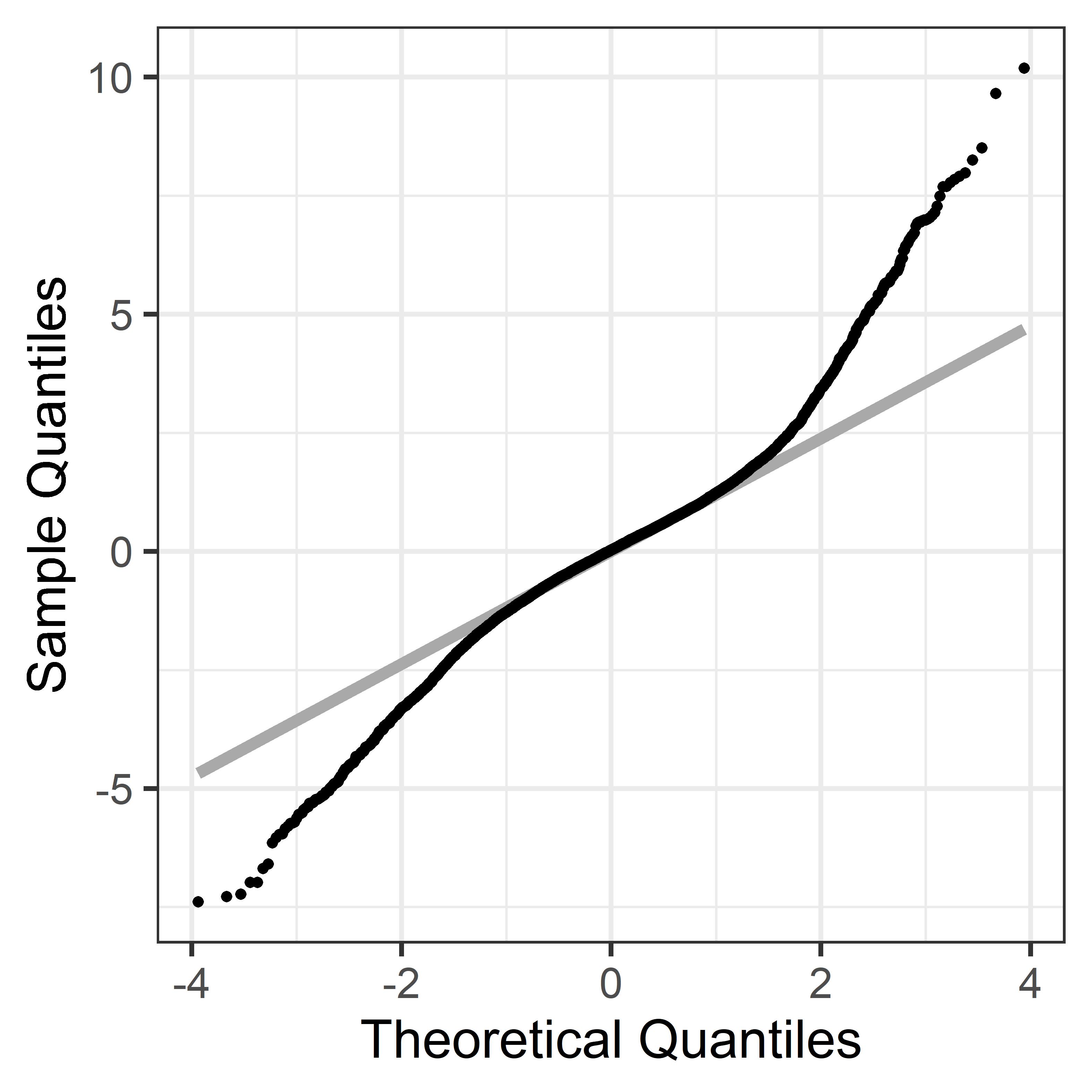 Figure 7
Peer Reviews
No public reviews on file for this paper yet. If you reviewed it on a platform where reviews are public (OpenReview, ICLR, NeurIPS, ICML), you can paste yours below so the community can read it here.
Videos
No videos yet. Explain this paper in a talk, walkthrough, or lecture? Add one.
Dynamic predictions of kidney graft survival
in the presence of longitudinal outliers
Özgür Asar
Marie-Cécile Fournier
INSERM UMR 1246 - SPHERE, Nantes University, Tours University, Nantes, France.
Etienne Dantan
INSERM UMR 1246 - SPHERE, Nantes University, Tours University, Nantes, France.
(* [email protected] [email protected])
Abstract
In kidney transplantation, dynamic predictions of graft survival may be obtained from joint modelling of longitudinal and survival data for which a common assumption is that random-effects and error terms in the longitudinal sub-model are Gaussian. However, this assumption may be too restrictive, e.g. in the presence of outliers, and more flexible distributions would be required. In this study, we relax the Gaussian assumption by defining a robust joint model with -distributed random-effects and error terms to get dynamic predictions of graft survival for the kidney transplant patients from the French DIVAT cohort. We take a Bayesian paradigm for inference and dynamic predictions and sample from the posterior densities. While previous research reported improved performances of robust joint models compared to the Gaussian version in terms of parameter estimation, dynamic prediction accuracy obtained from such approach has not been yet evaluated. Our results illustrate that estimates for the slope parameters in the longitudinal and survival sub-models are sensitive to the distributional assumptions. From a validation sample, calibration and discrimination performances appeared better under the robust joint models compared to the Gaussian version, illustrating the need to accommodate outliers in the dynamic prediction context.
Keywords: Dynamic prediction; kidney transplantation; longitudinal outliers; predictive accuracy; repeated measures; time-to-event
1 Introduction
In the context of chronic diseases, prediction scores of clinical events have become increasingly popular. These scores may help patients and physicians in a shared decision-making and facilitate the implementation of the P4-medicine (predictive, personalized, preventive and participative) (Flores et al., 2013) in clinical practice. Often measured to assess patients’ health evolution during the follow-up, longitudinal markers can be used to improve time-fixed (static) predictions obtained using only baseline information. Dynamic predictions are therefore defined as updated predictions, whenever any new data become available along the follow-up (Rizopoulos, 2012; Proust-Lima and Blanche, 2014).
In the statistical literature, there is a growing interest in methods to compute dynamic predictions. Among them, joint modelling of longitudinal and survival data is one of the most popular (Proust-Lima and Taylor, 2009; Rizopoulos, 2011; Taylor et al., 2013; Asar et al., 2015). Classically, survival outcomes are modelled using a Cox model with a time-varying frailty term, whereas the repeated measures are modelled using a mixed-effect model with Normally distributed random-effects and error terms. In longitudinal clinical studies, some observations may be highly apart from the others, and two types of outliers may be defined: i) at population level, outlying subjects who do not follow the typical population trend, ii) at individual level, outlying observations that do not follow the typical trajectory of an individual (Pinheiro et al., 2001; Wu, 2009). Gaussian assumption would not give appropriate weights to these individuals or observations, i.e. it would not be robust against outliers (Sutradhar and Ali, 1986; Lange et al., 1989).
In the context of kidney transplantation, a systematic review on predictive models emphasized the need for dynamic predictions (Kaboré et al., 2017). Since longitudinal measures of serum creatinine (SCr) have been demonstrated as associated with kidney graft failure (Fournier et al., 2016), we recently proposed to use them to obtain dynamic predictions of long-term kidney graft failure (Fournier et al., 2019). For the French kidney transplant cohort DIVAT (www.divat.fr), we obtained dynamic predictions of graft survival based on a joint model with Gaussian random-effects and error terms. Nevertheless, such dynamic predictions based on this joint model may be sub-optimal in presence of longitudinal outliers.
The objective of the current paper is to investigate possible impacts of longitudinal outliers on dynamic predictions of long-term kidney graft survival. We compare prognostic accuracies (discrimination and calibration) of the Gaussian and robust joint modelling approaches for the DIVAT patients. For the robust joint modelling, we relax the Gaussian assumption by postulating distributions for the random-effects and error terms. The robust model we consider is novel in the sense that it postulates independent distributions for the random-effects and error terms, and error terms are allowed to be independent within a subject. To the best of our knowledge, there is no work in the literature that considered such a joint model. For inference and dynamic predictions, we take a Bayesian paradigm and sample from the joint posterior densities. While several authors reported better performance of robust joint models compared to the Gaussian version in terms of parameter estimation, especially in terms of standard error estimation (Li et al., 2009; Huang et al., 2010; Sungduk and Albert, 2016; Baghfalaki et al., 2013, 2014), the advantages of robust joint modelling regarding individual dynamic predictions are yet to be explored.
The rest of the paper is organised as follows. In Section 2, we give details of the DIVAT data that motivates this work. Sections 3 introduces the general modelling framework, distributional assumptions and inferential procedures. Section 4 describes dynamic predictions for newcomer subjects and accuracy measures to evaluate prognostic capabilities of the models. In Section 5, we present a concrete application to the DIVAT data-set. Section 6 closes the paper.
2 DIVAT data
Data were extracted from the multicentric French kidney transplant cohort DIVAT (French Research Ministry: RC12_0452, last agreement No 13 334, No CNIL for the cohort: 891735). The inclusion criteria are: adult recipients who received a first or second renal graft from a living or heart-beating deceased donor, alive with a functioning graft at 1 year post-transplantation, and maintained under Tacrolimus and Mycofenolate. The aim is to predict graft failure risk in the chronic phase of transplantation. Therefore, time origin is selected as 1 year after transplantation. Graft failure is defined as the occurrence of any of the following events: return to dialysis, pre-emptive re-transplantation, or death with a functioning graft. Serum creatinine (SCr, measured in mol/L) is the longitudinal biomarker, with high values indicating worse kidney health. Following Fournier et al. (2019), the following set baseline covariates are considered: recipient age (Age: in years), history of cardiovascular disease (CV: yes/no), 3-month SCr (SCr3), occurrence of an acute rejection episode in the first year post-transplantation (AR: yes/no), pre-transplantation anti-class I immunisation (ACI: yes/no) and graft rank (GR: second/first). Follow-up time is the time-varying covariate.
The learning and validation samples are constructed based on two data extracts. While the first extract covers the period of 1 January 2000 – 31 August 2013, the second covers 1 September 2013 – 31 October 2016. Randomly chosen two-third of the first extract constitutes the learning sample (2,584 patients), whereas remaining portion of the first extract plus the whole data from the second extract constitute the validation sample (1,577+946 = 2,523 patients). Number of repeated measures ranged between 1 and 14 (with median of 4) for the learning sample. Spagetti-plots SCr (in log-scale) for a random sample of 60 patients from the learning sample are shown in Figure 1. For more details of the data, reader is referred to Fournier et al. (2019). The quantile-quantile plot displayed in Figure 2 indicates that there are considerable departures from the Gaussian assumption for the DIVAT data-set.
3 Joint modelling of longitudinal and survival outcomes
From Figure 2, we are not able to discern the source of heavy-tailedness, i.e. whether it is due to outlying individuals or outlying observations or both. Therefore, in what follows we consider a general modelling framework which postulates that both types of outliers may be present. Based on the posterior summaries for the degrees-of-freedom parameters for random-effects and error terms, we can then drop the heavy-tailedness assumption for the term for which Normality is indicated.
3.1 Notations and framework
To make inference, we assume to observe a sample of independent and identically distributed subjects with the data of . Here, is the set of longitudinal marker with the set of corresponding timings, ; the baseline explanatory variables; and the time elapsed between the origin and occurrence of the survival event. is typically right-censored, i.e. , where being the true survival time and the censoring time for subject . Therefore, an event indicator, , where denotes the indicator function, completes the survival information.
In this study, we consider the so-called shared-parameter version of the joint model Wulfson and Tsiatis (1997), based on two linked sub-models. The modelling framework can be defined as follows:
[TABLE]
Equation (1) corresponds to a linear mixed-effects model that defines the longitudinal process. The observed longitudinal measure, , is assumed to be a noisy version of the underlying continuous-time signal, , at time , with being the noise, or as often called measurement error. is a design matrix that consists of elements from and , and another design matrix that is typically structured as a subset of . and are population-averaged parameters and subject-specific random-effects (latent variables), respectively.
Equation (2) corresponds to a Cox model with time-varying frailty for the time-to-event. is the instantaneous risk of experiencing the event at time , and the baseline hazard. can be left un-specified as in Cox (1972), or specified parametrically using hazard function of a life-time distribution, e.g. for Weibull , or using piecewise-constants or splines; for details see Rizopoulos (2012). is a design matrix that is composed of elements from , and are the associated parameters. is the term that links features of underlying signal up to and including time , , and hazard function at time through a known link function and parameters . There are a number of choices for . Widely used examples include, among others, the current value parametrization, , or current value and rate of change parametrization, ; for other parametrizations, see (Rizopoulos, 2012).
3.2 Distributional assumptions
Standard joint models assume that and are both zero-mean Gaussian, such that and . The terms are further assumed to have the following properties, and for . Gaussian assumption might be too restrictive for some real-life applications, because the data-sets typically consist of subjects that exhibit outlying behaviours.
Pinheiro et al. (2001) discuss two types of longitudinal outliers:
- outlying individuals, and 2) outlying observations within individuals. Examples of outlying individuals include subjects with very high/low health status at baseline, and/or with rapid progression. In other words, outlying individuals correspond to outliers in . Examples of outlying observations might be a few observations that are quite different than the rest of the observations for a given individual. In other words, outlying observations correspond to outliers in . Figure 3 displays simulated realisations from a robust joint model. As expected, most of the subjects are homogeneous, while a few subjects seem to have extreme trajectory or extreme observations. For instance, subjects 10, 26 and 27 seem to have relatively higher slopes compared to the rest. Fourth observation for subject 24 seems to deviate more around the individual line compared to the other observations for the same subject. Similar features can also be seen for the DIVAT data-set: Figure 1 illustrates subjects with high level of SCr at baseline, with rapid progression, and with a few observations that seem different from the rest of the observations for the same subjects.
To accommodate the aforementioned outliers, the Gaussian assumption for and can be relaxed using distribution that would give lower weights to outliers. distribution can be specified using the variance mixtures as and , where and are inverse-Gamma random variables, such that and , with the following properties, , for , , and . With these specifications, one would obtain and , with the following properties, and , for . Note that the conditionals on the mixing variates are still Normal such that and . and are the so-called degree-of-freedom parameters, and it is well known that if such a parameter converges to infinity, distribution converges to the Gaussian.
To the best of our knowledge, there is no work in the literature that considered robust joint modelling with the above properties. Taylor et al. (2013), Li et al. (2009) and Huang et al. (2010) considered robust joint modelling with Normally distributed and -distributed with fixed degree-of-freedom parameters. Sungduk and Albert (2016) considered Normally distributed , and generalised -distributed . Baghfalaki et al. (2013, 2014) considered our model with . Note that under their specification, the property, for , does not hold, as is shared across ’s. Among these works, only Taylor et al. (2013) considered dynamic predictions, whereas the rest focused on parameter estimation.
3.3 Bayesian inference
In this section, we present inference for the joint model with -distributed and terms. Inference for the model with at least one of these terms being Gaussian, or being -distributed based on , are just special cases.
Let with ; ; ; with and as before; with and as before; with as before; ; with ; the parameters of ; with as before. The joint posterior density of the parameters and latent variables can be written as
[TABLE]
with being a general notation for probability density function. The first distribution on the right-hand side of (3.3), , is based on the longitudinal sub-model (1), and is constructed based on univariate Normal distributions such that
[TABLE]
The second term is based on the survival sub-model (2), and constructed by
[TABLE]
where being the survival function, defined as . As mentioned in Section 3.2, is constructed based on , and and are based on inverse-Gamma distributions, and , respectively. corresponds to the joint prior distribution of the parameters. We assume independent priors for the parameters such that
[TABLE]
are given zero-mean Cauchy prior with scale parameter of 5, , whereas is given . is decomposed as , where is diagonal matrix of scale parameters that are specific to , and is in the form of a correlation matrix. Elements of are given half-Cauchy priors with scale of 5, , whereas elements of are given LKJ prior with the parameter of 2, . and are given uniform priors, between 2 and 100. is given . Log-transformed elements of and elements of and are given .
Samples from the joint posterior (3.3) are drawn using HMC (Neal, 2011), specifically using the NUTS algorithm (Hoffman and Gelman, 2014), that is an adaptive version of HMC. Methods are implemented in the R package robjm (github.com/ozgurasarstat/robjm) (R Core Team, 2018), that internally uses the so-called HMC engine Stan (Carpenter et al., 2017) through the RStan package (Stan Development Team, 2018).
4 Dynamic predictions
4.1 Definition
Our target of inference for a newcomer subject is the prediction of subject-specific conditional failure probability between time points and given that the patient did not experience the event until time point , i.e. , and subject-specific data recorded up to and including time :
[TABLE]
where is called the lead-time or forecast horizon. The conditional survival probability in (4.1) could be obtained as
[TABLE]
where consists of all the parameters. For the a new subject, we would not have samples from , that are readily obtained during the inference step. We can draw the latent variables, , from
[TABLE]
using the MC samples of the parameters obtained from ; see (3.3). One would obtain dynamic predictions by updating to , if subject is still at risk at time (such that ) by incorporating any new data recorded for her/him in the time interval .
4.2 Accuracy measures for dynamic predictions
A prediction score, whether dynamic or not, requires good properties of discrimination and calibration in order for having a practical use in personalized medicine (Steyerberg et al., 2010). Methods to assess these properties have already been extensively published (Graf et al., 1999; Gerds and Schumacher, 2006; Heagerty et al., 2000) and have recently been extended to dynamic predictions (Schoop et al., 2008; Blanche et al., 2015; Fournier et al., 2018).
A widely used discrimination measure is the Area Under the Receiver Operating Characteristics Curve (AUC) that aims to assess how the predictions distinguish between a patient who has the event from another patient who does not. In a dynamic prediction context, AUC is calculated for each landmark time-point , with a forecast horizon of , such that
[TABLE]
where and are indices for two randomly selected subjects. We use the estimator of Blanche et al. (2015) for taking into account right-censoring. Higher AUC values indicate better discrimination.
Brier score is one of the widely used measure to globally assess the prognostic performances. A disadvantage of the Brier score is that it depends on the marginal failure probabilities that could potentially take different values at different landmark times, and thus can be misleading in the dynamic prediction context. Fournier et al. (2018) proposed an -type criterion that builds on the Brier score by adjusting it with the marginal failure probability such that
[TABLE]
where is the Brier score and the Brier score for the reference model that does not use any subject-specific information. Higher indicates better performance.
As shown in Fournier et al. (2018), both Brier score and the -type criterion measure calibration and discrimination simultaneously. We therefore also use calibration plots to solely check the calibration properties of the predictions. The calibration is described as comparing predicted values within subgroups, e.g. defined from deciles of predictions for the DIVAT application, to observed event survival that is computed using the Kaplan-Meier method. From a Bayesian perspective, we have calculated deciles for each of element of the MC samples of dynamic predictions.
5 Application to the kidney transplantation data
5.1 Joint modelling for the learning sample
Following Fournier et al. (2019), the following joint model is fitted to the learning data:
[TABLE]
where , and stands for transplantation period: before 31 December 2007 versus after January 2008. No baseline covariates were included in (8) since SCr evolution is on the causal pathway between baseline factors and graft failure risk as discussed in Fournier et al. (2019). Besides, it was confirmed in the web supplementary material of Fournier et al. (2019) that inclusion of baseline covariates in the longitudinal sub-model did not improve predictive performances. Note that the current value and rate of change parametrization is suggested by Figure 1: increase in the mean SCr level is higher for the graft failure group compared to the censored group, and for the former group there is an acceleration in the SCr increase towards the event.
In the following, we will distinguish between four joint models for the DIVAT data-set based on the following distributional assumptions: Normally distributed and Normally distributed ( model), -distributed and -distributed (), Normally distributed and -distributed (), -distributed and Normally distributed (). Our general strategy would be to fit the model when there is evidence against Normal, and check the posterior summaries of the degrees-of-freedom parameters. As mentioned before, this approach is due to the fact that we do not know the source of heavy-tailedness in the standardised marginal residuals (see Figure 2). If results for any of the degrees-of-freedom parameters indicates that Normal assumption is reasonable, we then switch to or model. As will be discussed in the next paragraph, for the DIVAT application, model does not indicate Normality to either of the or terms. Therefore, we include the and models for the sake of seeing the likely effects of wrongly assuming any of or as Normal. For each of the models, 4 chains with lengths of 2,000 were started from random initials. For each chain, first halves were considered as warm-up that results MC samples of 4,000 for each model. Convergence of the chains were checked using trace-plots, density plots for the chains, and R-hat statistic of Brooks and Gelman (1997).
Table 1 presents posterior summaries for each of the 4 joint models, specifically the 2.5%th, 50%th and 97.5%th percentiles, of the MC samples. Results for and under the model imply that both and reflect heavier tails than the Gaussian. When we let both and being Normally distributed (i.e. the model), the population-averaged slope, , is largely over-estimated, compared to the model. When we only let the error terms being -distributed (i.e. the model), this over-estimation gets milder. The results of under the model are the most similar to those of the model. These can be explained as the following: profiles for subjects who had extreme progression (high slopes) are better captured by the -distributed terms. However, when the error term is assumed to be Normal ( model), all the outlying behaviours are forced to be in , hence we obtained somewhat over-estimated . Additionally, is largely over-estimated by the models with Normally distributed regardless of being Normal or . This can also be explained by better capturing subject-specific slopes that in turn would results better predictions for . Smoothed posterior densities for and are presented in Figure 4. Scatter-plots of the posterior quantiles of and to compare the models are presented in Figures of the supplementary material. Note that the differences between the models are more apparent for .
5.2 Dynamic predictions for the validation sample
5.2.1 Accuracy measures
Dynamic predictions are calculated at six post-transplantation landmark times: . A clinically meaningful forecast window of 5 years is considered, i.e. . Table 2 is the frequency table regarding subjects who were at risk at the landmark times, subjects who had the event, and who were censored within the forecast horizons, and subjects who survived beyond the forecast horizons.
Posterior summaries of the AUC and R2 are displayed in Figure 5. Calibration plots are dislayed in Figures of the supplementary material, whereas the estimated slopes fit to predicted risk versus observed risk are reported in Table 3. Note that as mentioned in Fournier et al. (2018), can take negative values. Globally, discrimination is good for all the models, AUC’s increase with landmark times, and calibration performances appear reasonable. More interestingly, comparing the models, we observe the best results under the model in terms of AUC and . It is followed by the model and the model. The has the worst performance. In terms of calibration, again the and models appeared the best two. Whereas in landmark times , model had higher slope estimates compared to the model, for the later times the estimates are almost the same.
We also calculated 2.5th, 50th and 97.5th percentiles of the dynamic predictions for each individual for each landmark times. Scatter-plots of these statistics are displayed in Figures of the supplementary material. It can be seen, e.g. based on the medians, that there are some subjects for whom the models quite disagree, e.g. see the dots that are above the lines. One can deduce that there are some subjects (e.g. outlying subjects) whose dynamic predictions benefit from the robust joint model with distributions, especially -distributed terms.
5.2.2 Results for two patients
We present 5-year dynamic predictions for two patients from the validation sample. They are the same subjects presented in Fournier et al. (2019). The first patient (Figure 6) was a female, aged 51 years, transplanted in 2005 for the first time, without history of a cardiovascular disease, immunized against HLA class I, with a SCr measurement at 3 months post-transplantation of 88 mol/L, and without acute rejection episode in the first year post-transplantation. The recipient was returned to dialysis at 9.34 years after transplantation. The second patient (Figure 7) was a female, aged 60 years at transplantation, transplanted in 2007 for the second time, without history of a cardiovascular disease, immunized against HLA class I, and a SCr measurement at 3 months post-transplantation of 100 mol/L, and at least one acute rejection episode in the first year after transplantation. The recipient was still alive with a functioning graft at 10.14 years post-transplantation. Figures 6 & 7 only present the results under the and models, whereas results under all the four models are presented in Figures 17 & 18 of the supplementary material. For these patients, dynamic predictions obtained under the models generally agree. There is a notable difference for the first patient in the fourth landmark time-point; see mid-right panel of Figure 6. The difference is due to the fourth SCr measurement that is a typical example of outlying observations: the fourth was 209, whereas the first three were 93, 110, and 115. and assumptions overreact and produce considerably lower survival probabilities compared to the and . Median (2.5% and 97.5% percentiles of the MC samples) of the survival probabilities for 8.97 years after transplantation, i.e. , were 0.35 (0.01, 0.78), 0.35 (0.00002, 0.82), 0.74 (0.27, 0.92), 0.77 (0.08, 0.92) under , , and models, respectively. Note that the patient had graft failure at year 9.3, i.e. . The fifth measurement for the same subject is 195 that is closer in magnitude to the fourth measurement compared to the first three. , and models correctly react to the fifth measurement and update the predictions accordingly. However, it model seems to produce somewhat higher median probabilities compared to these three models.
6 Discussion
In this work, we considered dynamic predictions of kidney graft survival using joint modelling of longitudinal and survival outcomes. We mainly focused on how the distributional assumptions would impact the predictions: widely used Normal distribution was compared against . The proposed joint model with distributional assumptions is novel, as no work in the literature considered such a general model. Bayesian methods were considered for estimation and dynamic predictions. The proposed methods are implemented in the R package robjm. Methods are applied to data for kidney transplant patients from the French cohort DIVAT. Impacts of distributional assumptions on dynamic prediction performances were inspected through accuracy measures and predictions on two individuals are illustrated.
Regarding the DIVAT data-set, degree-of-freedom results indicated that there are both outlying individuals and outlying observations. We observed important differences between the standard and the robust joint models. The population averaged slope in the mixed-effects sub-model and the association parameter for the individual rate of change in the survival sub-model were largely over-estimated by the Gaussian joint model. In terms of dynamic predictions, we observed better calibration and discrimination for the robust joint models. Intermediate joint models, i.e. the and assumptions, suggest that outlying subjects have greater impact on dynamic predictions if they are not considered compared to outlying observations. Regarding individual dynamic predictions, robust models produced better results for the patient with outlying observation, whereas the two models produced similar results for the subject with no outlying observation.
Our current work voluntarily does not include a simulation study. Indeed, the objective is to present a case-study on predicting kidney graft failure risk, specifically for the patients in the DIVAT cohort. We clearly illustrated that considering longitudinal outliers have an impact on prognostic accuracy in the kidney transplantation context. Our modelling strategies may be applicable to others clinical contexts. When comparing the four joint models, we also voluntarily do not consider metrics for model selection. Indeed, since we are mainly interested in dynamic predictions, we compare the models using predictive accuracy measures obtained from a validation data-set.
In our robust joint model proposal, we considered symmetric distribution as an alternative to the Gaussian. Given that distributional assumptions might have considerable impacts on dynamic predictions, it would be worth to study other distributions than symmetric , e.g. skew-. We considered joint modelling framework with the shared-parameter formulation to link the longitudinal and survival sub-models. Performances of other methods, e.g. latent class joint modelling (Proust-Lima et al., 2014), Cox model with time-varying covariates, or landmarking methods (van Houwelingen, 2007), in the presence of longitudinal outliers would also be interesting to investigate. Diagnostics tools for checking the appropriateness of distributional assumptions for non-Gaussian joint models would be interesting. In this study, this was secondary to us, since our aim was to inspect if we can improve the dynamic predictions obtained from the widely used Normal assumption, and checked this using accuracy measures for the validation sample.
Fournier et al. (2019) previously presented dynamic predictions for the DIVAT patients using the joint model with a frequentist point of view. We are able to re-produce their results using our model. The AUC and values presented in (Fournier et al., 2019) are higher than those presented in the current paper. The reason for this is that they used median of the MC samples to obtain the point estimates and frequentist methods to obtain the associated intervals rather than obtaining MC samples of the accuracy measures. Yet, following their approach, we are able to obtain the values they presented.
In conclusion, this study presents improved dynamic predictions of kidney graft failure based on robust joint modelling framework. The most important component to obtain improved predictions seems the random-effects terms. Nonetheless, even letting only the error term being -distributed improves predictions compared to the Gaussian model. We prefer working with the model, since i) it consists of the and models as special cases, ii) it is one of the best in terms of accuracy measures, iii) it provides a good compromise between the two special cases as presented for the first patient. The predictions based on the model will be deployed into the DynPG Shiny application of Fournier et al. (2019) (available at https://shiny.idbc.fr/DynPG) that is currently based on Gaussian joint modelling. This would allow physicians and patients get benefit from our methods.
Acknowledgements
Dr. Özgür Asar was funded by the French Embassy to Turkey for a visit to The University of Nantes, which enabled great progress for the current work. Helpful discussions with Dr. Jonas Wallin (Lund University), Prof. Peter Diggle (Lancaster University) and Dr. Yohann Foucher (Nantes University) are greatfully acknowledged. The analysis and interpretation of data collected from the French DIVAT (Données Informatisées et VAlidées en Transplantation) cohort* (www.divat.fr, No. CNIL 914184) are the responsibility of the authors. We wish to thank members of the data manager of the DIVAT cohort (Clarisse Kerleau) and clinical research assistant team (S. Le Floch, A. Petit, J. Posson, C. Scellier, V. Eschbach, K. Zurbonsen, C. Dagot, F. M’Raiagh, V. Godel, X. Longy, P. Przednowed). We are also grateful to Roche Pharma, Novartis and Sanofi laboratories for supporting the DIVAT cohort as the CENTAURE foundation (www.fondation-centaure.org).
- DIVAT cohort collaborators (Medical Doctors, Surgeons, HLA Biologists): Nantes: G. Blancho, J. Branchereau, D. Cantarovich, A. Chapelet, J. Dantal, C. Deltombe, L. Figueres, C. Garandeau, M. Giral, C. Gourraud-Vercel, M. Hourmant, G. Karam, C. Kerleau, A. Meurette, S. Ville, C. Kandell, A. Moreau, K. Renaudin, A. Cesbron, F. Delbos, A. Walencik, A. Devis; Paris-Necker: L. Amrouche, D. Anglicheau, O. Aubert, L. Bererhi, C. Legendre, A. Loupy, F. Martinez, R. Sberro-Soussan, A. Scemla, C. Tinel, J. Zuber; Nancy: P. Eschwege, L. Frimat, S. Girerd, J. Hubert, M. Ladriere, E. Laurain, L. Leblanc, P. Lecoanet, J-L. Lemelle; Lyon E. Hériot: L. Badet, M. Brunet, F. Buron, R. Cahen, S. Daoud, C. Fournie, A. Grégoire, A. Koenig, C. Lévi, E. Morelon, C. Pouteil-Noble, T. Rimmelé, O. Thaunat; Montpellier: S. Delmas, V. Garrigue, M. Le Quintrec, V. Pernin, J-E. Serre.
The reference list from the paper itself. Each links out to its DOI / PubMed record.
- 1Asar et al. (2015) Ö. Asar, J. Ritchie, P. A. Kalra, and P. J. Diggle. Joint modelling of repeated measurement and time-to-event data: an introductory tutorial. International Journal of Epidemology , 44(1):334–344, 2015.
- 2Baghfalaki et al. (2013) T. Baghfalaki, M. Ganjali, and D. Berridge. Robust joint modeling of longitudinal measurements and time to event data using normal/independent distributions: A bayesian approach. Biometrical Journal , 55(6):844–865, 2013.
- 3Baghfalaki et al. (2014) T. Baghfalaki, M. Ganjali, and R. Hashemi. Bayesian joint modeling of longitudinal measurements and time-to-event data using robust distributions. Journal of Biopharmaceutical Statistics , 24(4):834–185, 2014.
- 4Blanche et al. (2015) P. Blanche, C. Proust-Lima, L. Loubère, C. Berr, J-F. Dartigues, and H. Jacqmin-Gadda. Quantifying and comparing dynamic predictive accuracy of joint models for longitudinal marker and time-to-event in presence of censoring and competing risks. Biometrics , 71(1):102–113, 2015.
- 5Brooks and Gelman (1997) S. P. Brooks and A. Gelman. General methods for monitoring convergence of iterative simulations. Journal of Computational and Graphical Statistics , 7:434–455, 1997.
- 6Carpenter et al. (2017) B. Carpenter, A. Gelman, M. D. Hoffman, D. Lee, B. Goodrich, M. Betancourt, M. Brubaker, J. Guo, P. Li, and A. Riddell. Stan: A probabilistic programming language. Journal of Statistical Software , 76(1):1–32, 2017.
- 7Cox (1972) D. R. Cox. Regression models and life-tables. Journal of the Royal Statistical Society. Series B (Methodological) , 34(2):187–220, 1972.
- 8Flores et al. (2013) M. Flores, G. Glusman, K. Brogaard, N. D. Price, and L. Hood. P 4 medicine: How systems medicine will transform the healthcare sector and society. Personalized Medicine , 10(6):565–576, 2013.