Total positivity in exponential families with application to binary variables
Steffen Lauritzen, Caroline Uhler, Piotr Zwiernik

TL;DR
This paper explores multivariate totally positive exponential families, highlighting their properties, conditions for maximum likelihood estimation, and applications to graphical models and binary data analysis.
Contribution
It characterizes MTP2 exponential families, establishes conditions for MLE existence, and introduces a new algorithm for MTP2 Ising models.
Findings
MLE exists with as few as d observations in binary MTP2 models
MTP2 serves as an implicit regularizer leading to sparsity in graphical models
Proposed a globally convergent algorithm for MTP2 Ising models
Abstract
We study exponential families of distributions that are multivariate totally positive of order 2 (MTP2), show that these are convex exponential families, and derive conditions for existence of the MLE. Quadratic exponential familes of MTP2 distributions contain attractive Gaussian graphical models and ferromagnetic Ising models as special examples. We show that these are defined by intersecting the space of canonical parameters with a polyhedral cone whose faces correspond to conditional independence relations. Hence MTP2 serves as an implicit regularizer for quadratic exponential families and leads to sparsity in the estimated graphical model. We prove that the maximum likelihood estimator (MLE) in an MTP2 binary exponential family exists if and only if both of the sign patterns and are represented in the sample for every pair of variables; in particular, this implies…
Click any figure to enlarge with its caption.
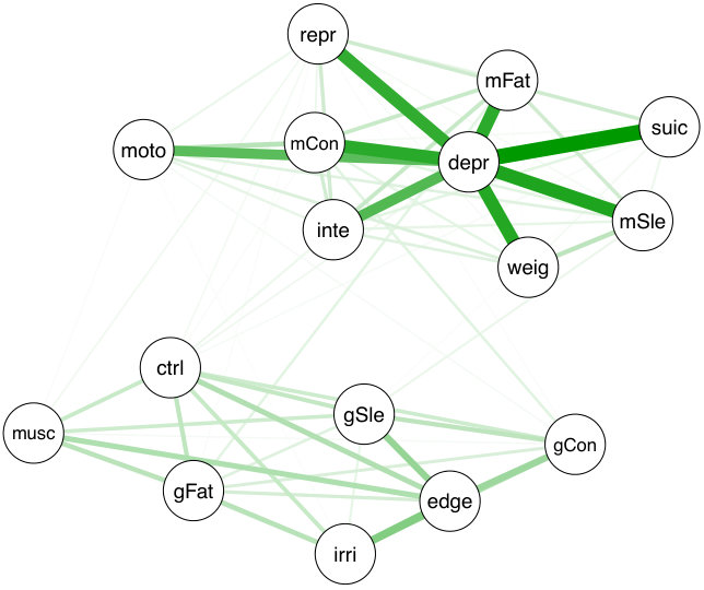 Figure 1
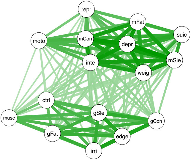 Figure 2
Peer Reviews
No public reviews on file for this paper yet. If you reviewed it on a platform where reviews are public (OpenReview, ICLR, NeurIPS, ICML), you can paste yours below so the community can read it here.
Videos
No videos yet. Explain this paper in a talk, walkthrough, or lecture? Add one.
Total positivity in exponential families with application to binary variables
Steffen Lauritzenlabel=e1][email protected] [
Caroline Uhlerlabel=e2][email protected] [
Piotr Zwiernik label=e3][email protected] [ University of Copenhagen\thanksmarkm1, Massachusetts Institute of Technology\thanksmarkm2,
ETH Zurich\thanksmarkm2 and Universitat Pompeu Fabra\thanksmarkm3
Department of Mathematical Sciences
University of Copenhagen
Copenhagen, Denmark
Laboratory for Information and Decision Systems,
and Institute for Data, Systems, and Society
Massachusetts Institute of Technology
Cambridge, MA, USA
Department of Economics and Business
Universitat Pompeu Fabra
Barcelona, Spain
Abstract
We study exponential families of distributions that are multivariate totally positive of order (), show that these are convex exponential families, and derive conditions for existence of the MLE. Quadratic exponential familes of distributions contain attractive Gaussian graphical models and ferromagnetic Ising models as special examples. We show that these are defined by intersecting the space of canonical parameters with a polyhedral cone whose faces correspond to conditional independence relations. Hence serves as an implicit regularizer for quadratic exponential families and leads to sparsity in the estimated graphical model. We prove that the maximum likelihood estimator (MLE) in an binary exponential family exists if and only if both of the sign patterns and are represented in the sample for every pair of variables; in particular, this implies that the MLE may exist with observations, in stark contrast to unrestricted binary exponential families where observations are required. Finally, we provide a novel and globally convergent algorithm for computing the MLE for Ising models similar to iterative proportional scaling and apply it to the analysis of data from two psychological disorders.
60E15, 62H99,
15B48,
graphical models,
Ising model,
log-supermodular distributions,
positive dependence,
exponential families,
keywords:
[class=MSC]
keywords:
\setattribute
journalname
\startlocaldefs
\endlocaldefs
,
and
1 Introduction and motivation
This paper discusses exponential families and, in particular, binary graphical models with a special form of positive dependence. Total positivity is a strong form of positive dependence that has become an important concept in modern statistics; see, e.g., [14, 22]. This property (also called the property) appeared in the study of stochastic orderings, asymptotic statistics, and in statistical physics [19, 30]. Families of distributions with this property lead to many computational advantages [8, 16, 31] and they are a convenient shape constraint in nonparametric statistics [32]. They also became a useful tool in modelling with latent variables; see [9] for an overview. In particular, in [4] the property explicitly appeared in the description of the binary latent class model.
In the Gaussian setting, the property was shown to simplify inference [5, 27]. In this case the property is equivalent to the covariance matrix being an inverse M-matrix, which is a linear constraint on the concentration matrix. This led Slawski and Hein [33] to propose efficient learning procedures based on convex optimization; see also [11, 17, 25]. The present paper develops similar results for exponential families with special emphasis on models for binary variables, including ferromagnetic Ising models. Our main results are the following:
- •
We show in Section 3 that the property is given by a convex constraint in an exponential family and use convex optimization theory to derive necessary and sufficient conditions ensuring than an estimate maximizes the likelihood. For a quadratic exponential family, including the Ising model for binary variables, the KKT conditions yield sparsity in the associated matrix for interaction potentials.
- •
We show in Section 4 that the KKT conditions ensure context-dependent conditional independence restrictions and that for binary variables the MLE exists under if and only if both of the sign patterns and are represented in the sample for every pair of variables. This ensures the minimal sample size for the MLE to exist be of order rather than where is the number of variables considered.
- •
We show — also in Section 4 — that adding conditional independence assumptions by further assuming a graphical model, reduces this condition to hold for pairs of vertices that are neighbours in the graph, reducing the order of the minimal sample size to be the maximal clique size of the graph.
- •
We show — also in Section 4 — that for symmetric binary distributions, including ferromagnetic Ising models with no external field, presence of just one of the sign patterns and for every pair ensures existence of the MLE;
- •
We develop — in Section 5 — a novel IPS type algorithm for calculating the MLE in a ferromagnetic Ising model that is shown to be globally convergent.
The remainder of this paper is structured as follows: In Section 2 we formally introduce distributions and associated notation.
In Section 6 we apply our results to the analysis of two psychological disorders, showing that the resulting graphical model is highly interpretable and consistent with domain knowledge.
2 Preliminaries
Let be a finite set and let be random variables with labels in . We consider the product space , where is the state space of , inheriting the order from . In this paper, the state spaces are either discrete (finite sets) or open intervals on the real line.
Assumption 1**.**
All distributions are assumed to have densities with respect to the product measure , referred to as the base measure, where is the counting measure if is discrete, and is the Lebesgue measure giving length 1 to the unit interval if is an open interval.
We note that any other equivalent product measure can be used as base measure without affecting the property as defined below.
A function on is said to be multivariate totally positive of order () if
[TABLE]
where and denote the elementwise minimum and maximum, i.e.,
[TABLE]
These inequalities are non-trivial only if are not comparable, that is, neither nor . For , a function that is is simply called totally positive [22]. We say that or the distribution of is if its density function is .
For strictly positive distributions, can be verified by checking that (2.1) holds for that are not comparable and differ in exactly two coordinates; c.f. [22, Proposition 2.1]. We call such pairs elementary and denote the set of all elementary pairs by . For more details on distributions, see [22] and [18].
3 Totally positive exponential families
We first consider for exponential families and show that maximum likelihood estimation for exponential families under leads to a convex optimization problem. We then discuss conditions for the existence of the MLE and finally specialize these results to quadratic exponential families, which include as prominent examples the Gaussian distribution and the Ising model.
3.1 Convexity of totally positive exponential families
Consider an exponential family with density satisfying
[TABLE]
with sample space , sufficient statistics and base measure . Assume that the family is minimally represented, i.e. that almost surely implies , and that the family is regular so that the space of canonical parameters
[TABLE]
is an open convex set.
Assumption 2**.**
Throughout, we assume that there exists such that is a product distribution, or equivalently,
[TABLE]
Since every distribution in an exponential family can act as the base distribution, we can then pick as the base measure. It then holds that
[TABLE]
We say that such an exponential family has a product base.
All exponential families that contain a full independence distribution admit a product base. This includes all models discussed in this article and in particular Gaussian graphical models and log-linear models.
For an exponential family of the form (3.1) and any two we define
[TABLE]
The density is if and only if for all elementary pairs in . For exponential families with a product base it holds that
[TABLE]
which is an affine function in .
Definition 3.1**.**
The set of totally positive canonical parameters is the subset of canonical parameters for which the density is .
Since is given by the linear inequalities for all , we immediately get the following result.
Theorem 3.2**.**
The of totally positive canonical parameters is a convex set that is relatively closed in .
We note that this result holds also for exponential families without a product base. However, in that case the set of canonical parameters may be empty.
In [25] we considered the Gaussian setting and showed that is a convex cone. By essentially the same argument, this extends to discrete Gaussian distributions over , which were introduced in [1]. More generally, we obtain the following result.
Proposition 3.3**.**
The set is obtained by intersecting with a closed convex cone , whose dual cone is the closure of the cone generated by the set
[TABLE]
Proof.
The set of inequalities , one for each elementary pair , defines a convex cone in . We have for all if and only if for all in the cone generated by the set ; denote this cone by . This shows that and so . The latter is equal to the closure of by the standard theory of convex cones; see, for example, [13, Section 2.6.1]. ∎
Remark 3.4**.**
When is finite, i.e. for log-linear models, Proposition 3.3 implies that is polyhedral. Since is polyhedral also in the Gaussian setting, finiteness of is not a necessary condition. In fact, we will show in Proposition 3.6 that is polyhedral for any quadratic exponential family. When is polyhedral, then every face of intersected with corresponds to the distributions in an exponential subfamily.
3.2 The MLE and its existence
An important consequence of Theorem 3.2 is that any exponential family is a convex exponential family and thus the maximum likelihood estimator (MLE), if it exists, is uniquely defined; see [7, Section 9.4].
Let denote a sample of size and let be the average of the corresponding sufficient statistics. Let denote the interior of , the convex support of the sufficient statistics. Then by the general theory of exponential families [7], the MLE exists if and only if lies in , in which case it is uniquely defined by
[TABLE]
The following theorem extends this result to a characterization of existence of the MLE for the subfamily of distributions. By Proposition 3.3 there exists a closed convex cone such that the space of all canonical parameters is given by . We define
[TABLE]
as the Minkowski sum of with the dual of ; c.f. Proposition 3.3.
Theorem 3.5**.**
Let be a minimally represented regular exponential family. Then the MLE based on exists in the submodel if and only if , in which case is uniquely defined by
- (a)
primal feasibility: , 2. (b)
dual feasibility: with , 3. (c)
complementary slackness: .
Proof.
The maximum likelihood estimation problem can be formulated as the following optimization problem:
[TABLE]
This is a convex optimization problem, since is convex on . The Lagrangian is
[TABLE]
where . Let denote the conjugate dual of with domain . Then
[TABLE]
and hence the dual optimization problem is given by
[TABLE]
The MLE exists if and only if the primal and dual problems are feasible. The primal problem is feasible by the assumption . The dual problem is feasible if and only if . The characterization of the MLE then follows from the KKT conditions. ∎
As in the Gaussian case, complimentary slackness imposes sparsity in the MLE . This property makes exponential families potentially useful in high dimensional contexts. Before we discuss this in further detail, we shall consider the case of a quadratic exponential family, including the Gaussian case and Ising models.
3.3 Quadratic exponential families
The density function of a quadratic exponential family is of the form
[TABLE]
with and , where is the set of symmetric matrices in so here the canonical parameter space is . Important examples of such exponential families in the discrete setting are Ising models, which we discuss in more detail in Section 5, and Gaussian graphical models in the continuous setting. Note that in the binary setting we require in order to obtain a minimally represented exponential family. We start by showing that is a polyhedral cone for any quadratic exponential family.
Proposition 3.6**.**
The subfamily of distributions in a quadratic exponential family is obtained by intersecting with a polyhedral cone , namely the cone .
Proof.
By [18, Theorem 7.5], a quadratic exponential family is if and only if is for all . This is the case if and only if for every that differ in two coordinates with and , it holds that
[TABLE]
or equivalently . This completes the proof. ∎
We denote the mean parameters by and . Then can be transformed to , where is the covariance matrix of . Note that then
[TABLE]
Each facet of corresponds to one of the ’s being zero; c.f. Remark 3.4. Equivalently, by the Hammersley-Clifford theorem, each facet consists of members in the exponential family that satisfy the conditional independence relation X_{i}\mbox{\,\perp!!!\perp\,}X_{j}|X_{V\setminus\{i,j\}}. The dual cone of is given by
[TABLE]
Let as before be a sample of size and let and be the corresponding sample averages. Let denote the sample covariance matrix. By standard exponential family theory, the MLE in the quadratic exponential family (3.3) corresponds to the unique distribution in the family which matches the sample averages, i.e., , or equivalently, . By adding the constraint, the situation changes somewhat. As a direct corollary to Theorem 3.5 we obtain the following result regarding the MLE in an quadratic exponential family.
Corollary 3.7**.**
Let be a minimal regular quadratic exponential family. Let and be the sample mean and covariance matrix. Then the corresponding MLE with and , is uniquely defined by
- (i)
* for ,*
- (ii)
, , and for ,
- (iii)
* for all .*
Proof.
The conditions of Theorem 3.5 translate precisely to (i), (ii), (iii), namely the primal feasibility condition is derived in Proposition 3.6, the dual feasibility condition follows from (3.4), and the complementary slackness condition follows from the fact that the inner product between dual cones is zero if and only if each summand is zero. ∎
Remark 3.8**.**
In quadratic exponential families the condition , that assures existence of the MLE, translates to the condition (ii) in Corollary 3.7. This condition can again be expressed more explicitly in terms of the observations: in the Gaussian case this becomes equivalent to all correlations being numerically less than one ([25]), and we derive the explicit conditions for our cases in Theorem 4.5, Corollary 4.6, and Theorem 4.11.
Remark 3.9**.**
Note also that in the binary case, where we have and for all , the condition (ii) reduces to , and for .
The specialization of this result to Gaussian graphical models was discussed in [25]. Note that the constraint induces sparsity in the MLE through the complementary slackness constraint (iii). For example, if , then complementary slackness implies that simply because in an distribution all covariances are positive. The sparsity pattern of defines a face of the polyhedral cone . As in the Gaussian setting [25, Corollary 2.4], the MLE is the MLE of the quadratic exponential family without the constraint restricted to the face . This is stated formally in Corollary 3.10 and illustrated in Example 5.3 below.
Corollary 3.10**.**
Let denote the MLE in a quadratic exponential family under . Let . Then equals the maximum likelihood estimate in the quadratic exponential family without the constraint under the linear constraints for all .
Proof.
This follows since the unique MLE in this quadratic exponential family is given by the equations (ii) and (iii) in Corollary 3.7 above. ∎
In [25] it was shown that the MLE existed in the Gaussian case if and only if the empirical covariance matrix satisfied by constructing an ultrametric matrix from that was both primary and dually feasible. The argument used in [25] does not apply here as the primary feasibility of is not always guaranteed. Indeed, we shall see that the condition is necessary here but not sufficient; see Theorem 4.5 and Corollary 4.6 below. The situation in a general exponential family can be quite different from the Gaussian case as shown in the following example.
Example 3.11**.**
The auto-Poisson family considered in [10, Section 4.2.4] is a quadratic exponential family with product base. It consists of distributions of the form
[TABLE]
The right-hand side sums to a finite number if and only if for all . The subset of distributions within this family is then given by the product of independent Poisson distributions, that is, for all . Of course, for a finite state-space, no such problem occurs.
4 Totally positive binary distributions
For the remainder of this paper, we focus on binary distributions, i.e., distributions over the sample space . To simplify notation we often use the following bijection between and the set of all subsets of , namely an element maps to the subset of all for which . For example, in the case the point maps to the subset and to the empty set. Note that and are also isomorphic as lattices because the min-max operators , on correspond to the set operations , in .
Building on the results from Section 3, in the following we provide conditions for existence of the MLE in binary exponential families. In particular, we study the KKT conditions for this setting and develop conditions for existence of the MLE in the special case of binary distributions that factorize according to a graph (such as Ising models) and symmetric binary distributions where (such as Ising models with no external field). Ising models will be discussed in detail in Section 5.
4.1 Binary distributions as exponential families
We now recall the representation of strictly positive binary distributions as an exponential family. Define for . To write the exponential representation of this family of distributions we consider the space of dimension equipped with the inner product
[TABLE]
For , define a vector such that if and it is zero otherwise. The set of binary distributions forms a regular exponential family which is minimally represented with canonical parameters for . Denote by the vector of all for and observe that . Then
[TABLE]
where . The space of canonical parameters is simply the dimensional real vector space where . The interior of the convex support of the sufficient statistics is given by the set
[TABLE]
which we identify with the interior of the probability simplex, namely
[TABLE]
Remark 4.1**.**
The constraints on the space of canonical parameters defining binary distributions are
[TABLE]
for all elementary pairs . We recall that a pair is elementary if there exist a subset and such that corresponds to and corresponds to . The number of such pairs is . Another way to phrase (4.1) is that is a supermodular set-function that satisfies the normalizing condition ; c.f. [6].
4.2 KKT conditions and conditional independence
In this section we study how the KKT conditions of Theorem 3.5 induce sparsity in the general binary setting, in the form of context-specific conditional independence constraints. To do this, we introduce some notation. Following Studený [34], we call the elements in imsets. An important example of an imset is defined earlier. The imset
[TABLE]
is called a semi-elementary imset. If form an elementary pair then is called an elementary imset. If this pair is associated to sets and we write . With a slight abuse of notation we denote the class of all elementary imsets by .
Primal feasibility in Theorem 3.5 requires that satisfies (4.1), i.e.,
[TABLE]
The dual cone is the cone in generated by all elementary imsets. Dual feasibility in Theorem 3.5 says that for all and
[TABLE]
Although every element in is a non-negative combination of elementary imsets, such a combination is typically not unique. For example,
[TABLE]
In particular, the coefficients above are not uniquely defined. But independent of the choice of these coefficients, the complementary slackness condition is equivalent to
[TABLE]
By (4.2), this holds if and only if
[TABLE]
We conclude that for every that appears in a nonnegative linear combination of the form (4.3). Therefore we obtain the following result.
Proposition 4.2**.**
Each equality in (4.4) corresponds to a context specific conditional independence statement where two variables are independent conditioned on a particular value of the remaining variables, as represented by an elementary imset.
Proof.
Each inequality for a given elementary imset in (4.1) can be interpreted as a sign condition on a specific conditional correlation
[TABLE]
corresponding to an elementary imset.∎
Note that when there are six such constraints and these play an important role in the boundary decomposition of the latent class model [3]. To see how they appear in the description of a general binary latent class model see [4]. In the following example, we show how this characterization of complementary slackness can be used to compute the MLE.
Example 4.3**.**
Let and consider the sample represented by the diagram to the left in the following figure, where we again made use of the bijection between and the set of all subsets of .
[TABLE]
We claim that represented by the diagram on the right corresponds to the MLE. First we check that is indeed by checking that for all six elementary pairs . Up to the normalizing constant , these are
[TABLE]
This proves primal feasibility in Theorem 3.5. Dual feasibility is verified by the following diagram.
[TABLE]
In other words, . Complementary slackness follows by direct calculations. Note that the two nonzero generators in the decomposition of correspond precisely to the inequalities for that hold as equalities. These equalities correspond to the conditional independence statement 1\mbox{\,\perp!!!\perp\,}3\,|\,2. ∎
4.3 Existence of the MLE
In this section we shall discuss problems associated with existence of the MLE for binary distributions, the main result being Theorem 4.5 which gives a simple necessary and sufficient condition for existence.
4.3.1 Existence in the extended family
To derive simple conditions for existence of the MLE within the exponential family of strictly positive binary distributions that are , we consider estimation in the extended family where the strict positivity condition is relaxed and existence therefore guaranteed.
Let denote the set of all probability distributions over and the set of all totally positive binary distributions, i.e.,
[TABLE]
We note that is compact and geometrically convex, i.e.,
[TABLE]
where
[TABLE]
and unless by the Cauchy–Schwarz inequality.
For a lattice we say that a subset of forms a sublattice of if for any two it holds that and . Note that for any its support is always a sublattice of , since
[TABLE]
Consider a sample with likelihood function
[TABLE]
and let be the the smallest sublattice of containing the sample . We now show that the support of the MLE is given by .
Theorem 4.4**.**
The likelihood function attains its maximum over in a unique point . Furthermore, it holds that .
Proof.
Continuity of the likelihood function together with compactness of ensures that the maximum is attained. To prove uniqueness, suppose for contradiction that both maximize . Then
[TABLE]
contradicting that were maximizers.
Finally, note that and hence . We show by contradiction. Suppose , then we can construct such that , which contradicts the fact that is the MLE; namely, let be projected onto and rescaled to be a probability mass function, i.e. . Then and , which concludes the proof. ∎
4.3.2 Existence of MLE in the binary exponential family
The MLE exists in the binary exponential family if and only if the estimator in the extended family has full support. Thus as a consequence of Theorem 4.4 we obtain the following result, where denotes the marginal sample induced on the pair .
Theorem 4.5**.**
The MLE exists within the space of totally positive canonical parameters (c.f. Definition 3.1) if and only if . Furthermore, if and only if every pair-marginal sample for has both of and represented.
Proof.
As mentioned, the MLE exists in the binary exponential family if and only if the estimator in the extended family has full support. Thus, as a consequence of Theorem 4.4, the MLE exists if and only .
For the second statement we first prove the backward direction using the identification between and subsets of . Suppose every pair-marginal for has both of and represented. This means that for every there is a set with and . But then
[TABLE]
Since the set of all singletons for generates the full lattice , we obtain as desired.
We prove the forward direction by proving its contrapositive. Suppose there is a pair such that all sets have the property that
[TABLE]
The set of subsets satisfying (4.5) form a proper sublattice . Since we obtain that , which completes the proof. ∎
Theorem 1 in [33] states that the MLE in the Gaussian distribution exists if and only if all sample correlations are strictly less than one. Theorem 4.5 yields the analogous result for binary distributions. Indeed we have the following.
Corollary 4.6**.**
If the MLE exists within , then the empirical covariance matrix satisfies for all .
Proof.
The empirical correlation matrix has if and only if it holds for all in the sample that . If both configurations and are represented in , this would imply and whereby , and thus implying . ∎
Note that the converse is not true. If for two variables the sample is , then the MLE does not exist according to Theorem 4.5, but we have and ; so the empirical correlation is equal to .
As another example, consider the case . Then the vectors , , generate all of and hence every sample supported on these three points will admit a unique MLE under the constraint. This set is minimal in the sense that it cannot be reduced; none of its subsets generates . There are also minimal generating subsets of size four, e.g. , , , . For general , a minimal generating set of is of order and there always exists a minimal generating set of size exactly . Hence for binary distributions samples can be sufficient for existence of the MLE. This is in sharp contrast with unrestricted binary exponential families, where the MLE exists only if all states are observed at least once.
While the MLE in Example 4.3 could be computed by hand, calculations get intractable rather quickly. The following example is sufficiently complicated that it cannot easily be calculated by hand, but still simple enough so that numerical optimization using the algorithm developed in [9] yields the provably exact optimum.
Example 4.7**.**
Moussouris [29] provided a now classical example of a distribution that is globally Markov to its dependence graph but does not factorize; c.f. [26, Example 3.10]. The distribution in this example is uniformly supported on eight points
[TABLE]
This distribution is globally Markov with respect to the 4-cycle in Figure 1 (left),
and we shall consider these eight points as constituting a sample of size eight. The MLE for this graphical model as an exponential family does not exist. Note that the sample distribution is not , since for example the inequality
[TABLE]
does not hold. On the other hand, since the conditions of Theorem 4.5 are satisfied, the MLE under exists. It is represented by the following diagram, where the highlighted nodes correspond to the eight points supported by the sample.
[TABLE]
Primal feasibility of is verified by the following inequalities, one for each of the elementary pairs (labeled by sets and ). Up to the normalizing constant , these are:
[TABLE]
Quite surprisingly the MLE is therefore still globally Markov to the 4-cycle even though these constraints were not explicitly enforced. Moreover, satisfies an additional conditional independence relation, namely 1\mbox{\,\perp!!!\perp\,}4|\{2,3\}, and so it is Markov to the smaller graph in Figure 1 (right).
There are many equivalent ways to write the vector . The most canonical is the one using all twelve elementary imsets allowed by the complementary slackness condition (4.4), that is, the ones corresponding to boldfaced rows above:
[TABLE]
Each of the vectors above is a generator of and so . ∎
Remark 4.8**.**
To show that lies in it is enough to express it as a nonnegative combination of vectors for arbitrary pairs . This follows directly from [34, Proposition 4.2].
Note that in the above examples the MLEs correspond to models satisfying conditional independence statements. However, in general the MLE will satisfy a set of context specific conditional independence statements that may not lead to full conditional independences. In the following subsection, we consider binary models that satisfy conditional independence relations given by a graphical model.
4.4 Totally positive graphical models for binary variables
Given a graph , let denote the set of distributions in that lie in the completion of the exponential family ([7, pp. 154-155]) for the graphical model over , i.e.
[TABLE]
where denotes the set of extended Markov distributions ([26, p. 40]) obtained as limits of factorizing distributions; see also [20]. We note that is compact and geometrically convex (see e.g. [26, p. 73]); hence the MLE over exists and is unique.
We first need a lemma to identify when binary distributions have full support based on their marginals. These results are critical for this section in order to identify when the MLE of a binary distribution that is Markov over a graph has full support.
Lemma 4.9**.**
Let and let . Suppose for all pairs then .
Proof.
For every let such that . Let be the partition of such that for and on . For each define . By construction and . Moreover because is a lattice. Since , again because the support of is a lattice. ∎
Corollary 4.10**.**
If then has full support if and only if each pair-margin has full support.
The following result extends Theorem 4.5 to binary graphical models and relaxes the pair-marginal condition to be necessary only for pairs of neighbours in the graph . As before denotes the pair-marginal sample for the pair .
Theorem 4.11**.**
If every pair marginal sample along edges has both of and represented, then the unique MLE has full support.
The proof makes use of the fact that the support of , denoted by , is a lattice since . In addition, since , also satisfies the global, local, and pairwise Markov properties w.r.t. ([26, p. 42, (3.16)]. In particular, the proof relies on the following two lemmas.
Lemma 4.12**.**
If the pair marginal sample has both of and represented for all , then for all .
Proof.
The property is closed under taking marginals (see [22]). So if is , so are its marginals . Thus is a lattice containing . As a consequence, if has both of and represented, then , which completes the proof. ∎
Denoting by the neighbors of node in , the following lemma will be needed for showing that for all pairs and not only the pairs .
Lemma 4.13**.**
Suppose that every pair marginal sample along edges has both of and represented. If for some , then for every .
Proof.
Since , clearly for some , say . We need to show that also if and . Let be such that and . Since , its support is a lattice and the same applies to each margin of . Because
[TABLE]
to show that lies in the support of it is sufficient to show that this holds for . By the assertion, for each the edge-margin has represented. In particular, there is a point such that and . The support of necessarily contains all elements in and hence for all . Let be the elementwise maximum of all . This point lies in because it forms a lattice. By construction, , which proves that (and hence also ) lies in the support of . The proof for the case where is analogous. ∎
We are now ready to provide the proof of Theorem 4.11.
Proof of Theorem 4.11.
From Corollary 4.10 it follows that has full support if and only if the marginal support is full for all . When , this follows from Lemma 4.12. Next, consider a pair . Since , it satisfies the local Markov property with respect to . Hence for any , it holds that
[TABLE]
Since there is at least one in the support of , then by Lemma 4.13 both of and are strictly positive and hence also the corresponding summand. It follows that , as desired. ∎
Theorem 4.11 provides conditions for the existence of the MLE in the underlying exponential family, which we denote by , consisting of all points in with full support.
Corollary 4.14**.**
If is bipartite, then the minimal sample size required for existence of the MLE is . More generally, for arbitrary graphs the minimal sample size for existence of the MLE is of the order of the maximal clique size.
Hence the minimal sample size for existence of the MLE goes from for unrestricted binary distributions, to for binary distributions, to for binary distributions on graphs, including Ising models. In the following subsection, we consider a special class of binary distributions that contain as prominent examples Ising models without external field and show that the minimal sample size for existence of the MLE can be further reduced.
4.5 Symmetric binary distributions
A distribution over is symmetric (or palindromic) if for all . Distributions of this form have been studied for example in [28] and also appear in statistical physics in the context of spin models with no external field. If has a symmetric distribution, then and for all . As a consequence, the covariance matrix and the correlation matrix of coincide. Note also that symmetry translates into linear constraints for all on the canonical parameters of the binary exponential family. Hence symmetric distributions with full support form themselves an exponential family. In the following, we characterize existence of the MLE for symmetric binary distributions.
Let as before denote a random sample. Let denote the smallest algebra generated by , that is, the smallest subset of that contains and is closed under the lattice operations and the complement . For a family of distributions we let denote the set of symmetric distributions in and be the symmetrized sample.
Proposition 4.15**.**
If is geometrically convex, then the MLE under based on a sample exists in if and only if the MLE under based on the symmetrized sample exists. In this case, it holds that .
Proof.
Note that for any , the likelihood function satisfies
[TABLE]
where , and are the empirical counts in the sample . Since is geometrically convex, a maximizer of is unique; thus and hence . Note also that for any we have
[TABLE]
So any maximizer of over is also a maximizer of and vice-versa. Finally, the uniqueness implies that , as desired. ∎
By combining Proposition 4.15 with Theorem 4.5 we obtain the following corollary on the existence of the MLE for symmetric binary distributions.
Corollary 4.16**.**
The MLE for a symmetric binary exponential family exists if and only if . Furthermore, if and only if for every pair the event is represented in the sample.
Finally, as a consequence we obtain the following corollary as an application of Theorem 4.11 to symmetric binary distributions on graphs defined as .
Corollary 4.17**.**
If the event is represented in every pair marginal sample , then the MLE in the family has full support.
Remark 4.18**.**
We note again the remark to Theorem 1 in [33] which states that the MLE in an Gaussian distribution exists if and only if all sample correlations are strictly less than one. Corollary 4.17 implies that exactly the same is true for symmetric binary distributions. Interestingly, while for (nontrivial, i.e., with at least one edge) Gaussian graphical models sample size equal to two is necessary and sufficient for existence of the MLE (with probability 1) [25], as a consequence of Corollary 4.14 and Corollary 4.17, the MLE for a symmetric binary distribution on a bipartite graph may have full support for sample size equal to one.
5 Totally positive Ising models
In this section, we study maximum likelihood estimation in Ising models, a special class of binary distributions that form a quadratic exponential family. An algorithm for calculating the MLE for general binary distributions was developed in [9]. In Section 5.2, we develop an algorithm analogous to iterative proportional scaling (IPS) for the special case of Ising models under . In addition, we discuss the special case of Ising models with no external field, which forms a symmetric exponential family. Such distributions can be seen as a proxy to Gaussian distributions and in Section 5.3 we discuss their similarities and differences.
Since Ising models form a quadratic exponential family, their probability mass function is of the form
[TABLE]
with and , where is the set of symmetric matrices in with for all , ensuring minimality of the representation; see (3.3). We let be the set of Ising models above that are also , i.e. where for all .
Let denote the canonical parameters. We make the following two important observations regarding the canonical parameters. For any let . Then the corresponding conditional log-odds ratios are all equal; more precisely, denote by any two points satisfying , , and , then
[TABLE]
This is another way of confirming that an Ising model defined by is if and only if ; see Proposition 3.6. In addition, note that for any with and equal to up to the i’th coordinate, then
[TABLE]
The sufficient statistics based on the observations are the first and second order moments
[TABLE]
Strictly speaking we should ignore the diagonal elements of , but since they are all deterministically equal to , this does not matter for the following considerations. In addition, for a graphical Ising model on — i.e. where we assume unless — the entries for should be ignored. The associated mean value parameters are
[TABLE]
5.1 Existence of the MLE for totally positive Ising models
Theorem 4.11 can be specialized to the quadratic case, i.e. when also the Ising model is assumed. The condition for existence is here unchanged compared to the general Markov case. For an undirected graph let be the family of totally positive Ising models that are Markov w.r.t. , i.e. where unless . We then have
Theorem 5.1**.**
If every pair marginal sample along edges has both of and represented, then the MLE is unique and has full support.
Proof.
By Theorem 4.11, the MLE exists within the convex exponential family . Since is an exponential subfamily of that, the MLE also exists within . ∎
In the following we shall develop an algorithm for calculating the MLE in Ising model.
5.2 IPS algorithm for computing the MLE
The standard IPS algorithm (see [26], page 82) for computing the MLE without the restriction works by cycling through all pairs and optimizing the likelihood function when fixing the values of all canonical parameters associated with variables other than the given pair, namely
[TABLE]
Dually, this corresponds to fitting the mean value parameters associated with to their empirically observed values, i.e.
[TABLE]
If the MLE exists, then this algorithm is known to converge to the MLE (see [26], page 82). We next extend this algorithm to Ising models.
Let denote the empirical distribution of . Note that this distribution depends on the sufficient statistics through the formula
[TABLE]
We now assume that and for all , which ensures that for all and that the MLE has full support; see Theorem 4.11. By Corollary 3.7 and the following paragraph, for edges where , it holds that . For the other edges it holds that
[TABLE]
and, similarly,
The IPS algorithm is initialized in any point inside the model such as the uniform distribution or the distribution where all variables are mutually independent with mean . The update for the edge can be expressed as
[TABLE]
Using (5.2) we easily verify that is the only entry of affected by this update. Exploiting that , we can define
[TABLE]
Using a mixed parametrization (see [7]) with and canonical para- meters for all other indices, the update step can equivalently be expressed as
[TABLE]
where all other entries of remain unchanged.
To ensure the constraint, it is natural to replace with zero if the update becomes negative and then recalculate to comply with the requirement .
Alternatively we can express the update in terms of mean value parameters by letting . To compute define by
[TABLE]
and define . Then is given by the solution to the equation
[TABLE]
where
[TABLE]
Note that is strictly increasing in , , and for . Hence there is a unique solution with . Letting , then (5.6) becomes
[TABLE]
or equivalently,
[TABLE]
Denoting the right-hand side of the above equation by , multiplying both sides by , and moving everything to the left, we obtain a quadratic equation with ,
[TABLE]
[TABLE]
Hence the solution is given by taking to be the positive root of this quadratic equation. Using we can then update as follows:
[TABLE]
The full procedure is presented in Algorithm 1. In the following theorem we show that this procedure indeed converges to the MLE (if it exists).
Theorem 5.2**.**
If the MLE for the Ising model on the undirected graph exists, then the output of Algorithm 1 converges to the MLE for .
Proof.
Let denote the canonical parameters of the exponential family. Then the log-likelihood function satisfies
[TABLE]
where is the normalizing constant of the exponential family. We fix a value with and consider the following restricted convex optimization problem:
[TABLE]
Exploiting that most entries of are fixed, this problem is equivalent to
[TABLE]
where the fixed values , and for enter into the function . Since also this subfamily is a convex exponential family, the solution to this optimization problem is uniquely determined by:
- (i)
Primal feasibility:
- (ii)
Dual feasibility: , , and ,
- (iii)
Complementary slackness: .
Thus, if we update as in (5.4). Else we update as in (5.7).
Note that every step of the algorithm maximizes the likelihood over a section. In addition, any fixed point of the algorithm satisfies the conditions in Corollary 3.7 and hence must be equal to the unique MLE. Furthermore, the updates depend continuously on . Hence the algorithm is an instance of iterative partial maximization as described in [26, page 230] and is therefore convergent with the unique MLE as limit. ∎
We note a computational issue with Algorithm 1. As stated above, the algorithm requires visiting all possible states , which becomes computationally prohibitive for large as the computational effort is then exponential in . This problem can be overcome by an appropriate use of probability propagation as in [21]. More precisely, instead of representing by its values , we represent by a set of potentials , such that
[TABLE]
Whenever a marginal is required for the update, it is calculated from by probability propagation as e.g. described in [15]. Then instead of updating itself, the update (5.4) or (5.7) is performed by updating only. This reduces the computational effort to become linear in the maximal clique size of rather than .
Finally, note that since the algorithm runs entirely in terms of probabilities , a simple modification of the algorithm as in [24, 26] guarantees convergence even when the MLE does not exist within the exponential family. We refrain from providing the details of this modification.
Example 5.3**.**
Consider again the data in Example 4.7. On this data, Algorithm 1 converges in one step and the maximum likelihood distribution is given by a rational function of the data. The corresponding MLEs are
[TABLE]
This is a very special example, where the following three MLEs all coincide:
MLE computed under for general binary distributions. 2. 2.
MLE computed for the Ising model over the complete graph. 3. 3.
MLE computed for the Ising model over the chain graph in Figure 1.
The equivalence of (2) and (3) follows from Corollary 3.10 whereas (1) and (2) are usually not equivalent. ∎
5.3 Totally positive Ising models with no external field
A special example of a symmetric binary distribution is the Ising model with no external field, that is, a family of binary distributions over of the form
[TABLE]
This was termed the palindromic Ising model in [28]. The space of canonical parameters is the set of all symmetric matrices with [math] in the diagonal. The mean parameter is , which is the correlation matrix because and . By Proposition 3.6, the quadratic exponential family is if and only if for all . In [28] these models have been studied as a close proxy to the Gaussian distribution since (5.8) becomes almost identical to the Gaussian density by letting in this expression.
As a consequence of Proposition 4.15, we note that Algorithm 1 also converges for palindromic Ising models by working with the symmetrized sample . However, the algorithm can be simplified using
[TABLE]
In addition,
[TABLE]
can be used to determine to ensure the property is preserved under the update. We refrain from giving the full details of the simplified steps in this algorithm.
6 Application to psychological disorders
In this section, we illustrate the developed methods via a real data case study. We analyze data obtained from the National Comorbidity Survey Replication study [2, 23] (NCS-R data), which was also analyzed in [12]. The data consists of 9282 observations of 18 binary variables, namely depr (Depressed mood), inte (Loss of interest), weig (Weight problems), mSle (Sleep problems), moto (Psychomotor disturbances), mFat (Fatigue), repr (Self reproach), mCon (Concentration problems), suic (Suicidal ideation), anxi (Chronic anxiety/worry), even (Anxiety event), ctrl (No control over anxiety), edge (Feeling on edge), gFat (Fatigue), irri (Irritable), gCon (Concentration problems), musc (Muscle tension), gSle (Sleep problems). These variables are symptoms related to two disorders, namely major depression (MD) and generalized anxiety disorder (GAD). The symptoms that are known to appear in both disorders are sleep problems, fatigue, and concentration problems. These so-called bridge variables appear in pairs mSle, gSle, mFat, gFat and mCon, gCon.
The contingency table resulting from this dataset is very sparse with only 872 out of 65536 elementary events observed; 5667 out of 9282 respondents recorded none of the listed symptoms. All variables are positively correlated in the sample. Although the sample distribution is not , assuming total positivity is justified in this application, since the symptoms are likely to appear jointly. The sample does not satisfy the conditions of Theorem 4.5, because the variables anxi and even are perfectly correlated with each other and with seven other variables in the sample distribution. For the analysis, we therefore removed these two problematic variables and ran Algorithm 1 on the remaining contingency table of size . We used a convergence criterion of . The algorithm converged after 28 iterations through all 120 variable pairs which in our current rough implementation took 37 minutes on a laptop. We note that using the algorithm and software developed in [9] fitting the unconstrained model failed due to space limitations.
Figure 2 shows the network corresponding to the sample correlation matrix (left) and the MLE (right). The magnitude of an entry in the matrix is represented by the thickness of the corresponding edge. The sample correlation network including the two nodes anxi and even is also shown in Figure 2b of [12]. The sparsity of the MLE as compared to the sample correlation matrix is striking; it contains 72 edges as compared to 120 edges in the complete graph on 16 vertices. In addition, the graphical model given by cleanly separates into two blocks with the upper block prominently containing a star graph with center depr. This resembles Figure 4 in [12], where this subgraph is called a causal skeleton of the covariance graph and was obtained based on rankings by 12 clinicians. Moreover, we note that the bottom block, while less prominently, also contains a star graph centered at the variable edge. Finally, note that the three most significant edges across the two blocks are between pairs of bridge variables. This analysis shows that Algorithm 1 resulted in an interpretable sparse graphical model with a network that seems relevant for the application.
The graphical model learned by Algorithm 1 fits reasonably well: The value of the log-likelihood function at the MLE is -28,767.3, while the value of the log-likelihood function of the unrestricted Ising model (fitted using the loglin function in R) is -28,682.45. This results in a likelihood ratio statistic of 169.7 which appears high compared to a distribution with degrees of freedom. However, the exact and asymptotic distributions of this statistic are unknown; the asymptotic distribution is a mixture of -distributions with different degrees of freedom, but with unknown weights.
We also calculated the split-likelihood ratio test statistic as described in [35] and this resulted in a test statistic of which does not reject the hypothesis for any level as it should be compared to . Hence it appears that the analysis of this dataset is appropriate.
Acknowledgements
We would like to thank Antonio Forcina for making his Matlab code from [9] available to us. We have also benefited from discussions with Béatrice de Tilière. This research was supported through the program “Research in Pairs” by the Mathematisches Forschungsinstitut Oberwolfach in 2018. Caroline Uhler was partially supported by NSF (DMS-1651995), ONR (N00014-17-1-2147 and N00014-18-1-2765), IBM, and a Simons Investigator Award. Piotr Zwiernik was supported by the Spanish Ministry of Economy and Competitiveness (MTM2015-67304-P), Beatriu de Pinós Fellowship (2016 BP 00002), and the program Ayudas Fundación BBVA (2017).
The reference list from the paper itself. Each links out to its DOI / PubMed record.
- 1[1] D. Agostini and C. Améndola , Discrete Gaussian distributions via theta functions , SIAM Journal on Applied Algebra and Geometry, 3 (2019), pp. 1–30.
- 2[2] M. Alegria, J. S. J. S. Jackson, R. C. Kessler, and D. Takeuchi , Collaborative Psychiatric Epidemiology Surveys (CPES), 2001-2003 [ [ [ United States ] ] ] , 2016.
- 3[3] E. S. Allman, H. B. Cervantes, R. Evans, S. Hoşten, K. Kubjas, D. Lemke, J. A. Rhodes, and P. Zwiernik , Maximum likelihood estimation of the latent class model through model boundary decomposition , Journal of Algebraic Statistics, 10 (2019), pp. 51–84.
- 4[4] E. S. Allman, J. A. Rhodes, B. Sturmfels, and P. Zwiernik , Tensors of nonnegative rank two , Linear Algebra Appl., 473 (2015), pp. 37–53.
- 5[5] A. Anandkumar, V. Y. Tan, F. Huang, and A. S. Willsky , High-dimensional Gaussian graphical model selection: Walk summability and local separation criterion , The Journal of Machine Learning Research, 13 (2012), pp. 2293–2337.
- 6[6] F. Bach , Learning with submodular functions: A convex optimization perspective , Foundations and Trends ® in Machine Learning, 6 (2013), pp. 145–373.
- 7[7] O. E. Barndorff-Nielsen , Information and Exponential Families in Statistical Theory , Wiley, New York, 1978.
- 8[8] F. Bartolucci and J. Besag , A recursive algorithm for Markov random fields , Biometrika, 89 (2002), pp. 724–730.