A Modular Framework for Motion Planning using Safe-by-Design Motion Primitives
Marijan Vukosavljev, Zachary Kroeze, Angela P. Schoellig, and Mireille E. Broucke

TL;DR
This paper introduces a modular, safe-by-design motion planning framework for multi-robot systems, combining low-level primitives and high-level control policies to ensure robustness and safety, validated on quadrocopters.
Contribution
It proposes a novel modular framework using motion primitives and maneuver automata for provably correct multi-robot motion planning.
Findings
Framework achieves provably correct behavior.
Experimental validation on quadrocopters demonstrates effectiveness.
Modularity allows independent customization of components.
Abstract
We present a modular framework for solving a motion planning problem among a group of robots. The proposed framework utilizes a finite set of low level motion primitives to generate motions in a gridded workspace. The constraints on allowable sequences of motion primitives are formalized through a maneuver automaton. At the high level, a control policy determines which motion primitive is executed in each box of the gridded workspace. We state general conditions on motion primitives to obtain provably correct behavior so that a library of safe-by-design motion primitives can be designed. The overall framework yields a highly robust design by utilizing feedback strategies at both the low and high levels. We provide specific designs for motion primitives and control policies suitable for multi-robot motion planning; the modularity of our approach enables one to independently customize the…
Click any figure to enlarge with its caption.
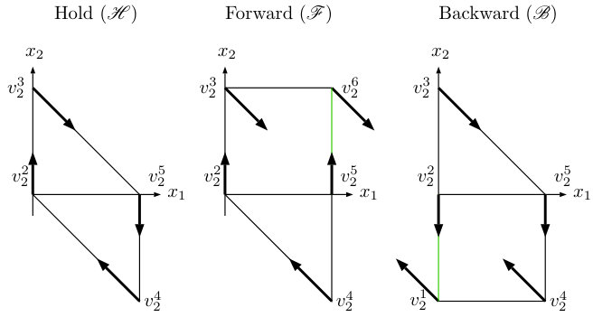 Figure 1
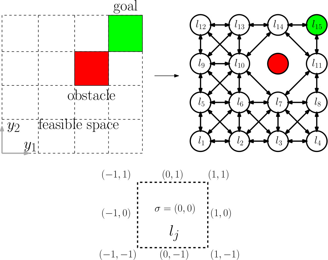 Figure 2
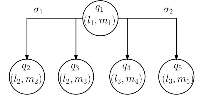 Figure 3
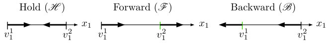 Figure 4
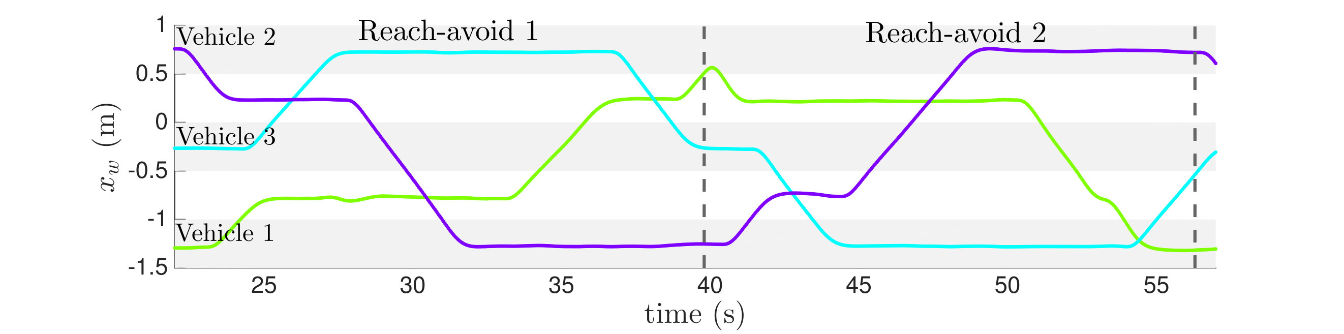 Figure 5
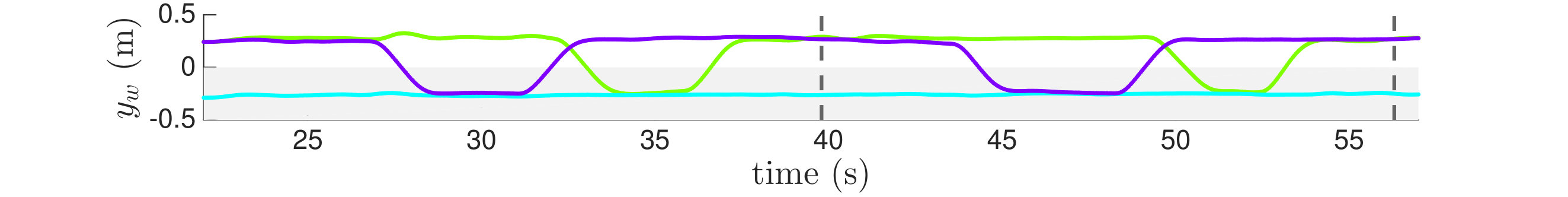 Figure 6
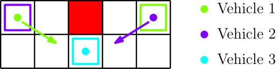 Figure 7
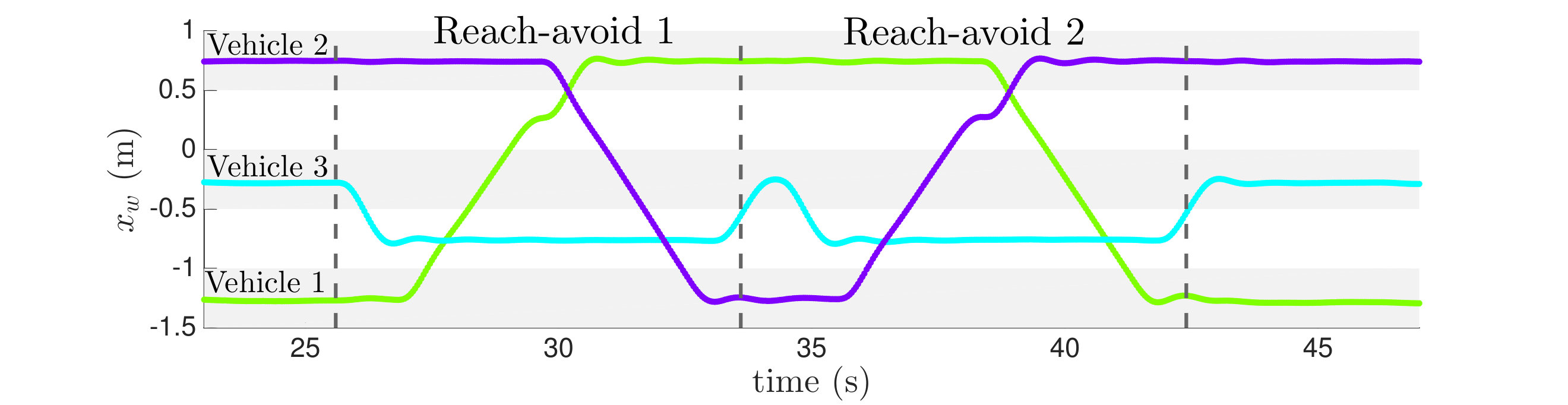 Figure 8
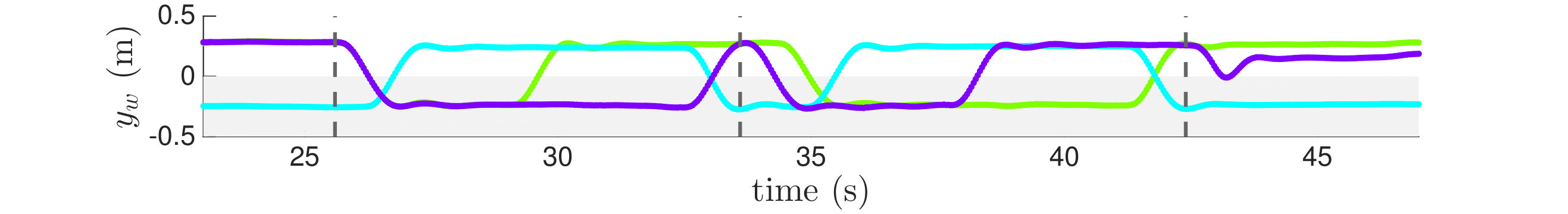 Figure 9
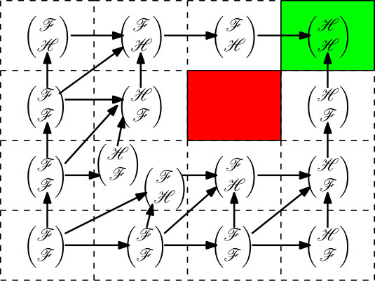 Figure 10
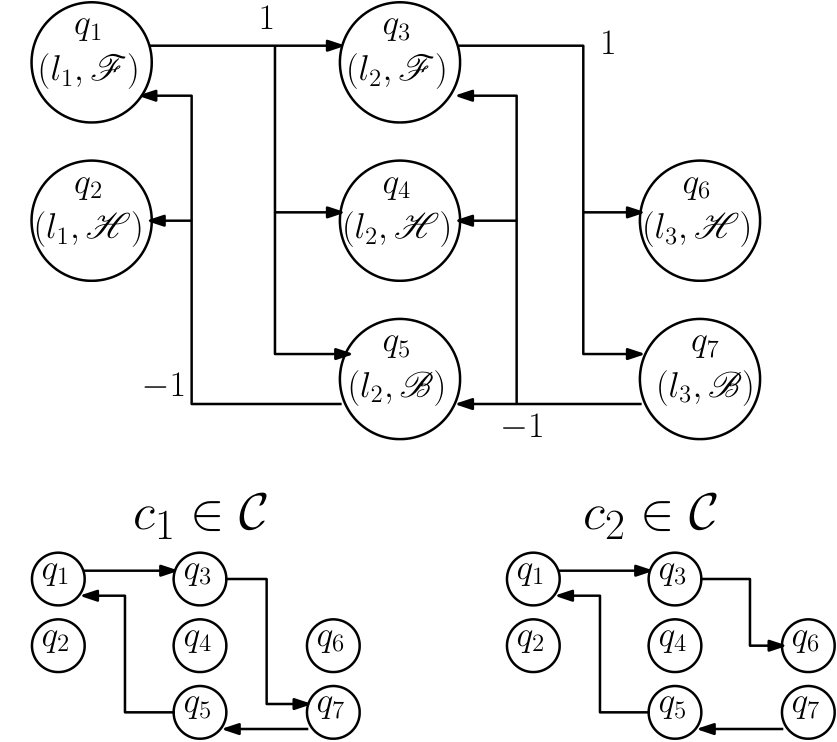 Figure 11
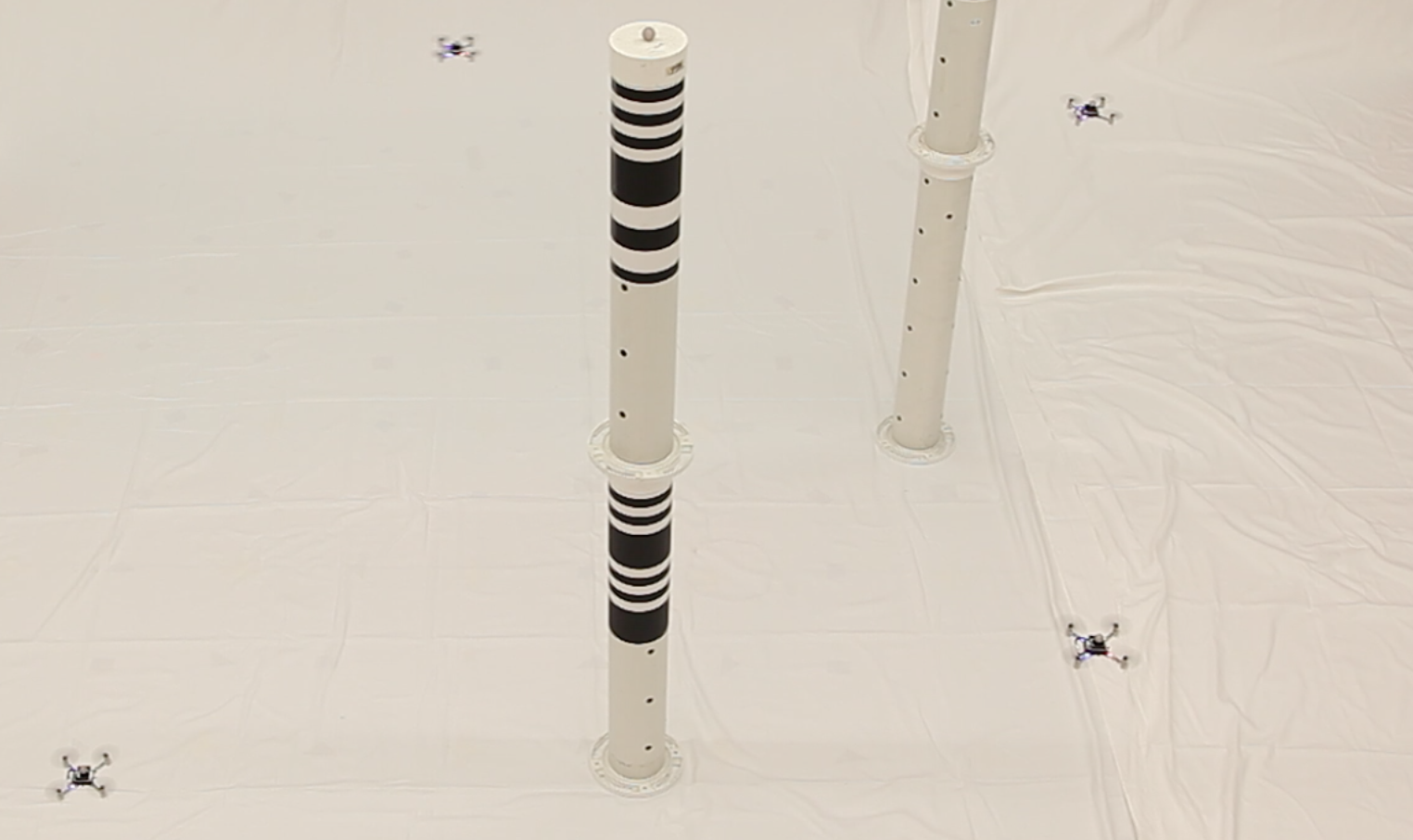 Figure 12
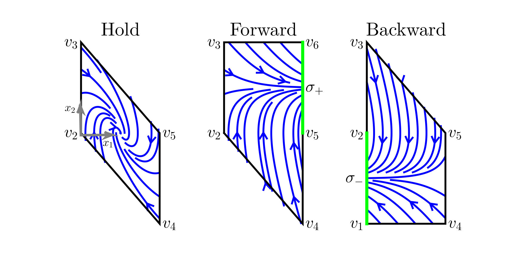 Figure 13
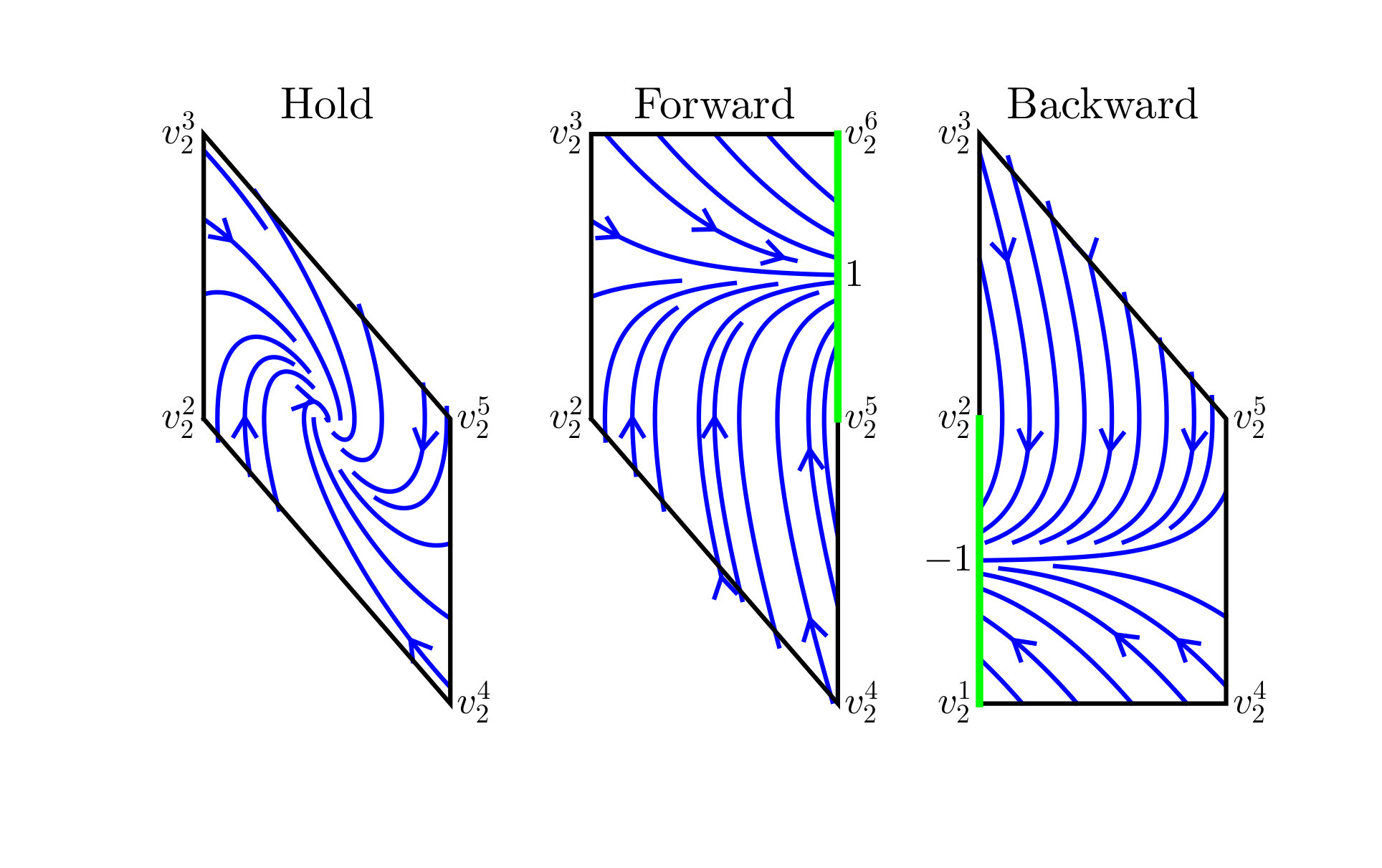 Figure 14
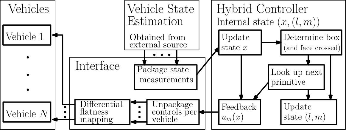 Figure 15
 Figure 16
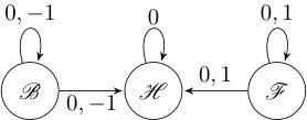 Figure 17
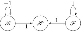 Figure 18
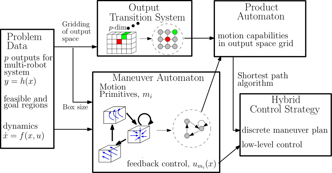 Figure 19
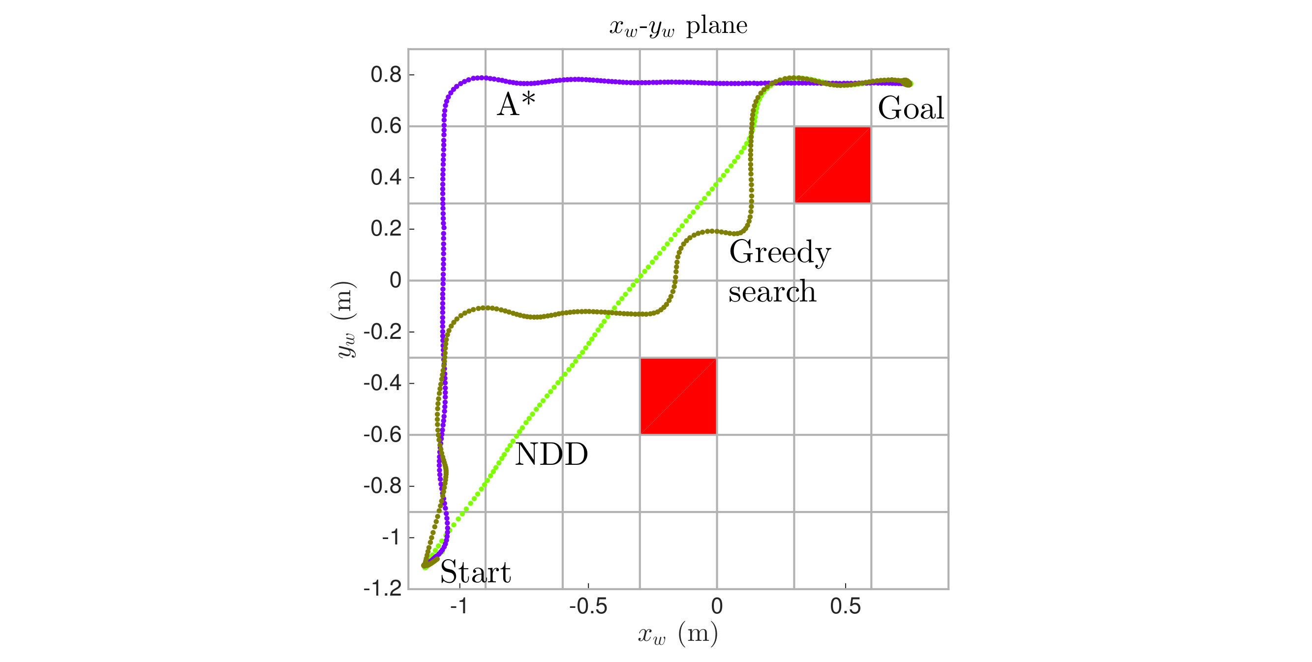 Figure 20
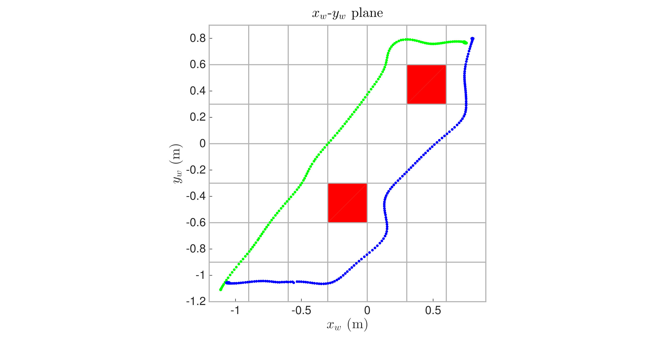 Figure 21
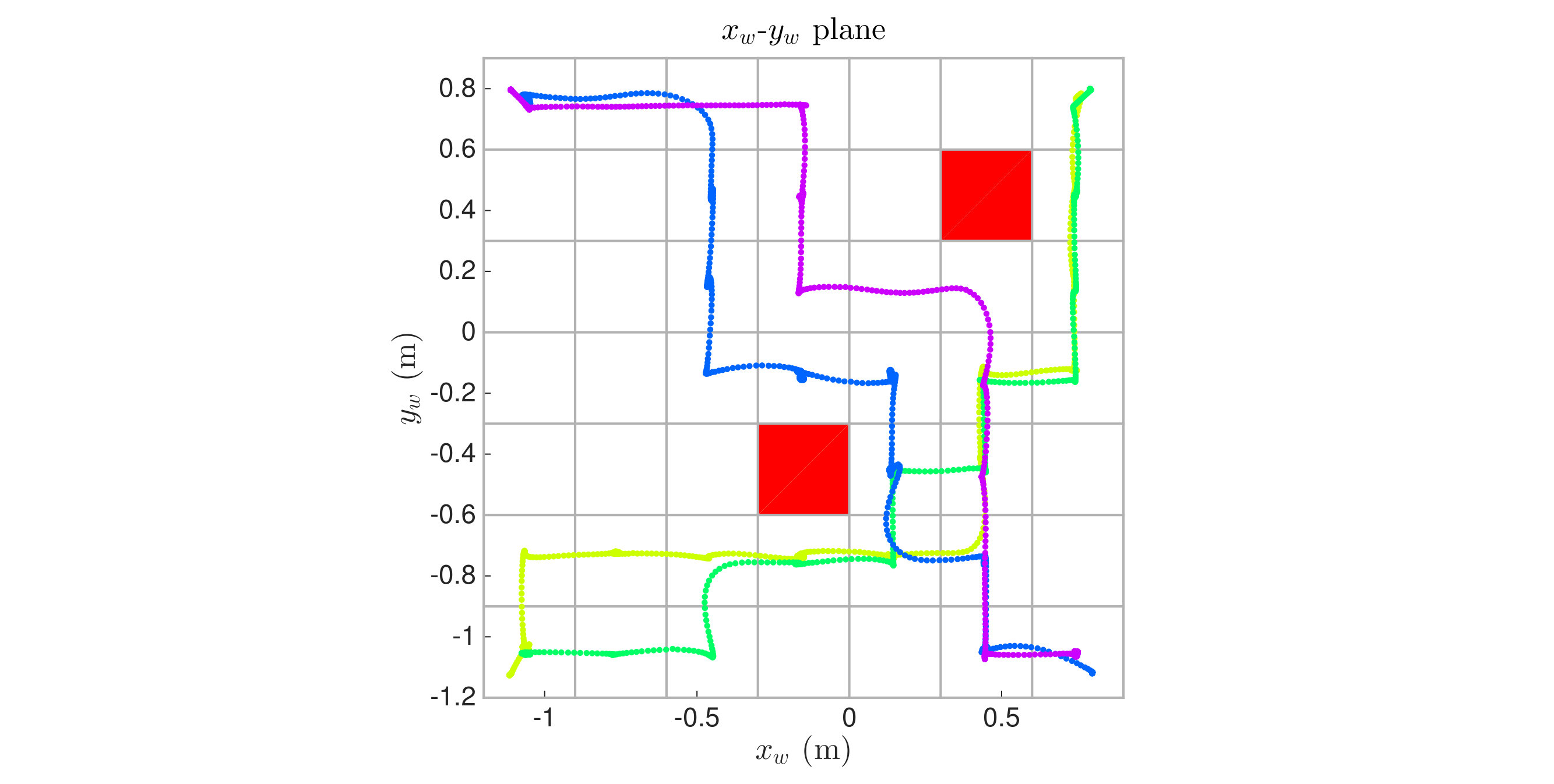 Figure 22
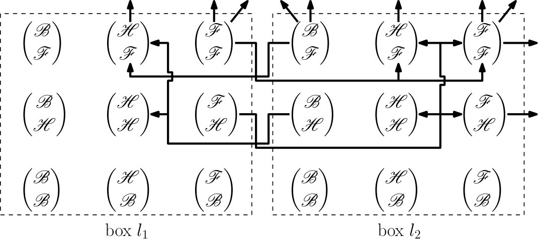 Figure 23
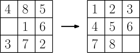 Figure 24
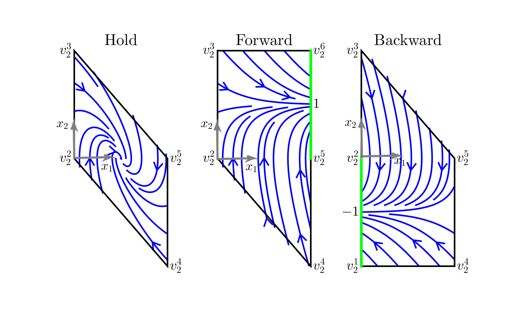 Figure 25
Peer Reviews
No public reviews on file for this paper yet. If you reviewed it on a platform where reviews are public (OpenReview, ICLR, NeurIPS, ICML), you can paste yours below so the community can read it here.
Videos
No videos yet. Explain this paper in a talk, walkthrough, or lecture? Add one.
Taxonomy
TopicsRobotic Path Planning Algorithms · Robot Manipulation and Learning · Formal Methods in Verification
A Modular Framework for Motion Planning using Safe-by-Design Motion Primitives
Marijan Vukosavljev, Zachary Kroeze, Angela P. Schoellig, and Mireille E. Broucke Marijan Vukosavljev, Zachary Kroeze, and Mireille E. Broucke are with the Dept. of Electrical and Computer Engineering, University of Toronto, Canada (e-mails: [email protected], [email protected], [email protected]). Angela P. Schoellig is with the University of Toronto Institute for Aerospace Studies (UTIAS), Canada (email: [email protected]). Supported by the Natural Sciences and Engineering Research Council of Canada (NSERC).
Abstract
We present a modular framework for solving a motion planning problem among a group of robots. The proposed framework utilizes a finite set of low level motion primitives to generate motions in a gridded workspace. The constraints on allowable sequences of motion primitives are formalized through a maneuver automaton. At the high level, a control policy determines which motion primitive is executed in each box of the gridded workspace. We state general conditions on motion primitives to obtain provably correct behavior so that a library of safe-by-design motion primitives can be designed. The overall framework yields a highly robust design by utilizing feedback strategies at both the low and high levels. We provide specific designs for motion primitives and control policies suitable for multi-robot motion planning; the modularity of our approach enables one to independently customize the designs of each of these components. Our approach is experimentally validated on a group of quadrocopters.
I Introduction
This paper presents a modular, hierarchical framework for motion planning and control of robotic systems. While motion planning has received a great deal of attention by many researchers, because the problem is highly complex especially when there are several robotic agents working together in a cluttered environment, significant challenges remain. Hierarchy, in which the control design has several layers, is an architectural strategy to overcome this complexity. Almost all hierarchical frameworks for motion planning aim to balance flexibility in the control specification at the high level, guarantees on correctness and safety at the low level, and computational feasibility overall.
Historically motion planning was focused on high level planning algorithms, while suppressing details on the dynamic capabilities of the robots at the low level [19]. Taking full account of low level dynamics in combination with solving the high level planning problem can lead to a computationally intractable problem. Despite the wealth of available research [9, 28, 3, 17], computationally efficient solutions to the motion planning problem with tight integration of high and low levels are highly sought after.
We propose a modular hierarchical framework so that one can independently plug and play both low level controllers and high level planning algorithms in order to realize a balance between flexibility at the high level, safety at the low level, and computational feasibility. To make a customizable approach feasible, we introduce three assumptions. First, the output space of the underlying dynamical system has translational symmetry, namely position invariance, a property satisfied by many robotic models [12]. Second, the output space is gridded uniformly into rectangular boxes. Finally, the control capabilities are discretized into a finite set of motion primitives, where the low level describes the implementation of the motion primitives while the high level selects the motion primitives. Together, these assumptions imply that motion primitives can be designed over a single box, so that they can then be reapplied to any other box.
Now we give an overview of the features and techniques we employ, and we highlight other frameworks that share those features. We provide general formulation of motion primitives for nonlinear systems so that they can be applied to multi-robot systems. We focus on reach-avoid specifications in a priori known environments, in which the system must reach a desired configuration in a safe manner [3, 9, 15, 20]. Reach-avoid offers a fairly rich behavior set so that, for instance, a fragment of linear temporal logic (LTL) can be encoded as a sequence of reach-avoid problems [33], as we also show in our applications.
As we have mentioned, we abstract the output space into rectangular regions [28] rather than more general polytopic regions [9, 11, 17, 20] in order to exploit symmetry. Motion primitives have been employed in various ways [28, 15] and we encode feasible sequences of motion primitives by a maneuver automaton [12]. In contrast to the motion primitive methods above, our implementation of the low-level control design of motion primitives is based on reach control theory[27, 4], which provides a highly flexible and intuitive set of design tools that have two notable advantages over tracking: first, it is not necessary to find feasible open-loop trajectories to track; second, safety constraints on the system states during the execution and concatenation of motion primitives can be guaranteed by design. Finally, planning at the high level is based on standard shortest path algorithms [19, 5] applied to the graph arising from the synchronous product of the discrete part of the maneuver automaton and the graph arising from the output space partition. The high-level plan generates a control policy, which selects the motion primitives over the gridded output space. The modularity of our approach enables one to employ other closed-loop methods such as potential methods [9] or vector-field shaping [20] for low-level control design, and standard or customized graph search algorithms to generate a high-level plan.
There are three main contributions of this work. First, we provide the complete theoretical details on the requirements for the low-level control design and high-level plan, and show that these two levels operate consistently to solve the reach-avoid problem. Second, we formulate the parallel composition of maneuver automata in order to obtain correct-by-design motion primitives for a system composed of individual subsystems, such as in the case of multiple vehicles. Finally, the modularity and effectiveness of our framework is experimentally validated on a group of quadrocopters in several illustrative scenarios. In particular, we feature a novel and versatile design of motion primitives based on double integrators and we show how the customizability of the high level plan generation can be used to easily trade-off solution quality with computational efficiency. This paper is an extension of our previous work [31], which now supplies all the theoretical details along with proofs on correctness, the parallel composition construction, additional approaches to generate control policies, and more elaborate experimental results.
The paper is organized as follows. In the next section we highlight our contributions relative to the literature. In Section III we present a formal problem statement. The modular framework is introduced in Section IV. We define the output transition system, the maneuver automaton, the product automaton, and the high level plan, each of which contribute to realizing a solution of the motion planning problem. In Section V, we prove that our overall methodology solves the motion planning problem. In Section VI we give the procedure for composing motion primitives. In Section VII we present specific motion primitives for a double integrator system. In Section VIII we consider several methods to generate high level plans, which are experimentally demonstrated on quadrocopters. We conclude the paper in Section IX.
Notation. Let denote the integers and denote the real numbers. Let denote the cardinality of a set. If is a set, we denote its power set as . If and are sets, let denote the usual set difference. If there are sets , let denote the usual cartesian product. Given a function , the image of under and the preimage of under are defined the usual way, and are denoted as and , respectively. Let denote the convex hull of the vectors . Given two vectors , we denote the component-wise multiplication (or Hadamard product) as . Let denote the set of globally Lipschitz vector fields on .
II Related Literature
The literature on motion planning is vast and encompasses many research communities. As such, we have categorized some common approaches and discussed how they relate to our method.
II-A Graph Search and Trajectory Planning
Motion planning has often been addressed as a discrete planning problem, for which many standard graph search algorithms exist [19]. Recent work on the multi-agent reach-avoid problem has developed novel algorithms in the context of applications such as manufacturing and warehouse automation, aiming to balance computational efficiency with solution quality. For example, a centralized approach is given in [35], discretizing the workspace into a lattice and using integer linear programming to minimize the total time for robots to traverse in high densities. In [10], a sampling-based roadmap is constructed in the joint robot space using individual robot roadmaps, which is shown to be asymptotically optimal. Prioritized planning enables to safely coordinate many vehicles and is considered in a centralized and decentralized fashion in [6]. Subdimensional expansion computes mainly decentrally, but coordinates in the joint search space when agents are neighboring [32]. While such approaches typically provide various theoretical guarantees on the proposed algorithms, dynamical models and application on real robotic systems is often not considered.
The modularity of our framework is complementary, as it potentially enables existing multi-agent literature on gridded workspaces to be used directly or adapted for the generation of a high-level plan when used in conjunction with our proposed formulation of motion primitives. However, the consideration of continuous time dynamics may complicate the application of discrete planning methods in two ways. First, we must contend with constraints on successive motion primitives so that the continuous time behavior is acceptable - for example, avoiding abrupt changes in velocity. Second, we must contend with non-deterministic transitions to neighboring boxes, because motion primitives may allow more than one next box to be reached [18] - for example, modeling the joint asynchronous motion capabilities of a multi-robot system.
Trajectory tracking methods have also been applied to the formation change problem on real vehicles with complex dynamics. A sequential convex programming approach is given in [2], which computes discretized, non-colliding positional trajectories for a modest number of quadrocopters. More recently, an impressive number of quadrocopters were coordinated in [25], by first computing a sequence of grid-based waypoints and then refining it into smoother piecewise polynomials. However, since these open-loop trajectories are computed offline, deviations from the computed trajectories could result in crashes. On the other hand, our approach is more robust as it is completely untimed, carefully monitoring the progress of vehicles over the grid in a reactive way based on the measured box transitions.
II-B Formal Methods
A growing body of research has explored the use of formal methods in motion planning. This paper has been particularly inspired by [17], which provides a general framework for solving control problems for affine systems with LTL specifications. Their approach involves constructing a transition system over a polyhedral partition of the state space that arises from linear inequality constraints that constitute the atomic propositions of the LTL specification. Transitions between states of the transition system can occur if there exists an affine or piecewise affine feedback steering all continuous time trajectories from one polyhedral region to a contiguous one. Similar works to [17] include [9, 14, 20], which consider the simpler reach-avoid problem. Single and multi-robot applications followed shortly after in [11] and [3] respectively.
The appeal of these approaches is derived from their generality and faithful account of the low level system capabilities. On the downside, these methods generally do not scale well to larger state space dimensions, and so they would have limited applicability to large multi-robot systems. Our approach specializes these ideas by exploiting symmetry in the system dynamics and grid partition in order to strike a better balance between generality and computational efficiency. In particular, our feedback controllers are given as motion primitives, which can be designed independently of the obstacle and goal locations.
More recent works have also built on these formal method approaches, investigating more complex and realistic multi-robot problems. For example, service requests by multiple car robots in a city-like environment with communication constraints was considered in [7]. A cooperative task for ground vehicles was addressed in a distributed manner, enabling knowledge sharing amongst neighbors and reconfiguration of the motion plan in real time [13]. Tasks such as picking up objects are considered in conjunction with motion requirements in [26]. Since these works consider only fairly simple vehicle dynamics, they place greater emphasis on the synthesis of discrete plans satisfying the task specification. On the other hand, this paper considers the simpler reach-avoid problem in order to develop a formulation of motion primitives for nonlinear systems with symmetries.
II-C Motion Primitives
The usage of motion primitives has become popular recently in robotics, as they serve to simplify the motion planning problem by using predefined executable motion segments. Many variations exist, which have designed motion primitives using timed reference trajectories to control a formation of quadrocopters [28], paths on a state space lattice for a mobile robots [24, 8], and funnels in the state space centered about a reference trajectory for a car [15] and a small airplane [22].
We have been inspired by ideas in [12], from which we borrowed the term “maneuver automaton”. They define a motion primitive either as an equivalence class of trajectories or a timed maneuver between two classes, whereas we define a motion primitive as a feedback controller over a polyhedral region in the state space. In our formulation, concatenations between motion primitives are possible only across contiguous boxes in the output space, which provides a strict safety guarantee during concatenation. Moreover, this enables our approach to simplify obstacle avoidance to a discrete planning problem over safe boxes as in [8], bypassing the need to concatenate motion primitive trajectories using numerical optimization techniques as in [12].
Our presentation of the maneuver automaton gives explicit constraints on the design of motion primitives so that they can used reliably for high level planning. We have also introduced the notion of parallel composition of maneuver automata to build motion primitives for multi-robot systems. While our construction resembles existing methods of parallel composition [34, 30], we additionally prove that our construction preserves desired properties that enable consistency between the low and high levels. To the authors’ best knowledge, this paper is the first rigorous treatment of feedback-based motion primitives defined on a uniformly gridded output space.
III Problem Statement
Consider the general nonlinear control system
[TABLE]
where is the state, is the input, and is the output. Let and denote the state and output trajectories of (1) starting at initial condition and under some open-loop or feedback control.
Let be a feasible set in the output space and let be a goal set. In multi-vehicle motion planning contexts, represents the feasible joint output configurations of the system, which can arise from specifications involving obstacle avoidance, collision avoidance, communication constraints, and others. We consider the following problem.
Problem III.1** (Reach-Avoid).**
We are given the system (1), a non-empty feasible set and a non-empty goal set . Find a feedback control and a set of initial conditions such that for each we have
- (i)
Avoid*: for all ,*
- (ii)
Reach*: there exists such that for all , .*
We make an assumption regarding the outputs of the system (1) in order to exploit symmetry; see [12] for an exposition on nonlinear control systems with symmetries.
Assumption III.1**.**
First, we assume that there is an injective map associating each output to a distinct state, so that . We define the (injective) insertion map as , which satisfies and for all . Second, we assume that the system has a translational invariance with respect to its outputs. That is, for all , and , we have .
The assumption that the outputs of the system are a subset of the states is used in our framework to be able to design feedback controllers in the full state space that achieve desirable behavior in the output space. The second statement says that the vector field is invariant to the value of the output. In the literature this condition is called a symmetry of the system or translational invariance. This assumption is satisfied for many robotic systems, for example, when the outputs are positions. Also, we will see in Section VII that it significantly simplifies our control design.
IV Modular Framework
In this section we present our methodology to solve the motion planning problem in the form of an architecture that breaks down Problem III.1. This architecture consists of five main modules, as depicted in Figure 2.
- •
The Problem Data include the system (1) with outputs satisfying Assumption III.1 and a reach-avoid task to be executed in the output space.
- •
The Output Transition System (OTS) is a directed graph whose nodes (called locations) represent -dimensional boxes on a gridded output space and whose edges describe which boxes in the output space are contiguous.
- •
The Maneuver Automaton (MA) is a hybrid system whose modes correspond to so-called motion primitives. Each motion primitive is associated with a closed-loop vector field by applying a feedback law to (1). The edges of the MA represent feasible successive motion primitives. Each motion primitive generates some desired behavior of the output trajectories of the closed-loop system over a box in the output space. Because of the uniform gridding of the output space into boxes and because of the symmetry in the outputs described in Assumption III.1, motion primitives can be designed over only one canonical box .
- •
The Product Automaton (PA) is a graph which is the synchronous product of the OTS and the discrete part of the MA. It represents the combined constraints on feasible motions in the output space and feasible successive motion primitives.
- •
The Hybrid Control Strategy is a combination of low level controllers obtained from the design of motion primitives, and a high level plan on the product automaton.
Next we describe in greater detail the OTS, MA, and PA.
IV-A Output Transition System
The OTS provides an abstract description of the workspace or output space associated with the system (1). It serves to capture the feasible motions of output trajectories of the system (1) in a gridded output space, as in Figure 3. Specifically, we partition the output space into -dimensional boxes with lengths , where is the length of -th edge. We use a finite number of boxes to under-approximate the feasible set . Enumerating the boxes as , the -th box can be expressed in the form , where , are constants. We require that . Among these boxes, we assume there is a non-empty set of indices , so that we may similarly under-approximate the goal region as . We define a canonical -dimensional box with edge lengths given by . Each box , is a translation of by an amount along the -th axis.
Definition IV.1**.**
Given the lengths and a non-empty goal index set , an output transition system (OTS) is a tuple with the following components:
State Space
* is a finite set of nodes called locations. Each location is associated with a safe box in the output space and hence we write .*
Labels
* is a finite set of labels. A label is used to identify the offset between neighbouring boxes.*
Edges
* is a set of directed edges where if , , and . Thus, for each , the neighbouring box is either one box to the left (), the same box (), or one box to the right (). In this manner records the offset between contiguous boxes.*
Final Condition
* denotes the set of locations associated with goal boxes.*
- *
Remark IV.1**.**
We observe that the OTS is deterministic. That is, for a given and , there is at most one such that . This follows immediately from the fact that records the offset between the neighbouring boxes.
Figure 3 shows a sample OTS for a simple scenario. The OTS locations are associated with 15 feasible boxes, including a goal box for the reach-avoid task. The OTS edges are shown as bidirectional arrows; for example, interpreting and on the grid, then .
IV-B Maneuver Automaton
The maneuver automaton (MA) is a hybrid system consisting of a finite automaton and continuous time dynamics in each discrete state. The discrete states of the finite automaton correspond to motion primitives, while transitions between discrete states correspond to the allowable transitions between motion primitives. The continuous time dynamics are given by closed-loop vector fields (1) with a control law designed based on reach control theory (any other feedback control design method can be used).
Before presenting the MA, we first explain how this module is used in the overall framework. To solve Problem III.1, we assign motion primitives to the boxes of the partitioned output space such that obstacle regions are avoided and the goal region is eventually reached. The discrete part of the MA encodes the constraints on successive motion primitives. Such constraints might arise from a non-chattering requirement, continuity requirement, or requirement on correct switching between regions of the state space. A dynamic programming algorithm for assignment of motion primitives on boxes is addressed in Section IV-D; the salient point about this algorithm at this stage is that it only uses the discrete part of the MA.
In contrast, the continuous time part of the MA is used both for simulation of the closed-loop dynamics to verify that the motion primitives are well designed, as well as for the implementation of the low level feedback in real-time. The motion primitives are defined only on the canonical box to simplify the design. This simplification is possible because of the translational symmetry provided by Assumption III.1 and the fact that each box is a translation of . In simulation, a given motion primitive can cause output trajectories to reach certain faces of . If a face is reached, the output trajectory is interpreted as being reset to the opposite face and another motion primitive is selected to be implemented over (of course, the real experimental output trajectories do not undergo resets but move continuously from box to box in the output space). The selection of the next motion primitive is constrained by a combination of the previous motion primitive and the face of that is reached. The discrete transitions in the MA encode these constraints.
Definition IV.2**.**
Consider the system (1) satisfying Assumption III.1 and the box with lengths . The maneuver automaton (MA) is a tuple , where
State Space
* is the hybrid state space, where is a finite set of nodes, each corresponding to a motion primitive.*
Labels
, the same labels used in the OTS.
Edges
* is a finite set of edges.*
Vector Fields
* is a function assigning a globally Lipschitz closed-loop vector field to each motion primitive . That is, for each , we have where is a feedback controller associated with .*
Invariants
* assigns a bounded invariant set to each . We impose that . The set defines the region on which the vector field is defined. Note that there is no requirement that the invariant is a closed set.*
Enabling Conditions
* assigns to each edge , a non-empty enabling or guard condition . We require that . We make an additional requirement that lies on a certain face of determined by the label . Defining the face associated with as*
[TABLE]
we require that also .
Reset Conditions
* assigns to each edge a reset map . We require that , where is the Hadamard product. This definition says that the -th output component is reset to the right face of , , if , reset to the left face if , and unchanged otherwise. Overall, resets of states are determined by the event and only affect the output coordinates in order to maintain output trajectories inside the canonical box .*
Initial Conditions
* is the set of initial conditions given by .*
- *
Example IV.1**.**
Suppose the system is a double integrator and the first state is the translationally invariant output . The box is simply a segment. Let , where Hold () stabilizes , Forward () increases , and Backward () decreases . Referring to Figure 4, if is the current motion primitive and reaches the right face of , then the event occurs and we may select or as the next motion primitive. To correctly implement the discrete evolution of the MA in the continuous state space, an invariant and feedback control must be associated with each motion primitive, while an enabling and reset condition must be associated with each edge; see Figure 5. Formal details are given in Section VII.
We now formulate assumptions on the motion primitives so that correct continuous time behavior is ensured at the low level for consistency with the high level. For each , define the set of possible events as
[TABLE]
Assumption IV.1**.**
- (i)
For all , .
- (ii)
For all such that and , .
- (iii)
For all such that and , if , then .
- (iv)
For all such that and , .
- (v)
For all , .
- (vi)
For all , if then for all and , .
- (vii)
For all , if , then for all there exist (a unique) and (a unique) such that for all and for all , and .
- *
Condition (i) disallows tautological chattering behavior that arises by erroneously interpreting continuous evolution of trajectories in the interior of as “discrete transitions” of the MA (see Section V for definitions). Condition (ii) imposes that guard sets are independent of the next motion primitive. Since guard sets arise as the set of exit points of closed-loop trajectories from under a given motion primitive, it is reasonable that these exit points should depend only on the current motion primitive , and not on the choice of next motion primitive. Condition (iii) imposes that all guard sets corresponding to different labels are non-overlapping. This ensures that when the continuous trajectory reaches a guard , then it is unambiguous which edge of the MA is taken next; namely . Conditions (v), (vi), and (vii) are placed to guarantee that the MA is non-blocking. These conditions are based on known results in the literature [21]; see Lemma V.1. In order for condition (vii) to make sense, there must exist a unique label and a unique time for an MA trajectory to reach a guard set. First, we have uniqueness of solutions since the vector fields are globally Lipschitz. Second, the unique MA trajectory can only reach one guard set by condition (iii); this in turn means there is a unique . Obviously there exists a unique time to reach the guard set. Conditions (vi) and (vii) work together to state that either all trajectories do not leave, or all trajectories do eventually leave. Referring to Figure 5, all closed-loop state trajectories within the invariant of reach the guard set shown in green on the right. For either choice of next feasible motion primitive, or , trajectories enter the next invariant on the left due to the reset. Finally, condition (iv) eliminates potential chattering Zeno behavior, see Remark V.1.
Remark IV.2**.**
We make several further observations about the MA.
(i) The MA is non-deterministic in the sense that given and , there may be multiple such that . The discrete part of the MA is non-deterministic in a second sense: for each , the cardinality of the set may be greater than one. The latter situation corresponds to the fact that for different initial conditions of the continuous part, the associated output trajectories can reach different guard sets. In essence, which guard is enabled is interpreted, at the high level, as an uncontrollable event [34]. Remark IV.3 further illustrates these two types of non-determinism in the case of the PA.
(ii) The set of events in the MA correspond to the same events in the OTS. This correspondence is used in the product automaton PA, described in the next section, to synchronize transitions in the MA with transitions in the OTS. The interpretation is that when a continuous trajectory of the MA (over the box ) undergoes a reset with the label , the associated continuous trajectory of (1) in the box enters a neighboring box with the offset . Obviously, this interpretation assumes that the vector of box lengths is the same in both OTS and MA.
IV-C Product Automaton
In this section we introduce the product automaton (PA). It is constructed as the synchronous product of the OTS and the discrete part of the MA, namely . The purpose of the PA is to merge the constraints on successive motion primitives with the constraints on transitions in the OTS in order to enforce feasible and safe motions. As such, it captures the overall feasible motions of the system – any high level plan must adhere to these feasible motions.
Definition IV.3**.**
We are given an OTS and an MA satisfying Assumption IV.1. We define the product automaton (PA) to be the tuple , where
State Space
* is a finite set of PA states. A PA state satisfies the following: if there exists and such that , then there exists such that . That is, if all faces that can be reached by motion primitive lead to a neighboring box of the box associated with location of the OTS.*
Labels
* is the same set of labels used by the OTS and the MA.*
Edges
* is a set of directed edges defined according to the following rule. Let , , and . If and , then .*
Final Condition
* is the set of final PA states.*
- *
Remark IV.3**.**
Formally an automaton is said to be non-deterministic if there exists a state with more than one outgoing edge with the same label. The PA is non-deterministic. First, consider a PA state . Because the MA allows for more than one feasible next motion primitive such that , the PA will also have multiple next PA states such that . Second, there can be multiple possible labels such that for some . Thus, the PA inherits the two types of non-determinism of the MA that we discussed in Remark IV.2. For example, consider the PA fragment in Figure 6. For the first type of non-determinism, observe that there are two PA edges and with the same label. For the second type, observe that there are two possible events from , each with its own set of PA edges. Note also some additional structure: since the OTS is deterministic, the box state is in both and , corresponding to the OTS edge .
IV-D High-Level Plan
In this section we formulate the notion of a control policy on the PA, which gives a rule for selecting subsequent PA states by choosing the next motion primitive. Informally, the objective of the high level plan is to produce a control policy and find a set of initial PA states such that a goal PA state is eventually reached. To this end, in this section we also develop a Dynamic Programming Principle (DPP) suitable for use on the PA. Because of the two types of non-determinism of the PA, existing algorithms cannot be applied directly [5, 33]. By adapting the algorithm in [5], we obtain two formulations of the DPP, one of which is more computationally efficient as it exploits certain structure in the PA; further details are provided in Remark IV.5.
First some notation will be useful. Recall from (2), given , is the set of all labels on outgoing edges starting at . Similarly, is the set of all labels on outgoing edges starting at . That is,
[TABLE]
Now we formalize the semantics of the PA. A state of the PA is a pair where is a location in the OTS and is a motion primitive. A run of is a finite or infinite sequence of states , with and for each , there exists such that . We define the length of a run to be ; for infinite runs is defined to be . We consider a subset of runs starting at that satisfy one further property. If the run is infinite, then if . Instead if the run is finite, then if and additionally, . It is the latter requirement – that the last PA state of a finite run may not have outgoing edges in the PA – which is of interest. The interpretation is that we regard the event labels between PA states as uncontrollable, so if any event is possible, then it must occur eventually. Thus without loss of generality, each run is the prefix of a run . Further elaboration is given in Remark IV.4 (ii).
Given and , the set of admissible motion primitives is
[TABLE]
More generally, given and , the set of admissible motion primitives at is
[TABLE]
Next we introduce the notion of a control policy. Given and , an admissible control assignment at is a vector
[TABLE]
where , or equivalently . Notice that is a vector whose dimension varies as a function of the cardinality of the set . An admissible control policy is a map that assigns an admissible control assignment at each . Thus, for each and , . The set of all admissible control policies is denoted by .
Consider an admissible control policy and a state . We denote the set of runs in induced by as . Formally, if , and for all and , . Similarly, we denote the subset of runs in that eventually reach a state in as . Formally, if there exists an integer such that . For , we define
[TABLE]
Next we define an instantaneous cost , which satisfies for all , and a terminal cost . Now consider the run with , , and . We define a cost-to-go by
[TABLE]
Remark IV.4**.**
There are several notable features of our formula for the cost-to-go.
(i) For a given , there may be multiple runs due to the (second, non-standard type of) non-determinism of the PA. As such, we assume the worst case and take the maximum over in the cost-to-go. Moreover, we require for a finite cost-to-go so that is well-defined and all runs starting at eventually reach .
(ii) We have assumed that finite runs must terminate on PA states that have no outgoing edges. Suppose we included in finite prefixes of (finite or infinite) runs. These necessarily would be finite runs with final PA states that have outgoing edges. Then if we take a finite or infinite run that eventually reaches a goal PA state, certain finite prefixes of that run may not yet have reached a goal PA state, and we would get and an infinite cost-to-go. This anomaly arises from creating an artificial situation in which not all runs starting at an initial PA state reach a goal PA state because we included (unsuccessful) finite prefixes of successful runs.
(iii) The cost-to-go function also accounts for infinite runs by using the variable to record the first time a goal PA state is reached and by taking the cost only over the associated prefix of the infinite run. Although our primary focus is on reach-avoid specifications, in which finite runs terminate on goal PA states with no outgoing edges, infinite runs allow us to extend our framework to a fragment of LTL where, for example, a goal PA state is reached always eventually; see Remark V.3 for further details.
Example IV.2**.**
Consider the PA shown at the top of Figure 7 corresponding to a single output system with the three motion primitives from Example IV.1 over three boxes . Suppose that for all and that for all .
First consider the feasible control policy with the control assignments: , , , and . The bottom left of Figure 7 shows how the control policy trims away possible edges in the PA. Now suppose that . Choosing the initial condition and under the assumption that we do not include finite runs that terminate at PA states with outgoing edges, we can see that consists of only the single infinite run . Even though this run is infinite, , , and . Similarly, we compute , , , and . In contrast, the feasible control policy shown on the bottom right of Figure 7 only contains finite runs.
Next we define the value function to be
[TABLE]
The value function satisfies a dynamic programming principle (DPP) that takes into account the non-determinacy of ; see [5] where a slightly different result is proved. The proof is found in the appendix.
Theorem IV.1**.**
Consider and suppose . Then satisfies
[TABLE]
where , , , and .
Notice that for all such that , (since there can be no paths to the goal). Also, for all , .
Remark IV.5**.**
In (3) of Theorem IV.1, it is shown that can be computed using the local information of instead of using all of . In (4), the result is taken one step further by showing that can be calculated using only for each . The benefit of (4) becomes clear when we compare the cardinality of the sets over which the minimizations occur. Given , let . In (3) the minimization is over , and therefore the cardinality of the minimization set is . In (4) the minimization is over for each , and therefore the cardinality of the set is . While both (3) and (4) can be used to compute , in general (4) will be more computationally efficient.
Corollary IV.1**.**
Consider the control policy such that for all , and
[TABLE]
where , and . Then is an optimal control policy such that for all , .
Figure 8 shows a possible control policy for the scenario in Figure 3. Since there are two outputs, we use the motion primitives from Example IV.1 in each output; formal details are given in Section VI. The control policy was hand-computed. Notice that different routes may be taken from the same product state depending on the face reached, but ultimately the control policy ensures that all paths lead to the goal.
V Main Results
In this section we present our main results on a solution to Problem III.1. Our final result combines the notion of a control policy at the high level with feedback controllers executing correct continuous time behavior at the low level. First, in accordance with the reach-avoid objective (see Remark IV.4 (iii)), we assume the existence of motion primitives that can stabilize trajectories within a given box, that is, there exists such that . We restrict the final PA states to be goal OTS states equipped with such motion primitives
[TABLE]
Now suppose we have an admissible control policy derived using Theorem IV.1 or otherwise with as above. We present a complete solution to Problem III.1 including an initial condition set , a feedback control , and conditions on the motion primitives so that the reach-avoid specifications of Problem III.1 are met.
First we specify the initial condition set . The set of feasible initial PA states is
[TABLE]
That is, a feasible initial PA state satisfies that every run (induced by the control policy) starting at the PA state eventually reaches a goal PA state.
Now consider a state . It can be used as an initial state of the system if there is some for which the state is both in the box and in the invariant of . Recall that for all and , if and only if . With this in mind, we define the set of initial states to be:
[TABLE]
Next we specify the feedback controllers to solve Problem III.1. Consider any . Then for all such that , we define the feedback
[TABLE]
This defines a family of feedback controllers parametrized by , the state of (1) and by the PA state . These feedbacks work in tandem with the control policy , which effectively determines the next feasible PA state . For example, suppose and suppose the label is measured. This event corresponds to for . Let and let be the unique location of the OTS such that . Then the next PA state is and the controller that is applied in the next location is .
The main result of the paper is the following.
Theorem V.1**.**
Consider the system (1) satisfying Assumption III.1, the non-empty feasible set , and the goal set . Let be the vector of box lengths such that the goal indices is non-empty. Consider an associated OTS , an MA satisfying Assumption IV.1, a PA with as in (5), and an admissible control policy . Then the initial condition set given in (7) and the feedback controllers (8) solve Problem III.1.
In the remainder of this section we prove Theorem V.1. We now give a roadmap for these results. The verification of correctness at the low level is broken down into two steps that we now describe. First, we show that the MA is non-blocking in Lemma V.1. The key requirements are summarized in Assumption IV.1. The non-blocking condition ensures that MA trajectories continually evolve in time and stay within the invariant regions. We also put conditions to avoid chattering in which two discrete transitions can occur in immediate succession. While physical systems never undergo infinite switching in finite time, if our model predictions diverge from reality, then we have no grounds to claim that Problem III.1 is indeed solved. Second, in Lemma V.2 we show that to each closed-loop trajectory of (1) under the feedback controllers (8) and a control policy , we can associate a unique execution of the MA (defined below) and run of the PA.
We begin by describing the semantics of the MA. These definitions are standard; see [21]. A state of the MA is a pair , where and . Trajectories of the MA are called executions and are defined over hybrid time domains that identify the time intervals when the trajectory of a hybrid system is in a fixed motion primitive . Precisely, a hybrid time domain of the MA is a finite or infinite sequence of intervals , such that
- (i)
, for all ,
- (ii)
if , then either or ,
- (iii)
, for all .
Definition V.1**.**
An execution of the MA is a collection such that
- (i)
the initial condition of the execution satisfies: .
- (ii)
the continuous evolution of the execution satisfies: for all with , then for all , is constant and , while for all , .
- (iii)
a discrete transition of the execution satisfies: for all , there exists such that , , and .
Given an execution , we associate to it the output trajectory of the MA given by (the subscript MA is included to avoid confusion with output trajectories of the physical system (1) which do not undergo resets). The execution time of an execution is defined as . An execution is called finite if is a finite sequence ending with a compact time interval. An execution is called infinite if either is an infinite sequence or if . Finally, an execution is called Zeno if it is infinite but .
Remark V.1**.**
There are two types of Zeno behavior. In one type that we call chattering, transitions are instantaneous. The second more subtle type is when the times between discrete transitions of the MA converge to zero, but the transitions are not instantaneous. Assumptions IV.1 (i) and (iv) ensure that we cannot have chattering. True Zeno behavior with convergent transition times is more difficult to identify in the setting when the MA is formed as a parallel composition. Fortunately, for our reach-avoid objective, the induced MA executions cannot be Zeno since there are a finite number of transitions by construction, see Lemma V.2.
Definition V.2**.**
The MA is non-blocking if for all , the set of all infinite executions of the MA with initial condition is non-empty.
Lemma V.1**.**
Under Assumption IV.1, the MA is non-blocking.
Proof.
Let . If , then by Assumption IV.1 (vi), is invariant, so the trajectory starting at remains in for all future time. Therefore, trivially, the MA is non-blocking for this initial condition. If , then by Assumption IV.1 (vii), remains in until it reaches a guard set. Additionally, by Assumption IV.1 (v), the trajectory is mapped under the reset into the next invariant. By Lemma 1 of [21], the MA is again non-blocking for this initial condition. Overall, the MA is non-blocking. ∎
The purpose of the Assumptions IV.1 is to guarantee consistency between low level continuous time behavior and the high level discrete plan. This consistency is formalized by way of a one-to-one correspondence between infinite MA executions and finite PA runs, both starting from the same initial condition. The proof is found in the appendix.
Lemma V.2**.**
Suppose we have an admissible control policy , and we have an MA satisfying Assumption IV.1. For each and there exist a unique infinite MA execution and a unique finite PA run .
Before we can prove Theorem V.1 we need one further preliminary result stating that because of the translational invariance of Assumption III.1, the continuous part of an MA execution has a unique correspondence to a closed-loop trajectory of the system (1). The proof is straightforward and is omitted.
Lemma V.3**.**
Let , , , and . Consider the trajectory of (1) with the feedback control . Also consider the MA trajectory with feedback control . For all such that ,
[TABLE]
Finally we are ready to prove Theorem V.1.
Proof of Theorem V.1.
We must show that (i) output trajectories of system (1) remain within , and (ii) output trajectories eventually reach and remain within the goal set . Let . Choose any such that . By Lemma V.2, we may associate a unique MA execution and a unique PA run to and . Denote the hybrid time domain as with for (with ) and . The last interval follows from the definition of (5), since and thus Assumption IV.1 (vi) implies that we must have that . As in the proof of Lemma V.2, denote the corresponding sequence of events as .
Using Lemma V.3 with , we have that . We claim that for all and ,
[TABLE]
Clearly the result is true for .
We derive two facts to assist in proving this claim. Recall that by definition of the OTS edges, we have that for all , . Furthermore, by rearranging, multiplying component-wise by , and taking the preimage , we have the first fact: for all that . Also by definition of the reset map and MA execution, we get the second fact: for all , .
Returning to (9), by induction we assume that it is true for and show that it is true for . Using the above facts and (9) for at yields
[TABLE]
Applying Lemma V.3 with at the new initial condition , we have that for and for all that (9) holds. When , the induction terminates and the claim is proven.
Using (9) and projecting to the output space we conclude that for all and , . Since all the boxes are contained in by construction, then for all we have (i). Moreover, since implies the goal box is contained in and , we have (ii). ∎
Remark V.2**.**
The above result does not depend on the method of construction of the admissible control policy , nor does it require the control policy to be optimal. This allows for different path planning techniques on the PA, as we show in Section VIII-B.
Remark V.3**.**
The extension to a sequence of reach-avoid problems is straightforward, following the idea in [33]. First, the reach property (ii) of Problem III.1 is relaxed to . Next, suppose there is a finite sequence of goals , . In contrast to (5), we set the final PA states to be for . Finally, one must design control policies with associated initial conditions (6) such that for . For , one may impose solutions to remain invariant or connect back to the first goal.
VI Parallel Composition of Motion Primitives
In this section we describe the operation of parallel composition of two maneuver automata. By repeated application of this operation, more complex higher-dimensional MA’s can be constructed by starting from simple low dimensional atomic motion primitives, such as those described in Section VII. The key challenge is to ensure that the resulting parallel composed MA satisfies Assumptions IV.1, if the two constituent MA’s do. This is proved in Theorem VI.1. First we give some preliminary definitions and we fix some notation, followed by the formal definition of parallel composition of MA’s.
We consider two independent systems
[TABLE]
where , , and for . We use superscripts to identify the distinct subsystems. Assume that each system satisfies Assumption III.1. That is, for , , . Associated with each system is the MA
[TABLE]
We additionally assume that and satisfy Assumption IV.1. Denote the canonical boxes in the respective output spaces as . The event sets labelling the faces of are . The empty strings are denoted as , , and the empty string is . Other sets are similarly denoted with a superscript to identify the system, such as the set of possible events for and the output indices . For the parallel composition we also require some extra notation. First, for and for each , define the invariant set minus all the guard sets
[TABLE]
Next, we need three sets: an augmented set of edges that includes a transition with the empty string, an augmented set of possible events for a motion primitive , and an augmented set of next feasible motion primitives. That is, for , we define
[TABLE]
We also define the products of these sets:
[TABLE]
Finally, the canonical box in the output space of the parallel composition is . We can now define the parallel composition of two MA’s.
Definition VI.1**.**
Consider two MA’s and each satisfying Assumption IV.1. The parallel composition is where
State Space
* with and .*
Labels
* with .*
Edges
, where if , , and . Observe that for all , .
Vector Fields
For all , . The state is , the control input is where , and the output is . The output map is , with for and for .
Invariants
For all , .
Enabling and Reset Conditions
Consider an edge , where , , , and for . If and , then we define
[TABLE]
Otherwise if , we have and , corresponding to their definitions in . Finally, we define and .
Initial Conditions
* is the set of initial conditions given by .*
- *
First, notice that for each and for each , the definition of automatically includes self-loop edges . We include such transitions with so that the parallel composition is properly constructed. For example, suppose a proper face of is crossed by the first system, but no proper face of is crossed by the second system. To correctly account for such possibilities, the overall transition for the composed MA must record the lack of crossing in by the empty string . Second, notice that we have allowed for additional edges with to allow for the possibility of switching to a different motion primitive over the same box if the invariants overlap and are not mapped immediately to a guard set, as can be observed by the definition of . Referring to Figure 8, an edge such as consists of and , which encodes a turn from Right to Up.
The main result is now stated; the proof is in the appendix.
Theorem VI.1**.**
We are given and , two MA’s that satisfy Assumption IV.1. The parallel composition defined above is an MA that also satisfies Assumption IV.1.
Remark VI.1**.**
We have defined the event set as , but the usual parallel composition of automata would have [34]. Given the interpretation of the event set as crossing faces of , the cartesian product is the more natural choice.
VII Motion Primitives for Integrator Systems
In this section we give the formal details for the MA consisting of the three motion primitives Hold (), Forward (), and Backward () introduced in Example IV.1. This design is able to be succinctly expressed within the MA formalism since the underlying double integrator system satisfies Assumption III.1. By exploiting the parallel composition construction from Section VI, the usefulness of this MA is demonstrated in the context of multi-robot systems in Section VIII.
Suppose the nonlinear control system is the double integrator system:
[TABLE]
where , , and the output is the position. Each motion primitive’s invariant region is a polytopic set in the state space defined as the convex hull of vertices , ; see Figure 5. The vertices are determined by the segment length , and a pre-specified maximum control value . Let . The vertices are , , , , , and . For each motion primitive , we define an affine feedback
[TABLE]
Our specific choices are , , , and . These controllers are derived using reach control theory [27, 4]. One first selects control values at the vertices of the polytopes so that trajectories remain in the invariant region (for the Hold primitive) or they exit the polytope through a certain facet and not through others. In particular, we have chosen all the control values at the vertices to have magnitude . Then the velocity vectors at the vertices are affinely extended to obtain affine feedbacks over the entire polytope, yielding the vector fields shown in Figure 5.
Now we construct the MA. The state space is . The labels are . The set of edges are shown in Figure 4. In the context of parallel composition, one may compute that the augmented edges are
[TABLE]
For each , the closed-loop vector fields are given by , which are clearly globally Lipschitz. The invariants are given by the convex hull of vertices, as seen in Figure 5, and excluding the two points and , so the invariants are clearly bounded. For example, . The enabling conditions are constructed by taking the convex hull of vertices of the exit facet and excluding again or . Specifically, the edges both have guard sets , as shown highlighted in green on the invariant region of in Figure 5, whereas both have guard sets . The reset conditions are constructed according to their definition. The proof of the following result is found in the appendix.
Lemma VII.1**.**
The double integrator MA satisfies Assumption IV.1.
Remark VII.1**.**
We noted in Remark V.1 that Zeno executions do not arise for reach-avoid specifications that, by construction, involve only finite MA executions. However, one may be interested in analyzing whether an MA is non-Zeno in its own right, independently of the high level plan or control specification for which it is used. It can be verified rather easily that the double integrator MA design we have presented above is non-Zeno. The situation is considerably more complicated when considering an MA that is a parallel composition of these MA’s or when considering an arbitrary MA. Generic conditions when hybrid systems have a Zeno execution have been studied in [16, 36]. However, further study of this problem is needed in our context since existing results do not apply to all the situations that can arise in our MA.
VIII Quadrocopter Applications
In this section we apply our methodology to a group of quadrocopters. We first explain how motion primitives can be applied to the system, how to specify the reach-avoid objective, and the overall solution pipeline. Next, we compare and contrast three algorithms for computing a control policy. Then we present experimental results on three different scenarios. Lastly, we provide a discussion.
VIII-A Interfacing Multiple Quadrocopters
The standard quadrotor dynamical model has six degrees of freedom, which can be described by the inertial linear positions and the roll-pitch-yaw Euler angles [25, 23]. It is well known that this system is differentially flat, relating the full state and motor inputs of the quadrotor to the flat outputs and their derivatives [23]. Rather than specifying positional reference trajectories, we use the motion primitives from Section VII independently in the directions to compute the linear accelerations as a feedback on the linear position and velocity states. Specifying an arbitrary yaw reference, differential flatness maps these linear accelerations to the angles and the total vehicle thrust, which through the use of an attitude tracking controller can be converted to motor inputs [23]. Although we have avoided computing motion primitives on the high dimensional nonlinear model, our experiments show that the quadrotor is fairly well approximated as double integrators in the directions using our proposed motion primitives.
We consider a centralized reach-avoid objective among quadrocopters. A copy of the gridded 3D workspace must be associated with each vehicle, resulting in a total of outputs. The -dimensional MA representing the asynchronous motion capabilities of the multi-vehicle system is obtained by parallel composing times the single-output MA from Section VII.
To specify the reach-avoid objective, we must identify the obstacle and goal boxes in dimensions. First we assume that the physical obstacles and goals for each vehicle are labelled on the physical 3D grid. Obstacle boxes in the output space correspond to any vehicle occupying a physical obstacle box or any two or more vehicles occupying the same physical box simultaneously. To avoid the effects of downwash, we do not allow vehicles to simultaneously occupy boxes that are displaced only in the direction. Goal boxes in the output space correspond to all the combinations of individual vehicle 3D goal boxes. For simplicity, we assume that each vehicle has a single 3D goal box.
The multi-vehicle reach-avoid problem is solved offline using our proposed methodology. The runtime workflow is depicted in Figure 9. Each runtime component requires negligible computation, even for a large number of vehicles and outputs.
VIII-B Control Policy Generation
We highlight three options for generating a control policy in the context of the multi-vehicle reach-avoid problem. For each, we give some implementation details and discuss its computational complexity. These are then compared in the experiments.
VIII-B1 Exhaustive Non-Deterministic Dijkstra (NDD)
The first strategy follows the proposed methodology of Section IV. We highlight our main implementation steps. First, we compute the OTS states and edges for the associated output space obstacle boxes described earlier. Second, the times parallel composed MA states and edges are computed. Third, the PA states and edges are computed. Fourth, the value function is computed using (4). This is done by initializing the value function to be zero at goal states and infinite elsewhere, and then propagating backwards along PA edges using a non-deterministic Dijkstra (NDD) algorithm [5, 33]. Once the value function is computed at all states, we compute the optimal control policy using Corollary IV.1. The initial PA states (6) correspond precisely to those states with .
The computational complexity grows exponentially as the number of inputs increases. Suppose that the physical grid has boxes in the directions. Since there are motion primitives, the number of PA states is bounded by . The number of edges from an OTS state is bounded by (the neighboring directions), whereas the number of edges from a MA state is bounded by (the neighboring directions times the possible next motion primitives). Since the MA neighboring directions are more restrictive, we have the number of PA edges is bounded by . The presence of obstacles can dramatically reduce the number of PA states and edges. The NDD algorithm generally must inspect all the PA states and edges to compute the value function. As a result, it is optimal and complete (with respect to the selected grid resolution and motion primitive capabilities), which results in the largest possible set of initial conditions .
VIII-B2 Deterministic
In this strategy, we make two simplifying assumptions to compromise the quality of the control policy in exchange for better computational efficiency. First, we take the times composed MA and prune out motion primitives enabling simultaneous motion. Second, we forego computing the largest possible set of initial conditions and instead assume that a single physical initial box is specified for each vehicle. As such, it is sufficient to compute a single path of boxes in the OTS connecting the initial and goal boxes in the dimensional output space. From this path the control policy is immediately extracted, by assigning to each box the unique motion primitive leading to the next neighboring box along the path. The path is computed using a standard algorithm [19], which starts from the initial box and propagates outwards until the goal box is reached. The (admissible) heuristic function is chosen to be the Manhattan distance, which is the sum of distances along each output direction from the current box to the goal box.
The number of nodes that must investigate is bounded by the maximum number of OTS boxes, , which still has exponential complexity in the number of robots. The pruned MA has motion primitives, corresponding to or in a single output component with elsewhere, plus the motion primitive . Thus from the current box, we must check the neighboring directions to select a feasible direction, taking into account out-of-bounds and obstacle configurations. In this implementation, the OTS, MA, and PA serve more as conceptual constructs, and do not need to be precomputed explicitly as it is expensive. In the worst case, the algorithm may investigate all boxes; as a result, it also produces a control policy that is complete with respect to the chosen grid and pruned MA motion capabilities. The policy produced by is of minimal length, but may have a long runtime execution.
VIII-B3 Deterministic Greedy Search
This strategy also makes use of the two simplifying assumptions as with above, but differs in how the path is constructed. In greedy (best first) search [19], the path is constructed by starting from the initial box in the output space and then extending it from the current box into any feasible neighboring direction that decreases the Manhattan distance to the goal box. Greedy search can often find a path very quickly, although not necessarily an optimal one. Moreover, since greedy search may fail to find a path, it is not complete.
VIII-C Experimental Results
Our experimental platform is the Crazyflie 2.0; see Figure 1. We used a VICON motion capture system to obtain the state estimates of the vehicles. Our implementation was done in Python 2.7.10 and ROS Kinetic, and computations were performed on a 64-bit Lenovo ThinkPad with an 8 core 3.0 GHz Intel Xeon processor and 15.4 GiB RAM. We illustrate three different scenarios and consider the three policy generation strategies on each of them. The corresponding video results are available at http://tiny.cc/modular-3alg.
VIII-C1 Open Space
The first representative scenario involves an open 3D space partitioned into a grid and a sparse collection of pillar-shaped obstacles. The left plot of Figure 10 compares the resulting 3D trajectories in the plane for the three strategies in the case of a single vehicle. The computation times were 40.63 milliseconds, 1.59 milliseconds, and 0.27 milliseconds for NDD, , and greedy search, respectively. The NDD algorithm offers the best quality control policy in that there is simultaneous motion in the different degrees of freedom whenever possible and the same policy can be used from any starting box. The and greedy search algorithms offer similar results to each other, with both producing an optimal path of length 14. Both yield less efficient grid-like motion that is defined only along a single path from the initial box, although a new policy can quickly be recomputed from different starting boxes. Based on simulation tests for a single vehicle, each of these algorithms scale well to larger spaces or finer grids; even NDD is able to compute a solution on a grid in about two minutes in the worst cases. Next we compare each strategy on more vehicles.
The middle plot of Figure 10 shows the resulting trajectories for two vehicles using NDD. The control policy was computed in about 18 minutes and is defined on about PA 180000 states. While the resulting control policy yields highly efficient motion defined over a large set of initial conditions, adding more vehicles or more boxes generally explodes the computation time and memory requirements. Thus NDD is best suited for small scenarios involving a modest number of vehicles, when one can afford to spend time precomputing the control policy.
The right plot of Figure 10 shows the resulting trajectories for four vehicles swapping corners of the room using greedy search. Since the vehicles and physical obstacles occupy a single box, greedy search performs well, as each action typically results in one vehicle making progress towards the goal. The computation time was about four milliseconds. Simulation results on a grid with eight vehicles placed randomly demonstrate that greedy search is usually able to find a solution on the order of one second. As one would expect, greedy search typically fails to find a solution if long wall-like or non-convex obstacles are introduced, or if the goals are not spaced out sufficiently. Furthermore, the time to execute the entire maneuver scales with the number of vehicles.
Finally we consider the deterministic algorithm. Although the resulting trajectories follow a path of optimal length, they look quite similar to those found by greedy search and thus are not shown. Moreover, the method quickly becomes more computationally expensive beyond three vehicles.
VIII-C2 Channel Swapping
The second representative scenario involves two rooms connected by a channel, defined over a grid, see Figure 11. Two of the vehicles must continually swap places, while the third is required to act as a gatekeeper. We specify this objective as an infinitely looping sequence of two distinct reach-avoid problems. This illustrates that reach-avoid is a useful building block for addressing more complex specifications.
The NDD algorithm produced both control policies in about 10 seconds, while the algorithm took about 0.03 seconds. Greedy search fails to find a solution because it is unable to coordinate the third vehicle away from its goal to make space for the other two. Since the resulting trajectories overlap in physical space, Figure 12 shows the trajectories as a function of time using the policy computed with NDD. The trajectories are highly non-trivial, but show that the objective is satisfied for at least one cycle of both reach-avoids. Although not shown, the trajectories computed using are similar but take a few seconds longer to execute the objective since the motion primitives are deterministic.
VIII-C3 8-Puzzle
We conclude our experimental results with the well-known 8-puzzle. On a grid, eight vehicles are placed randomly and must return to an ordered configuration, see Figure 13. For this application, the algorithm is the most suitable, computing the control policy in 0.32 seconds. The NDD approach would spend too much time precomputing edges in the high dimensional output space, while greedy search would never make progress. Results are available to view in the video.
VIII-D Discussion
Throughout the various experimental scenarios presented, we have demonstrated the modularity offered by our approach. The designer can customize their own algorithms for generating a control policy in order to trade-off solution quality with computational efficiency. Depending on the specific application scenario, a different control policy generation strategy may be more suitable.
In our analysis, all of the complexity was associated with the generation of the control policy for a given MA. The MA formalism enables us to generate control policies with no further regard to the continuous time trajectories that may result, due to the guarantees on discrete behavior encoded in the MA edges. On the other hand, the generation of a MA for an arbitrary system is a difficult challenge in its own right and is left to the discretion of the designer, although the design we have presented in Section VII can potentially be applied to control systems that are feedback-linearizable into a collection of double integrators. Taking care that the outputs are translationally invariant and that obstacle boxes can be computed, this includes end effector control of fully actuated robotic manipulators [29] and some wheeled vehicles through the use of look-ahead points [1].
Our approach offers robustness through the use of feedback-based motion primitives, as the construction of invariant regions ensures a wide range of initial conditions for which output trajectories exit through appropriate guard sets into subsequent boxes. Since the motion primitives are updated during execution based on the measured box transitions and control policy, we do not require timing estimates for completing box transitions, which can be difficult to compute. These features are advantageous under model uncertainty, which we must contend with since we base our motion primitive design on the double integrator model rather than the more complex quadrocopter model, and since aerodynamic effects arise when multiple quadrocopters fly in close proximity. Our previous work also demonstrated similar robustness of operation under wind disturbances generated by a fan on a larger quadrocopter [31]. Finally, we note that our framework can easily be applied to a heterogeneous team of robots; if each vehicle has its own MA, the parallel composition automatically constructs the overall MA for the multi-vehicle system.
Of course, our solution to Problem III.1 is conservative because we have restricted ourselves to a particular discretization, namely the choice of a partition into boxes and the use of motion primitives. As we have demonstrated, this is a reasonable trade-off, especially since the resolution of the output space discretization, the richness of motion primitives, and the complexity of the control policy are all design parameters.
IX Conclusion
We have developed a modular, hierarchical framework for motion planning of multiple robots in known environments. It consists of several modules. An output transition system (OTS) models the allowable motions of the robots by partitioning their workspace into boxes. A set of motion primitives is designed based on reach control on polytopes. A maneuver automaton (MA) captures constraints on successive motion primitives. Finally, a control policy is generated based on the synchronous product of the OTS and the discrete part of the MA. Overall we obtain a two-level control design which is highly robust, modular, and conceptually elegant. We presented a specific maneuver automaton for the double integrator system, and we showed how this design can be composed to obtain maneuver automata for multi-robot systems. The methodology was experimentally validated on a group of quadrocopters. Future work includes application of our methodology to different vehicle classes such as robotic manipulators or wheeled vehicles, and integration with more advanced multi-robot planning algorithms in dynamic environments.
The reference list from the paper itself. Each links out to its DOI / PubMed record.
- 1[1] B. d’Andrea-Novel, G. Bastin, and G. Campion. “Modelling and control of non-holonomic wheeled mobile robots”. International Conference on Robotics and Automation , 1991.
- 2[2] F. Augugliaro, A. P. Schoellig, and R. D’Andrea. “Generation of collision-free trajectories for a quadrocopter fleet: A sequential convex programming approach”. International Conference on Intelligent Robots and Systems , 2012.
- 3[3] N. Ayanian and V. Kumar. “Decentralized feedback controllers for multiagent teams in environments with obstacles”. IEEE Transactions on Robotics . Vol. 26, no. 5, pp. 878-887, 2010.
- 4[4] M.E. Broucke and M. Ganness. “Reach control on simplices by piecewise affine feedback”. SIAM J. Control and Optimization . Vol. 52, no. 5, pp. 3261-3286, 2014.
- 5[5] M. E. Broucke, S. Di Gennaro, M. Di Benedetto, and A. Sangiovanni-Vincentelli. “Efficient solution of optimal control problems using hybrid systems”. SIAM Journal on Control and Optimization , Vol. 43, no. 6, pp. 1923-1952, 2005.
- 6[6] M. C̆áp, P. Novák, A. Kleiner, and M. Selecký. “Prioritized planning algorithms for trajectory coordination of robots”. IEEE Transactions on Automation Science and Engineering , Vol. 12, no. 3, pp. 835-849, 2015.
- 7[7] Y. Chen, X. C. Ding, A. Stefanescu, and C. Belta. “Formal approach to the deployment of distributed robotic teams”. IEEE Transactions on Robotics , Vol. 28, no. 1, pp. 158-171, 2012.
- 8[8] M. Cirillo, T. Uras, and S. Koenig. “A lattice-based approach to multi-robot motion planning for non-holonomic vehicles”. International Conference on Intelligent Robots and Systems , 2014.