SmartTrack: Efficient Predictive Race Detection
Jake Roemer, Kaan Gen\c{c}, Michael D. Bond

TL;DR
SmartTrack is an optimized predictive race detection algorithm that improves detection accuracy over FastTrack while maintaining comparable performance, by introducing novel and existing optimizations.
Contribution
It introduces a new optimized predictive race detection algorithm, combining existing and novel techniques for improved performance and accuracy.
Findings
SmartTrack detects more data races than FastTrack.
SmartTrack achieves performance comparable to FastTrack.
The algorithm incorporates novel conflicting critical section optimizations.
Abstract
Widely used data race detectors, including the state-of-the-art FastTrack algorithm, incur performance costs that are acceptable for regular in-house testing, but miss races detectable from the analyzed execution. Predictive analyses detect more data races in an analyzed execution than FastTrack detects, but at significantly higher performance cost. This paper presents SmartTrack, an algorithm that optimizes predictive race detection analyses, including two analyses from prior work and a new analysis introduced in this paper. SmartTrack's algorithm incorporates two main optimizations: (1) epoch and ownership optimizations from prior work, applied to predictive analysis for the first time; and (2) novel conflicting critical section optimizations introduced by this paper. Our evaluation shows that SmartTrack achieves performance competitive with FastTrack-a qualitative improvement in…
Click any figure to enlarge with its caption.
 Figure 1
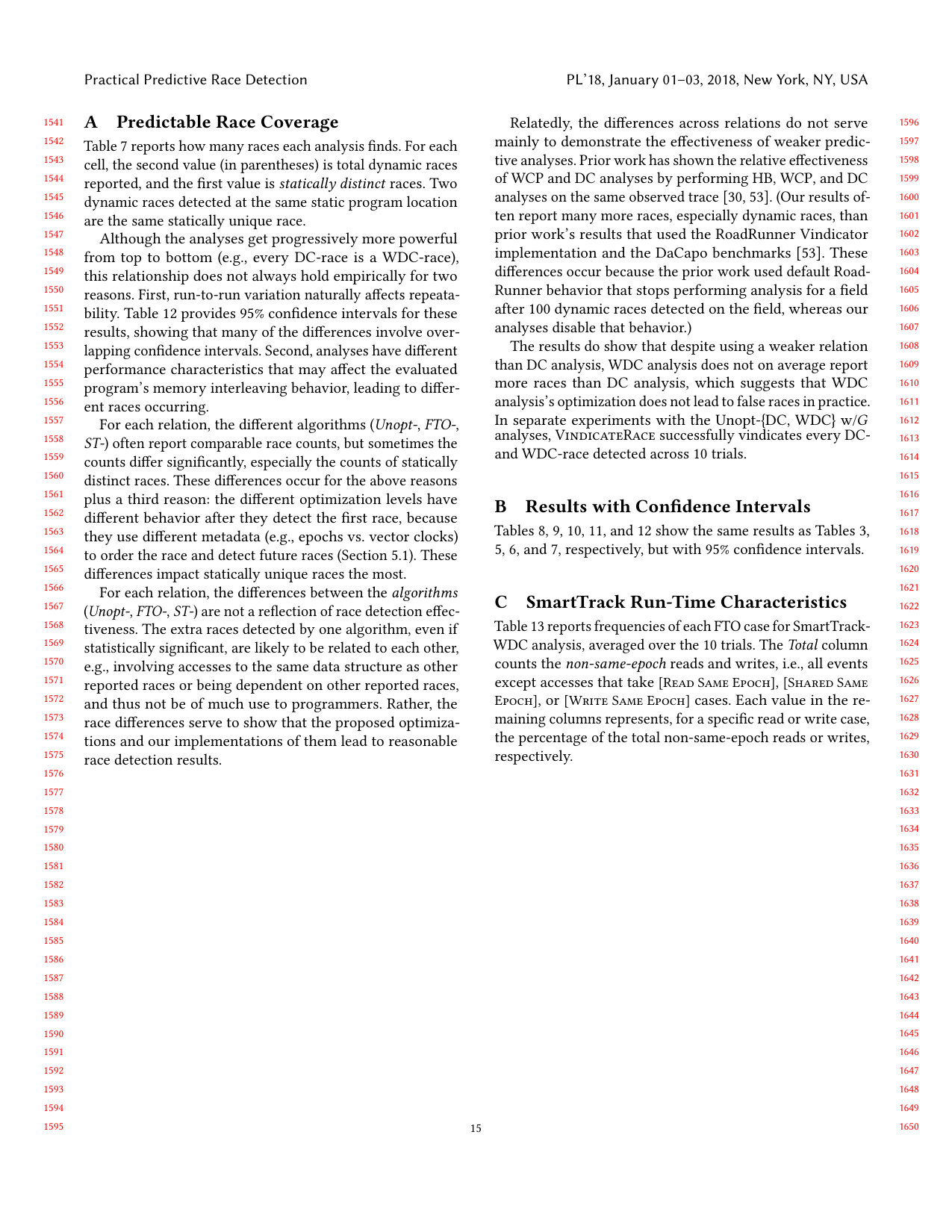 Figure 2
| Source of poor performance | Contribution | Speedup | |
|---|---|---|---|
| Release–release ordering | WDC relation and analysis | 1.04–1.25 | |
| Frequent vector clock operations | Epoch and ownership optimizations | } SmartTrack | 2.15–2.62 |
| Detecting conflicting critical sections (CCSs) | CCS optimizations | 1.51–1.74 |
| Prior work | This work | ||
| Non-predictive analysis: HB | 6.3 (4.9) | — | |
| Predictive analysis { | WCP | 34 (47) | 8.3 (7.5) |
| DC | 28 (32) | 8.6 (7.6) | |
| WDC | — | 6.9 (6.2) | |
| Unopt | Epochs | + Ownership | + CS optimizations | ||
| HB | Unopt-HB | FastTrack2 (Flanagan and Freund, 2017) | FTO-HB (Wood et al., 2017) | N/A | |
| WCP | Unopt-WCP (Kini et al., 2017) | — | FTO-WCP | SmartTrack-WCP | |
| DC | Unopt-DC (Algorithm 1) | — | FTO-DC (Algorithm 2) | SmartTrack-DC (Algorithm 3) | |
| WDC | Unopt-WDC | — | FTO-WDC | SmartTrack-WDC |
| Size | Events | Locks held at NSEAs | “Ancillary” metadata | Run time | Memory usage | |||||||||
|---|---|---|---|---|---|---|---|---|---|---|---|---|---|---|
| Program | #Thr | (LoC) | All | NSEAs | Check | Use | FT2 | FTO-HB | FT2 | FTO-HB | ||||
| avrora | 7 | 69 K | 1,400M | 140M | 5.9% | <0.1% | 0 | 6.8% | 0 | 5.3 | 5.4 | 13 | 13 | |
| batik | 7 | 188 K | 160M | 5.8M | 46.1% | <0.1% | <0.1% | 0 | 0 | 4.2 | 4.2 | 4.9 | 4.9 | |
| h2 | 16 | 116 K | 3,800M | 300M | 82.8% | 80.1% | 0.17% | 0.46% | <0.001% | 9.5 | 9.3 | 3.0 | 3.0 | |
| jython | 2 | 212 K | 730M | 170M | 3.8% | 0.23% | <0.1% | 0 | 0 | 8.3 | 8.3 | 7.0 | 7.0 | |
| luindex | 3 | 126 K | 400M | 41M | 25.8% | 25.4% | 25.3% | 0 | 0 | 7.9 | 8.0 | 4.3 | 4.3 | |
| lusearch | 16 | 126 K | 1,400M | 140M | 3.8% | 0.39% | <0.1% | <0.001% | 0 | 11 | 12 | 9.7 | 10 | |
| pmd | 15 | 61 K | 210M | 8.0M | 1.1% | 0 | 0 | 0 | 0 | 6.5 | 6.6 | 2.9 | 2.7 | |
| sunflow | 29 | 22 K | 9,700M | 3.5M | 0.78% | <0.1% | 0 | 0 | 0 | 17 | 17 | 8.4 | 8.4 | |
| tomcat | 55 | 159 K | 44M | 9.7M | 13.1% | 8.0% | 3.9% | 0.13% | <0.001% | 20 | 19 | 55 | 61 | |
| xalan | 15 | 176 K | 630M | 240M | 99.9% | 99.7% | 1.1% | 6.5% | 0 | 4.1 | 4.4 | 6.3 | 6.3 | |
| Unopt- | FTO- | SmartTrack- | ||
| HB | 19 | 6.3 | N/A | |
| WCP | 34 | 13 | 8.3 | |
| DC | 28 | 13 | 8.6 | |
| WDC | 27 | 12 | 6.9 | |
| Run time | ||||
| Unopt- | FTO- | ST- | ||
| HB | 6 (522,985) | 6 (407,783) | N/A | |
| WCP | 5 (552,479) | 6 (404,826) | 6 (406,667) | |
| DC | 5 (557,009) | 6 (404,260) | 6 (407,104) | |
| WDC | 5 (543,173) | 6 (406,348) | 6 (408,677) | |
| avrora | ||||
| HB | Unopt-DC | Unopt-WDC | |||||||
| Program | FT2 | FTO | w/ | w/o | w/ | w/o | |||
| avrora | 4.0 0.079 | 3.9 0.085 | 24 0.66 | 21 0.23 | 22 2.0 | 18 0.13 | |||
| batik | 4.1 0.065 | 4.0 0.077 | 11 0.55 | 10 0.41 | 11 0.46 | 10 0.37 | |||
| h2 | 8.3 0.11 | 8.3 0.13 | 79 5.2 | 85 6.0 | 80 1.5 | 89 1.7 | |||
| jython | 7.8 0.30 | 7.7 0.24 | 31 1.8 | 25 1.2 | 27 1.8 | 22 1.4 | |||
| luindex | 6.9 0.53 | 6.9 0.40 | 41 0.13 | 36 2.4 | 39 2.4 | 36 4.6 | |||
| lusearch | 9.8 0.92 | 9.8 0.73 | 28 2.6 | 26 0.25 | 26 0.59 | 29 11 | |||
| pmd | 6.3 0.21 | 6.4 0.21 | 17 2.1 | 16 1.6 | 15 14 | 15 1.4 | |||
| sunflow | 15 1.5 | 14 1.3 | 74 69 | 70 5.1 | 74 69 | 69 7.4 | |||
| tomcat | 4.2 0.14 | 4.0 0.16 | 15 0.11 | 17 0.94 | 9.8 0.26 | 12 1.4 | |||
| xalan | 4.0 0.33 | 4.0 0.34 | 54 55 | 45 2.4 | 48 49 | 39 5.1 | |||
| geomean | 6.4 | 6.3 | 31 | 28 | 28 | 27 | |||
| Run time | |||||||||
| Unopt- | FTO- | ST- | ||
| HB | 17 1.2 | 3.9 0.085 | N/A | |
| WCP | 23 0.54 | 7.8 0.14 | 5.9 0.064 | |
| DC | 21 0.23 | 8.0 0.12 | 6.4 0.11 | |
| WDC | 18 0.13 | 6.1 0.13 | 4.5 0.072 | |
| avrora | ||||
| Unopt- | FTO- | ST- | ||
| HB | 32 0.021 | 4.1 0.15 | N/A | |
| WCP | 99 0.60 | 11 0.36 | 7.2 0.26 | |
| DC | 42 0.13 | 11 0.34 | 7.2 0.27 | |
| WDC | 37 3.9 | 8.3 0.27 | 4.7 0.16 | |
| avrora | ||||
| Unopt- | FTO- | ST- | ||
| HB | 6 0.0 (426,723 7,794) | 6 0.20 (405,573 285) | N/A | |
| WCP | 6 0.0 (423,373 432) | 6 0.0 (404,954 208) | 6 0.20 (406,346 399) | |
| DC | 6 0.0 (443,731 1,117) | 6 0.0 (404,498 220) | 6 0.0 (406,902 228) | |
| WDC | 6 0.0 (440,519 646) | 6 0.20 (406,375 162) | 6 0.0 (408,624 204) | |
| avrora | ||||
| Event | Owned | Unowned | |||||||
| type | Total | Excl | Shared | Excl | Share | Shared | |||
| avrora | Read | 94 M | 42.2% | 53.9% | 1.8% | 1.1% | 0.94% | ||
| Write | 44 M | 98% | N/A | 0.37% | N/A | 1.7% | |||
| batik | Read | 3.2 M | 100% | — | 0.0069% | <0.001% | — | ||
| Write | 2.4 M | 100% | N/A | — | N/A | <0.001% | |||
| h2 | Read | 250 M | 82.7% | 8.7% | 7.6% | 0.25% | 0.85% | ||
| Write | 46 M | 98.9% | N/A | 0.28% | N/A | 0.85% | |||
| jython | Read | 110 M | 95.2% | 4.8% | — | <0.001% | — | ||
| Write | 28 M | 100% | N/A | <0.001% | N/A | <0.001% | |||
| luindex | Read | 27 M | 100% | <0.001% | <0.001% | <0.001% | — | ||
| Write | 13 M | 100% | N/A | <0.001% | N/A | <0.001% | |||
| lusearch | Read | 110 M | 96.1% | 3.9% | <0.001% | <0.001% | 0.0011% | ||
| Write | 28 M | 100% | N/A | — | N/A | <0.001% | |||
| pmd | Read | 7.4 M | 98% | 1.6% | 0.12% | 0.16% | 0.15% | ||
| Write | 0.54 M | 98.5% | N/A | 0.0026% | N/A | 1.5% | |||
| sunflow | Read | 2.5 M | 3.9% | 56% | 5.7% | 3.3% | 31% | ||
| Write | 0.96 M | 100% | N/A | <0.001% | N/A | 0.016% | |||
| tomcat | Read | 5.0 M | 36.5% | 47.6% | 5.6% | 7.2% | 3.2% | ||
| Write | 3.9 M | 39.6% | N/A | 51.4% | N/A | 9.0% | |||
| xalan | Read | 190 M | 82.3% | 17.6% | 0.012% | 0.020% | 0.039% | ||
| Write | 40 M | 89.1% | N/A | 10.8% | N/A | 0.079% | |||
Peer Reviews
No public reviews on file for this paper yet. If you reviewed it on a platform where reviews are public (OpenReview, ICLR, NeurIPS, ICML), you can paste yours below so the community can read it here.
Videos
No videos yet. Explain this paper in a talk, walkthrough, or lecture? Add one.
SmartTrack: Efficient Predictive Race Detection
Jake Roemer
Ohio State UniversityUSA
,
Kaan Genç
Ohio State UniversityUSA
and
Michael D. Bond
Ohio State UniversityUSA
(2020)
Abstract.
Widely used data race detectors, including the state-of-the-art FastTrack algorithm, incur performance costs that are acceptable for regular in-house testing, but miss races detectable from the analyzed execution. Predictive analyses detect more data races in an analyzed execution than FastTrack detects, but at significantly higher performance cost.
This paper presents SmartTrack, an algorithm that optimizes predictive race detection analyses, including two analyses from prior work and a new analysis introduced in this paper. SmartTrack incorporates two main optimizations: (1) epoch and ownership optimizations from prior work, applied to predictive analysis for the first time, and (2) novel conflicting critical section optimizations introduced by this paper. Our evaluation shows that SmartTrack achieves performance competitive with FastTrack—a qualitative improvement in the state of the art for data race detection.
Data race detection, dynamic predictive analysis
††copyright: acmlicensed††price: 15.00††doi: 10.1145/3385412.3385993††journalyear: 2020††submissionid: pldi20main-p228-p††isbn: 978-1-4503-7613-6/20/06††conference: Proceedings of the 41st ACM SIGPLAN International Conference on Programming Language Design and Implementation; June 15–20, 2020; London, UK††booktitle: Proceedings of the 41st ACM SIGPLAN International Conference on Programming Language Design and Implementation (PLDI ’20), June 15–20, 2020, London, UK††ccs: Software and its engineering Dynamic analysis††ccs: Software and its engineering Software testing and debugging
1. Introduction
Data races are common concurrent programming errors that lead to crashes, hangs, and data corruption (Boehm, 2011; Kasikci et al., 2015; Lu et al., 2008; Kasikci et al., 2012; Narayanasamy et al., 2007; Cao et al., 2016; Flanagan and Freund, 2010a; Sen, 2008; Burnim et al., 2011), incurring significant monetary and human costs (Zhivich and Cunningham, 2009; U.S.–Canada Power System Outage Task Force, 2004; Leveson and Turner, 1993; PCWorld, 2012). Data races also cause shared-memory programs to have weak or undefined semantics (Manson et al., 2005; Boehm and Adve, 2008; Adve and Boehm, 2010).
Data races are hard to detect. They occur nondeterministically under specific thread interleavings, program inputs, and execution environments, and can stay hidden even for extensively tested programs (U.S.–Canada Power System Outage Task Force, 2004; Zhou et al., 2007; Godefroid and Nagappan, 2008; Lu et al., 2008). The prevailing approach for detecting data races is to use dynamic analysis—usually happens-before (HB) analysis (Lamport, 1978)—during in-house testing. FastTrack (Flanagan and Freund, 2009) is a state-of-the-art algorithm for HB analysis that is implemented by commercial detectors (Serebryany and Iskhodzhanov, 2009; Serebryany et al., 2012; Intel Corporation, 2016). However, HB analysis misses races that are detectable in the observed execution (Section 2).
To detect more races than HB analysis detects, researchers have developed dynamic predictive analyses (Smaragdakis et al., 2012; Huang et al., 2014; Chen et al., 2008; Şerbănuţă et al., 2013; Huang and Rajagopalan, 2016; Said et al., 2011; Liu et al., 2016; Kini et al., 2017; Roemer et al., 2018; Luo et al., 2018; Pavlogiannis, 2019; Genç et al., 2019). SMT-based predictive analyses are powerful but fail to scale beyond bounded windows of execution (Section 6). In contrast, recently introduced partial-order-based predictive analyses scale to full program executions. Notably, weak-causally-precedes (WCP) and doesn’t-commute (DC) analyses detect more races than HB analysis (Kini et al., 2017; Roemer et al., 2018), but they are substantially slower than FastTrack-optimized HB analysis: 27–50 vs. 6–8 according to prior work (Roemer et al., 2018; Kini et al., 2017; Flanagan and Freund, 2009, 2017) and our evaluation (Section 5).
Why are the WCP and DC predictive analyses significantly slower than FastTrack-optimized HB analysis? Can FastTrack’s optimizations be applied to predictive analyses to achieve significant speedups? In a nutshell, as we show, FastTrack’s optimizations can be applied to predictive analyses, but there still remains a significant performance gap between predictive and HB analyses. This gap exists because predictive partial orders such as WCP and DC are inherently more complex than HB. Chiefly, predictive partial orders, in contrast with HB, order critical sections on the same lock only if they contain conflicting accesses,111Conflicting accesses are accesses to the same variable by different threads such that at least one is a write. which we call conflicting critical sections (CCSs). In addition, WCP and DC order releases of the same lock if any part of their critical sections are ordered with each other. These sources of predictive analysis complexity—especially detecting CCSs—present nontrivial performance challenges with non-obvious solutions.
Contributions.
This paper introduces novel contributions that enable predictive analysis to perform competitively with optimized HB analysis. Table 1 summarizes our contributions, in the same order that Sections 3–4 present them. Our principal technical contribution is conflicting critical section (CCS) optimizations (last row of Table 1). These CCS optimizations introduce novel analysis state and techniques to avoid computing redundant CCS ordering. A novel but smaller contribution is a new predictive analysis, weak-doesn’t-commute (WDC) analysis (first row), that elides release–release ordering from DC analysis, a strength–complexity tradeoff that proves worthwhile in practice. In addition, this work applies FastTrack’s epoch and ownership optimizations (middle row) to predictive analysis for the first time.
The CCS optimizations and epoch and ownership optimizations together constitute the new SmartTrack algorithm, which applies to the WCP, DC, and WDC predictive analyses.
This paper’s contributions, evaluated on large, real Java programs, improve the performance of predictive analyses substantially, as Table 2 summarizes (based on Section 5’s results). The Predictive analysis rows show that SmartTrack optimizations substantially improve the performance of predictive analyses compared with prior work. The last row shows that the new WDC analysis is cheaper than prior predictive analyses. Furthermore, the table shows that the optimized predictive analyses perform nearly as well as high-performance HB analysis.
Predictive analysis thus not only finds more races than HB analysis for an observed execution, but this paper shows how predictive analysis can close the performance gap with HB analysis. This result suggests the potential for using predictive analysis instead of HB analysis as the prevailing approach for detecting data races.
2. Background and Motivation
This section describes non-predictive and predictive analyses that detect data races and explains their limitations. Some notation and terminology follow prior work’s (Kini et al., 2017; Roemer et al., 2018).
2.1. Execution Traces and Other Preliminaries
An execution trace is a totally ordered list of events, denoted by <_{\textsc{\mathit{tr}}}, that represents a linearization of events in a multithreaded execution.222Data-race-free programs have sequential consistency (SC) semantics under the Java and C++ memory models (Manson et al., 2005; Boehm and Adve, 2008). An execution of a program with a data race may have non-SC behavior (Adve and Boehm, 2010; Dolan et al., 2018), but instrumentation added by dynamic race detection analysis typically ensures SC for every execution. Each event consists of a thread identifier (e.g., T1 or T2) and an operation with the form wr(x), rd(x), acq(m), or rel(m), where x is a variable and m is a lock. (Other synchronization events, such as Java volatile and C++ atomic accesses and thread fork/join, are straightforward for our analysis implementations to handle; Section 5.1.) Throughout the paper, we often denote events simply by their operation (e.g., wr(x) or acq(m)).
An execution trace must be well formed: a thread only acquires an un-held lock and only releases a lock it holds.
Figure 1(a) shows an example execution trace, in which (as for all example traces in the paper) top-to-bottom ordering denotes observed execution order <_{\textsc{\mathit{tr}}}, and column placement denotes which thread executes each event.
For convenience, we define program-order (PO), a strict partial order over events in the same thread:
Definition 0 (Program-order).
Given a trace , is the smallest relation such that, for two events and , if both e<_{\textsc{\mathit{tr}}}e^{\prime} and and are executed by the same thread.
Throughout the paper, ordering notation such as that omits which trace the ordering applies to, generally refers to ordering in the observed execution trace (not some trace predicted from —a concept explained next).
2.2. Predicted Traces and Predictable Races
A trace is a predicted trace of if is a feasible execution derived from the existence of . In a predicted trace , every event is also present in (but not every event in is present in in general); event order preserves ’s PO ordering; every read in has the same last writer (or lack of a preceding writer) as in ; and is well formed (i.e., obeys locking rules).333Prior work provides formal definitions of predicted traces (Kini et al., 2017; Roemer et al., 2018; Huang et al., 2014).
The execution in Figure 1(b) is a predicted trace of the execution in Figure 1(a): its events are a subset of the observed trace’s events, it preserves the original trace’s PO and last-writer ordering, and it is well formed.
An execution trace has a predictable race if some predicted trace of , , contains conflicting events that are consecutive (no intervening event). Events and are conflicting, denoted , if they are accesses to the same variable by different threads, and at least one is a write.
By definition, Figure 1(a) has a predictable race (involving accesses to x) as demonstrated by Figure 1(b). Intuitively, it is knowable from the observed execution alone that the conflicting accesses rd(x) and wr(x) can execute simultaneously in another execution.
Note that if we replaced rd(z) with rd(y) in Figure 1(a), the execution would not have a predictable race. The insight is that executing rd(y) before wr(y) might see a different value, which could alter control flow to not execute wr(x).
A race detection analysis is sound if every reported race is a (true) predictable race.444This definition of soundness follows the predictive race detection literature (e.g., (Smaragdakis et al., 2012; Kini et al., 2017; Huang et al., 2014; Roemer et al., 2018)). Soundness is an important property because each reported data race, whether true or false, takes hours or days to investigate (Godefroid and Nagappan, 2008; Lu et al., 2008; Bond et al., 2010; Marino et al., 2009; Narayanasamy et al., 2007; Flanagan and Freund, 2009; Bessey et al., 2010).
2.3. Happens-Before Analysis
Happens-before (HB) (Lamport, 1978) is a strict partial order that orders events by PO and synchronization order:
Definition 0 (Happens-before).
Given a trace , is the smallest relation that satisfies the following properties:
- •
Two events are ordered by HB if they are ordered by PO. That is, if .
- •
Release and acquire events on the same lock are ordered by HB. That is, if and are release and acquire events on the same lock and r<_{\textsc{\mathit{tr}}}a.
- •
HB is transitively closed. That is, if .
HB analysis is a dynamic analysis that computes HB over an executing program and detects HB-races.
An execution trace has an HB-race if it has two conflicting events unordered by HB. HB analysis is sound: An HB-race indicates a predictable race (Lamport, 1978).
Classical HB analysis uses vector clocks (Mattern, 1988) to record variables’ last-access times. FastTrack and follow-up work perform optimized, state-of-the-art HB analysis, using a lightweight representation of read and write metadata (Flanagan and Freund, 2009, 2017; Wood et al., 2017). FastTrack’s optimizations result in an average 3 speedup over vector-clock-based HB analysis (Section 5.4). FastTrack’s optimized HB analysis is widely used in data race detectors including Google’s ThreadSanitizer (Serebryany and Iskhodzhanov, 2009; Serebryany et al., 2012) and Intel Inspector (Intel Corporation, 2016).
Optimzed HB analysis achieves performance acceptable for regular in-house testing—roughly 6–8 slowdown according to prior work (Flanagan and Freund, 2009, 2017) and our evaluation—but it misses predictable races. Consider Figure 1(a): the observed execution has no HB-race, despite having a predictable race.
2.4. Predictive Analyses
A predictive analysis is a dynamic analysis that detects predictable races in an observed trace, including races that are not HB-races. (This definition distinguishes HB analysis from predictive analyses.)
Recent work introduces two strict partial orders weaker than HB, weak-causally-precedes (WCP) and doesn’t-commute (DC), and corresponding analyses (Kini et al., 2017; Roemer et al., 2018). For simplicity of exposition, the paper generally shows details only for DC analysis, which is reasonable because WCP analysis is inefficient for the same reasons as DC analysis, and our optimizations to DC analysis apply directly to WCP analysis.
DC is a strict partial order with the following definition:
Definition 0 (Doesn’t-commute).
Given a trace , is the smallest relation that satisfies the following properties:
- (a)
If two critical sections on the same lock contain conflicting events, then the first critical section is ordered by DC to the second event. That is, if and are release events on the same lock, r_{1}<_{\textsc{\mathit{tr}}}r_{2}, , , and . ( returns the set of events in the critical section ended by release event , including and the corresponding acquire event.) 2. (b)
Release events on the same lock are ordered by DC if their critical sections contain DC-ordered events. Because of the next two rules, this rule can be expressed simply as: if and are release events on the same lock and where is the acquire event that starts the critical section ended by . 3. (c)
Two events are ordered by DC if they are ordered by PO. That is, if . 4. (d)
DC is transitively closed. That is, if .
WCP differs from DC in one way: it composes with HB instead of PO, by replacing DC rules (c) and (d) with a rule that WCP left- and right-composes with HB (Kini et al., 2017). That is, if .
An execution has a WCP-race or DC-race if it has two conflicting accesses unordered by or , respectively. The execution from Figure 1(a) has a WCP-race and a DC-race: WCP and DC do not order the critical sections on lock m because the critical sections do not contain conflicting accesses, resulting in and . Figure 2(a), on the other hand, has a DC-race but no WCP-race (since WCP composes with HB).
WCP analysis and DC analysis compute WCP and DC for an execution and detect WCP- and DC-races, respectively. WCP analysis is sound: every WCP-race indicates a predictable race (Kini et al., 2017).555Technically, an execution with a WCP-race has a predictable race or a predictable deadlock (Kini et al., 2017). DC, which is strictly weaker than WCP,666WCP in turn is strictly weaker than prior work’s causally-precedes (CP) relation (Smaragdakis et al., 2012; Roemer and Bond, 2019; Luo et al., 2018) and thus predicts more races than CP. is unsound: it may report a race when no predictable race (or deadlock) exists. However, DC analysis reports few if any false races in practice; furthermore, a vindication algorithm can rule out false races, providing soundness overall (Roemer et al., 2018).
DC analysis details.
Algorithm 1 shows the details of an algorithm for DC analysis based closely on prior work’s algorithms for WCP and DC analyses (Roemer et al., 2018; Kini et al., 2017). We refer to this algorithm as unoptimized DC analysis to distinguish it from optimized algorithms introduced in this paper.
The algorithm computes DC using vector clocks that represent logical time. A vector clock maps each thread to a nonnegative integer (Mattern, 1988). Operations on vector clocks are pointwise comparison () and pointwise join ():
[TABLE]
The algorithm maintains the following analysis state:
- •
a vector clock for each thread that represents ’s current time;
- •
vector clocks and for each program variable that represent times of reads and writes, respectively, to ;
- •
vector clocks and that represent the times of critical sections on lock containing reads and writes, respectively, to ;
- •
sets and of variables read and written, respectively, by each lock ’s ongoing critical section (if any); and
- •
queues and , explained below.
Initially, every set and queue is empty, and every vector clock maps all threads to 0, except is 1 for every .
A significant and challenging source of performance costs is the logic for detecting conflicting critical sections to provide DC rule (a)—a cost not present in HB analysis. At each release of a lock , the algorithm updates and based on the variables accessed in the ending critical section on (lines 9–10 in Algorithm 1). At a read or write to by , the algorithm uses and to join with all prior critical sections on that performed conflicting accesses to (lines 15 and 22).
The algorithm checks for DC-races by checking for DC ordering with prior conflicting accesses to ; a failed check indicates a DC-race (lines 17, 18, and 24). The algorithm updates the logical time of the current thread’s last write or read to (lines 19 and 25).
Finally, we explain how unoptimized DC analysis orders events by DC rule (b) (release events are ordered if critical sections are ordered); the details are not important for understanding this paper. The algorithm uses and to detect acquire–release ordering between critical sections and add release–release ordering. Each vector clock in the queue represents the time of an acq(m) by that has not been determined to be DC ordered to the most recent release of by . Vector clocks in represent the corresponding rel(m) times for clocks in . At rel(m) by , the algorithm checks whether the release is ordered to a prior acquire of by any thread (line 5). If so, the algorithm orders the release corresponding to the prior acquire to the current rel(m) (line 7).
Running example.
To illustrate how unoptimized DC analysis works and how it compares with optimized algorithms introduced in this paper, Figure 3(a) shows an example execution and the corresponding analysis state updates after each event in the execution—focusing on the subset of analysis state relevant for detecting and ordering conflicting critical sections (DC rule (a)).
At Thread 1’s rel(m), the algorithm updates to reflect the fact that x was written in the critical section on m (line 10 in Algorithm 1). Similarly, the algorithm updates or at subsequent lock releases.
At Thread 2’s rd(x), unoptimized DC analysis updates to establish ordering with the prior conflicting critical section (line 22). Likewise, at Thread 3’s wr(x), the algorithm updates to establish ordering with both prior conflicting critical sections (line 15). (Thread 3 is already transitively ordered with Thread 2’s prior conflicting critical section because of the sync(o) events.) As a result, the checks at both threads’ accesses to x correctly detect no race (lines 17, 18, and 24).
2.5. Performance Costs of Predictive Analyses
Unoptimized DC (and WCP) analyses (Kini et al., 2017; Roemer et al., 2018) incur three costs over FastTrack-optimized HB analysis (Flanagan and Freund, 2009, 2017; Wood et al., 2017).
Conflicting critical section (CCS) ordering.
Tracking DC rule (a) requires time (lines 14–16 and 21–23 in Algorithm 1) for each access inside of critical sections on locks, where is the thread count; we find that many of our evaluated real programs have a high proportion of accesses executing inside one or more critical sections (Section 5). Furthermore, and store information for lock–variable pairs, requiring indirect metadata lookups. Note that and cannot be represented using epochs, and applying FastTrack’s epoch optimizations to last-access metadata does not optimize detecting CCS ordering.
Vector clocks.
Unoptimized DC analysis uses full vector clock operations to update write and read metadata and check for races (lines 17–19 and 24–25).
Release–release ordering.
Computing DC rule (b) requires complex queue operations at every synchronization operation (lines 2 and 4–8).777WCP analysis provides the same property at lower cost because it can maintain per-lock queues for each thread, instead of each pair of threads, as a consequence of WCP composing with HB (Kini et al., 2017).
The next two sections describe our optimizations for these challenges, starting with release–release ordering.
3. Weak-Doesn’t-Commute
This section introduces a new weak-doesn’t-commute (WDC) relation, and a WDC analysis that detects WDC-races.
WDC is a strict partial order that has the same definition as DC except that it omits DC rule (b) (Definition 2.1).888Weakening WCP in the same way would result in an unsound relation, giving up a key property of WCP. In contrast, DC is already unsound. Removing lines 2 and 4–8 from unoptimized DC analysis (Algorithm 1) yields unoptimized WDC analysis. This change addresses the “release–release ordering” cost explained in Section 2.5. The DC-races in Figures 1 and 2 are by definition WDC-races.
The motivation for WDC is that it is simpler than DC and thus cheaper to compute. WDC is strictly weaker than DC and thus finds some races that DC does not—but they are generally false races (i.e., not predictable races). Figure 4 shows an execution with a WDC-race but no DC-race or predictable race. The execution has no DC-race because implies by DC rule (b). In contrast, . Thus .
To ensure soundness, the prior work’s vindication algorithm for DC analysis (Roemer et al., 2018) can be used without modification to verify WDC-races as predictable races. Section 4.3 discusses vindication and its costs. However, like DC analysis, WDC analysis detects few if any false races in practice. In our evaluation, despite WDC being weaker than DC, WDC analysis does not report more races than DC analysis.
The next section’s optimizations apply to WCP, DC, and WDC analyses alike.
4. SmartTrack
This section introduces SmartTrack, a set of analysis optimizations applicable to predictive analyses:
- •
Epoch and ownership optimizations are from prior work that optimizes HB analysis (Flanagan and Freund, 2009, 2017; Wood et al., 2017). We apply them to predictive analysis for the first time (Section 4.1).
- •
Conflicting critical section (CCS) optimizations are novel analysis optimizations that represent the paper’s most significant technical contribution (Section 4.2).
4.1. Epoch and Ownership Optimizations
In 2009, Flanagan and Freund introduced epoch optimizations to HB analysis, realized in the FastTrack algorithm (Flanagan and Freund, 2009). The core idea is that HB analysis only needs to track the latest write to a variable , and in some cases only needs to track the latest read to , to detect the first race. So FastTrack replaces the use of a vector clock with an epoch, , to represent the latest write or read, where is an integer clock value and is a thread ID. The lightweight epoch representation is sufficient for detecting the first race soundly because whenever an access races with a prior write not represented by the last-write epoch, then it must also race with the last write (similarly for reads in some cases). That is, if the current access does not race with the last write, then either (1) the current access does not race with any earlier write or (2) the last write races with an earlier write (which would have been detected earlier). A similar argument applies to reads.
It is straightforward to adapt FastTrack’s epoch optimizations to predictive analysis’s last-access metadata updates: changes to and ’s representations will not affect the logic for detecting CCSs. We apply epoch optimizations together with ownership optimizations from Wood et al.’s FastTrack-Ownership (FTO) algorithm (Wood et al., 2017). FTO’s invariants enable a more elegant formulation for SmartTrack. We explain FTO shortly, in the context of applying it to DC analysis.
Algorithm 2 shows FTO-DC, which applies FTO’s optimizations to unoptimized DC analysis (Algorithm 1). Differences between Algorithms 1 and 2 are highlighted in gray. Optimizing WCP and WDC analyses similarly is straightforward.
As mentioned above briefly, an epoch is a scalar , where is a nonnegative integer, and the leading bits represent , a thread ID. For simplicity of exposition, for the rest of the paper, we redefine vector clocks to map to epochs instead of integers, , and redefine and in terms of epochs. The notation checks whether an epoch is ordered before a vector clock , and evaluates to where . An “uninitialized” epoch representing no prior access is denoted as , and for every vector clock .
FTO-DC modifies the metadata used by unoptimized DC analysis (Algorithm 1) in the following ways:
- •
is an epoch representing the latest write to .
- •
is either an epoch or a vector clock representing the latest reads and write to .
Initially, every and is .
Additionally, although FTO-DC does not change the representations of and from unoptimized DC analysis, in FTO-DC they represent reads and writes, not just reads, within a critical section on .
Compared with unoptimized DC analysis, FTO-DC significantly changes the maintenance and checking of and , by using a set of increasingly complex cases:
Same-epoch cases.
At a write (or read) to by , if has already written (or read or written) since the last synchronization event, then the access is effectively redundant (it cannot introduce a race or change last-access metadata). FTO-DC checks these cases by comparing the current thread’s epoch with or , shown in the [Read Same Epoch], [Shared Same Epoch], and [Write Same Epoch] cases in Algorithm 2.
FTO-DC’s same-epoch check works because a thread increments its logical clock at not only release events but also acquire events (line 3 in Algorithm 2). The same-epoch check thus succeeds only for accesses redundant since the last synchronization operation.
If a same-epoch case does not apply, then FTO-DC adds ordering from prior conflicting critical sections (lines 16–19 and 29–31), just as in unoptimized DC analysis, before checking other FTO-DC cases. Because , , and represent last reads and writes, at writes FTO-DC updates as well as (line 25) and as well as (line 19).
Owned cases.
At a read or write to by , if represents a prior access by (i.e., or ), then the current access cannot race with any prior accesses. The [Read Owned], [Read Shared Owned], and [Write Owned] cases thus skip race check(s) and proceed to update and/or .
Exclusive cases.
If an owned case does not apply and is an epoch, FTO-DC compares the current time with . If the current access is a write, this comparison acts as a race check [Write Exclusive]. If the current access is a read, then the comparison determines whether can remain an epoch or must become a vector clock. If is DC ordered before the current access, then remains an epoch [Read Exclusive]. Otherwise, the algorithm checks for a write–read race by comparing the current access with , and upgrades to a vector clock representing both the current read and prior read or write [Read Share].
Shared cases.
Finally, if an owned case does not apply and is a vector clock, a shared case handles the access. Since may not be DC ordered before the current access, [Read Shared] checks for a race by comparing with , while [Write Shared] checks for a race by comparing with (comparing with is unnecessary since ).
Running example.
Figure 3(b) shows how FTO-DC works, using the same execution that we used to show how unoptimized DC works (Figure 3(a), described in Section 2.4). Here we focus on the differences between the two algorithms.
First, unlike unoptimized DC analysis, FTO-DC increments thread vector clocks at acquire events, leading to larger vector clock times. Second, FTO-DC uses epochs instead of vector clocks to represent last-access times when possible, as illustrated by the and columns in Figure 3(b). Third, FTO-DC essentially treats each write to x as both a write and read to x. As a result, at the execution’s wr(x) events, the algorithm updates as well as ; and at all release events for a critical section containing a wr(x), the algorithm updates or in addition to updating or .
4.2. Conflicting Critical Section Optimizations
While epoch and ownership optimizations improve the performance of predictive analyses, they cannot optimize detecting conflicting critical sections (CCSs) to compute DC (or WCP or WDC) rule (a).
Instead, our insight for efficiently detecting CCSs is that, in common cases, an algorithm can unify how it maintains CCS metadata and last-access metadata for each variable . Our CCS optimizations use new analysis state and , which have a correspondence with and at all times. represents critical sections containing the write represented by . represents critical sections containing the read or write represented by if is an epoch, or a vector of critical sections containing the reads and/or writes represented by if is a vecor clock. Representing CCSs in this manner leads to cheaper logic than prior algorithms for predictive analysis in the common case.
The idea is that if an access within a critical section conflicts with a prior access in a critical section on the same lock not represented by and , then it must conflict with the last access within a critical section, represented by and , or else it races with the last access. Furthermore, CCS optimizations exploit the synergy between CCS and last-access metadata, often avoiding a race check after detecting CCSs.
SmartTrack is our new algorithm that combines CCS optimizations with epoch and ownership optimizations. Algorithm 3 shows SmartTrack-DC, which applies the SmartTrack algorithm to DC analysis. SmartTrack-DC modifies FTO-DC (Algorithm 2) by integrating CCS optimizations; differences between the algorithms are highlighted in gray. (Applying SmartTrack to WCP or WDC analysis is analogous.) In particular, removing lines 2 and 8–12 from Algorithm 3 yields SmartTrack-WDC.
Analysis state.
SmartTrack introduces a new data type: the critical section (CS) list, which represents the logical times for releases of active critical sections by thread at some point in the execution. A CS list has the following form:
[TABLE]
where are locks held by , in innermost to outermost order; and are references to (equivalently, shallow copies of) vector clocks representing the release time of each critical section, in innermost to outermost order. CS lists store references to vector clocks in order to allow the update of to be deferred until the release of executes.
SmartTrack-DC maintains analysis state similar to Algorithm 2 with the following additions and changes:
- •
for each thread , which is a current CS list for ;
- •
for each variable (replaces FTO-DC’s ), which is a CS list for the last write access to ;
- •
(replaces FTO-DC’s ) has a form dependent on :
- –
if is an epoch, is a CS list for the last access to ;
- –
if is a vector clock, is a thread-indexed vector of CS lists (), with representing the CS list for the last access to by ;
- •
and (“ancillary” metadata) for each variable , which are vectors of maps from locks to references to vector clocks (). and represent critical sections containing accesses to that are not necessarily captured by and , respectively.
In addition to the above changes to integrate CCS optimizations, SmartTrack-DC makes the following change to FTO-DC as a small optimization:
- •
is now a queue of epochs.
Initially all CS lists are empty; and are empty maps.
Maintaining CS lists.
SmartTrack-DC uses the same analysis cases as FTO-DC. At each read or write to , SmartTrack-DC maintains CCS metadata in and that corresponds to last-access metadata in and . At an access, the algorithm updates and/or to represent the current thread’s active critical sections.
SmartTrack-DC obtains the CS list representing the current thread’s active critical sections from , which the algorithm maintains at each acquire and release event. At an acquire, the algorithm prepends a new entry to representing the new innermost critical section (lines 3–5). is a reference to (i.e., shallow copy of) a newly allocated vector clock that represents the critical section’s release time, which is not yet known and will be updated at the release. In the meantime, another thread may query whether ’s release of is DC ordered before ’s current time (line 66; explained later). To ensure that this query returns false before ’s release of , the algorithm initializes to (line 4). When the release of happens, the algorithm removes the first element of , representing the critical section on , and updates the vector clock referenced by with the release time (lines 13–15).
Checking for CCSs and races.
At a read or write that may conflict with prior access(es), SmartTrack-DC combines the CCS check with the race check. To perform this combined check, the algorithm calls the helper function MultiCheck. MultiCheck traverses a CS list in reverse (outermost-to-innermost) order, looking for a prior critical section that is ordered to the current access or that conflicts with one of the current access’s held locks (lines 65–70). If a critical section matches, it subsumes checking for inner critical sections or a DC-race, so MultiCheck returns. If no critical section matches, MultiCheck performs the race check (line 71).
Running example.
Figure 3(c) shows how SmartTrack-DC works, focusing on differences with FTO-DC.
Unique to SmartTrack-DC are and . At each access to x by a thread , the algorithm updates and/or using the current value of , the CS list representing ’s ongoing critical sections (line 68 in Algorithm 3). Note that and thus and/or contain references to (i.e., shallow copies of) vector clocks. At each release of a lock, the algorithm updates vector clocks referenced by and/or .
SmartTrack-DC uses and to detect and order conflicting critical sections and to detect races. At Thread 2’s rd(x), the algorithm takes the [Read Share] case after detecting that Thread 1’s critical section on p is not fully DC ordered before the current time (lines 48–49). (Below we explain why SmartTrack-DC must take the [Read Share] in this situation.) The [Read Share] case inflates both and to vectors; represents Thread 1 and 2’s prior accesses to x within critical sections.
At Thread 3’s wr(x), SmartTrack-DC takes the [Write Shared] case, which first checks ordering with Thread 1’s wr(x); it detects the conflicting critical sections on , so it adds ordering from rel(p) to the current access (line 68). The algorithm then checks ordering with Thread 2’s rd(x); the check succeeds immediately (line 66) because the events are already DC ordered due to the sync(o) events.
SmartTrack’s [Read Share] behavior.
SmartTrack’s CCS optimizations unify the representations of critical section and last-access metadata. To handle this unification correctly, SmartTrack-DC takes the [Read Share] case in some situations—such as Thread 2’s rd(x) in Figure 3—when FTO-DC would take [Read Exclusive].
Figure 5(a) shows an execution that motivates the need for this behavior. If SmartTrack-DC were to take the [Read Exclusive] case at Thread 2’s rd(x), then the algorithm would lose information about Thread 1’s rd(x) being inside of the critical section on . As a result, SmartTrack-DC would miss adding ordering from Thread 1’s rel(m) to Thread 3’s wr(x) (dashed arrow), leading to unsound tracking of DC and potentially reporting a false race later. SmartTrack-DC thus takes [Read Share] in situations like Thread 2’s rd(x) when the prior access’s critical sections (represented by the CS list ) are not all ordered before the current access.
Using “ancillary” metadata.
Partly as a result of its [Read Share] behavior, SmartTrack-DC loses no needed CCS information at reads. However, as described so far, SmartTrack-DC can lose needed CCS information at writes to , by overwriting information about critical sections in and that are not ordered before the current write. Figures 5(b) and 5(c) show two executions in which this situation occurs. In each execution, at Thread 2’s wr(x), SmartTrack-DC updates and to (representing the access’s lack of active critical sections)—which loses information about Thread 1’s critical section on containing an access to . As a result, in each execution, when Thread 3 accesses , SmartTrack-DC cannot use or to detect the ordering from Thread 1’s rel(m) to the current access.
To ensure sound tracking of DC, SmartTrack-DC uses the ancillary metadata and to track CCS information lost from and at writes to . and each represent the release time of a critical section on by containing a read or write () or write () to . MultiCheck computes a “residual” map of critical sections that are not ordered to the current access (line 70), which SmartTrack-DC assigns to or . At a write or read not handled by a same-epoch case, if or , respectively, is non-empty, the analysis adds ordering for CCSs represented in (lines 19–23) or (lines 41–43), respectively.
In essence, SmartTrack-DC uses per-variable CCS metadata ( and ) that mimics last-access metadata ( and ) when feasible, and otherwise falls back to CCS metadata ( and ) analogous to non-SmartTrack metadata (i.e., and in Algorithms 1 and 2). SmartTrack’s performance improvement over FTO relies on and being empty in most cases.
Optimizing .
A final optimization that we include as part of SmartTrack-DC is to change from a vector clock (used in FTO-DC) to an epoch. This optimization is correct because an epoch is sufficient for checking if ordering has been established from an acq(m) on to a rel(m) on , since SmartTrack-DC increments after every acquire operation.
4.3. Vindication: Performance Cost of Soundness
A final significant cost of DC analysis is supporting a vindication algorithm that checks whether a DC-race is a predictable race (similarly for WDC analysis and WDC-races). Vindication operates on a constraint graph , constructed during DC analysis, which adds significant time and space overhead.
To avoid the cost of constructing a constraint graph, an implementation of DC analysis can either (1) report all DC-races, which are almost never false races in practice, or (2) replay any execution that detects a new (i.e., previously unknown) DC-race—and construct a constraint graph and perform vindication during the replayed execution only. Recent multithreaded record & replay approaches add very low (3%) run-time overhead to record an execution (Liu et al., 2018; Mashtizadeh et al., 2017).999We have not implemented or tested an approach using record & replay, which is beyond the scope of this paper. The recent practical multithreaded record & replay tools iReplayer (Liu et al., 2018) and Castor (Mashtizadeh et al., 2017) both target C/C++ programs, while our implementation targets Java programs. Replay failures caused by undetected HB-races (Lee et al., 2010) are a non-issue since DC analysis detects all HB-races.
Our optimized DC and WDC analyses do not construct a constraint graph and thus do not perform vindication.
5. Evaluation
This section evaluates the effectiveness of this paper’s predictive analysis optimizations.
5.1. Implementation
Table 3 presents the analyses that we have implemented and evaluated, categorized by analysis type (row headings) and optimization level (column headings). Each cell in the table (e.g., FTO-WDC) is an analysis that represents the application of an algorithm (FTO) to an analysis type (WDC analysis).
We have made all of these analysis implementations open source and publicly available.101010https://github.com/PLaSSticity/SmartTrack-pldi20
We implemented the optimized analyses (+ Ownership and + CS optimizations columns in Table 3) based on the default FastTrack2 analysis (Flanagan and Freund, 2017) in RoadRunner, a dynamic analysis framework for concurrent Java programs (Flanagan and Freund, 2010b).111111https://github.com/stephenfreund/RoadRunner/releases/tag/v0.5 Our optimized analysis implementations minimally extend the existing FastTrack analysis that is part of the publicly available RoadRunner implementation.
For the unoptimized analyses (Unopt column), we used our RoadRunner-based Vindicator implementation121212https://github.com/PLaSSticity/Vindicator which implements vector-clock-based HB, WCP, and DC analyses and the vindication algorithm for checking DC-races (Roemer et al., 2018). We extended Unopt-DC to implement Unopt-WDC.
All analyses are online and detect races synchronously; none of them build a constraint graph or perform vindication. Appendix C shows the cost of supporting vindication.
Handling events.
In addition to handling read, write, acquire, and release events as described so far, every analysis supports additional synchronization primitives. Each analysis establishes order on thread fork and join; between conflicting volatile variable accesses; and from “class initialized” to “class accessed” events. Each analysis treats wait() as a release followed by an acquire.
Every analysis maintains last-access metadata at the granularity of Java memory accesses, i.e., each object field, static field, and array element has its own last-access metadata.
Same-epoch cases.
The Unopt- analysis implementations perform a [Shared Same Epoch]-like check at reads and writes (not shown in Algorithm 1). Thus, the unoptimized predictive analysis implementations (Unopt-{WCP, DC, WDC}) increment at acquires as well as releases, just as for the optimized predictive analyses.
Handling races.
In theory, the analyses handle executions up to the first race. In practice, similar to industry-standard race detectors (Serebryany and Iskhodzhanov, 2009; Serebryany et al., 2012; Intel Corporation, 2016), our analysis implementations continue analyzing executions after the first race in order to report more races to users and collect performance results for full executions. At a race, an analysis reports the race with the static program location that detected the race. If an analysis detects multiple races at an access (e.g., a write races with multiple last readers), we still count it as a single race. After the analysis detects a race, it continues normally.
Analysis metadata.
Each analysis processes events correctly in parallel by using fine-grained synchronization on analysis metadata. An analysis can forgo synchronization for an access if a same-epoch check succeeds. To synchronize this lock-free check correctly (i.e., fence semantics), the read and write epochs in all analyses are volatile variables.
5.2. Methodology
Our evaluation uses the DaCapo benchmarks, version 9.12-bach, which are real, widely used concurrent programs that have been harnessed for evaluating performance (Blackburn et al., 2006). While the DaCapo suite is not expressly intended for evaluating data race detection, the programs do contain data races.
RoadRunner bundles a version of the DaCapo benchmarks, modified to work with RoadRunner, that executes workloads similar to the default workloads. RoadRunner does not currently support eclipse, tradebeans, or tradesoap, and fop is single threaded, so our evaluation excludes those programs.
The experiments run on a quiet system with an Intel Xeon E5-2683 14-core processor with hyperthreading disabled and 256 GB of main memory running Linux 3.10.0. We run the implementations with the HotSpot 1.8.0 JVM and let it choose and adjust the heap size on the fly.
Each reported performance result, race count, or frequency statistic for an evaluated program is the arithmetic mean of 10 trials. We measure execution time as wall-clock time within the benchmarked harness of the evaluated program, and memory usage as the maximum resident set size during execution according to the GNU time program. We measure time, memory, and races within the same runs, and frequency statistics in separate statistics-collecting runs.
Appendices A–E provide detailed performance results, predictable race coverage results, vindication results, 95% confidence intervals for all results, and frequency statistics for SmartTrack algorithm cases.
5.3. Run-Time Characteristics
Table 4 shows run-time characteristics relevant to the analyses. The #Thr column shows the total number of threads created. Events are the total executed program events (All) and non-same-epoch accesses (NSEAs).
The Locks held at NSEAs columns report percentages of non-same-epoch accesses holding at least one, two, or three locks, respectively. These counts are important because non-SmartTrack predictive analyses perform substantial work per held lock at non-same-epoch accesses. While all programs generally benefit from epoch and ownership optimizations, only programs that perform many accesses holding one or more locks benefit substantially from CCS optimizations. Notably, h2, luindex, and xalan have the highest average locks held per access. Unsurprisingly, these programs have the highest FTO-based predictive analysis overhead and benefit the most from SmartTrack’s optimizations (Section 5.5).
The “Ancillary” metadata columns report percentages of non-same-epoch accesses that detect non-null ancillary metadata at a Check (lines 19 and 41 in Algorithm 3) and that Use ancillary metadata to add critical section ordering (lines 21 and 43 in Algorithm 3). Ancillary metadata is rarely if ever used, but some programs perform a significant number of checks, which can degrade performance.
5.4. Comparing Baselines
The rightmost columns of Table 4 show results that help determine whether we are using valid baselines compared with prior work. Run time reports slowdowns relative to uninstrumented (unanalyzed) execution, and Memory usage reports memory used relative to uninstrumented execution.
FastTrack comparison.
The Run time and Memory usage columns report the performance of two variants of the FastTrack algorithm. FT2 is our implementation of the FastTrack2 algorithm (Flanagan and Freund, 2017), based closely on RoadRunner’s implementation of FastTrack2, which is the default FastTrack tool in RoadRunner. The main difference between FT2 and RoadRunner’s FastTrack2 lies in how they handle detected races. RoadRunner’s FastTrack2 does not update last-access metadata at read (but not write) events that detect a race (for unknown reasons); it does not perform analysis on future accesses to a variable after it detects a race on the variable; and it limits the number of races it counts by class field and array type. In contrast, our FT2 updates last-access metadata after every event even if it detects a race; it does not stop performing analysis on any events; and it counts every race.
FTO is our implementation of FTO-HB analysis, implemented in the same RoadRunner tool as FT2. Overall FTO-HB performs quite similarly to FT2. The rest of the paper’s results compare against FTO-HB as the representative from the FastTrack family of optimized HB analyses.
5.5. Run-Time and Memory Performance
This section evaluates the performance of our optimized analyses, compared with competing approaches from prior work. Table 5 presents the paper’s main results: run time and memory usage of the 11 analyses from Table 3. Appendix A presents the performance results normalized to FTO-HB and shows results for each program.
The table reports relative run time and memory usage across all programs. For example, a cell in column SmartTrack- and row DC shows slowdown or memory usage of SmartTrack-DC analysis relative to uninstrumented execution.
The main takeaway is that SmartTrack’s optimizations are effective at improving the performance of all three predictive analyses substantially, achieving performance (notably run-time overhead) close to state-of-the-art HB analysis (FTO-HB). On average across the programs, the FTO optimizations applied to predictive analyses result in a 2.2–2.6 speedup and 2.7–3.6 memory usage reduction over unoptimized analyses (Unopt-), although the FTO-based predictive analyses are still about twice as slow as FTO-HB on average. SmartTrack’s CCS optimizations provide a 1.5–1.7 average speedup and 1.6–1.8 memory usage reduction over FTO- analyses, showing that CCS optimizations eliminate most of the remaining costs FTO-based predictive analyses incur compared with FTO-HB.
Overall, SmartTrack optimizations yield 3.3–4.1 average speedups and 4.2–6.3 memory usage reductions over unoptimized analyses, closing the performance gap compared with FTO-HB. Both FTO and CCS optimizations contribute proportionate improvements to achieve predictive analysis with performance close to that of state-of-the-art HB analysis.
HB analysis generally outperforms predictive analyses at each optimization level because it is the most straightforward analysis, eschewing the cost of computing CCSs. Unopt-WCP performs worse than Unopt-DC due to the additional cost of computing HB (needed to compute WCP). FTO-WCP and SmartTrack-WCP reduce this analysis cost significantly. At the same time, DC rule (b) is somewhat more complex to compute than WCP rule (b) (Section 2.4). These two effects cancel out on average, leading to little or no average performance difference between FTO-WCP and FTO-DC and between SmartTrack-WCP and SmartTrack-DC. WDC analysis eliminates computing rule (b), achieving better performance than DC analysis at all optimization levels.
SmartTrack thus enables three kinds of predictive analysis, each offering a different coverage–soundness tradeoff, with performance approaching that of HB analysis.
5.6. Predictable Race Coverage
Although our evaluation focuses on the performance of our optimizations, and prior work has established that WCP and DC analyses detect more races than HB analysis (Kini et al., 2017; Roemer et al., 2018), we have also evaluated how many races each analysis detects. Appendix B presents full results, which we summarize here.
In general, the results confirm that weaker relations find more races than stronger relations (except WDC analysis does not report more races than DC analysis). In addition, for each relation, the different optimizations (Unopt-, FTO-, and SmartTrack-) generally report comparable race counts. The differences that exist across optimizations are attributable to run-to-run variation (as reported confidence intervals show) and differences in how the optimized analyses detect races after the first race (Section 5.1). Thus the race count differences do not serve to compare race detection effectiveness across optimizations, but rather to verify that the proposed optimizations and our implementations of them lead to reasonable race detection results.
In experiments with configurations of Unopt-DC and Unopt-WDC that build constraint graphs and perform vindication, every detected DC- and WDC-race was successfully vindicated (results not shown). We cross-referenced the static races detected by unoptimized and SmartTrack-based analyses in order to confirm that every race reported by the SmartTrack-based analyses was a true race.
5.7. Results Summary
As the results show, prior work’s WCP and DC analyses are costly, especially when accesses in critical sections are frequent. The SmartTrack-optimized WCP and DC analyses improve run time and memory usage by several times on average, achieving performance comparable to HB analysis.
SmartTrack’s optimizations are effective across predictive analyses. Sound WCP analysis detects fewer races than other predictive analyses and, in its unoptimized form, has the highest overhead. SmartTrack-WCP provides performance on par with HB analysis and other predictive analyses. At the other end of the coverage–soundness tradeoff, WDC has the most potential for false positives—although in practice it detects only true races—and it has the lowest overhead among predictive analyses. SmartTrack-WDC provides the best performance of any predictive analysis, nearly matching the performance of optimized HB analysis (FTO-HB). The coverage–soundness tradeoff provides flexibility to choose different analyses depending on a programmer’s tolerance for the possibility of false races (although deploying with record & replay allows vindicating reported DC- or WDC-races) and the empirically observed differences among the analyses for the programmer’s application.
Overall, the results show that predictive analyses can be practical data race detectors that are competitive with standard highly optimized HB data race detectors.
6. Related Work
This section considers prior work other than happens-before (HB) and partial-order-based predictive analyses discussed in Section 2 (Flanagan and Freund, 2009, 2017; Wood et al., 2017; Smaragdakis et al., 2012; Luo et al., 2018; Pavlogiannis, 2019; Roemer and Bond, 2019; Kini et al., 2017; Roemer et al., 2018; Serebryany and Iskhodzhanov, 2009; Serebryany et al., 2012; Intel Corporation, 2016; Pozniansky and Schuster, 2007; Elmas et al., 2007).
Our recent work introduces two partial-order-based analyses, strong-dependently-precedes (SDP) and weak-dependently-precedes (WDP) analyses, that have more precise notions of dependence than WCP and DC analyses, respectively (Genç et al., 2019). SDP and WDP do not generally order write–write conflicting critical sections, making it challenging to apply epoch and CCS optimizations to these analyses.
An alternative to partial-order-based predictive analysis is SMT-based approaches, which encode reordering constraints as SMT constraints (Huang et al., 2014; Said et al., 2011; Liu et al., 2016; Huang and Rajagopalan, 2016; Chen et al., 2008; Şerbănuţă et al., 2013). However, the number of constraints and the solving time scale superlinearly with trace length, so prior work analyzes bounded windows of execution, typically missing races that are more than a few thousand events apart. Prior work shows that a predictable race’s accesses may be millions of events apart (Roemer et al., 2018; Genç et al., 2019).
An alternative to HB analysis is lockset analysis, which detects races that violate a locking discipline, but inherently reports false races (Dinning and Schonberg, 1991; O’Callahan and Choi, 2003; Savage et al., 1997; von Praun and Gross, 2001; Choi et al., 2002; Nishiyama, 2004). Hybrid lockset–HB lockset analyses typically incur the disadvantages of at least one kind of analysis (O’Callahan and Choi, 2003; Yu et al., 2005; Pozniansky and Schuster, 2007).
A sound, non-predictive alternative to HB analysis is analyses that detect or infer simultaneous conflicting regions or accesses (Veeraraghavan et al., 2011; Biswas et al., 2015; Effinger-Dean et al., 2012; Erickson et al., 2010; Sen, 2008; Biswas et al., 2017).
Dynamic race detection analyses can target production runs by trading race coverage for performance (Marino et al., 2009; Bond et al., 2010; Kasikci et al., 2013; Erickson et al., 2010; Biswas et al., 2017; Sheng et al., 2011; Zhang et al., 2017) or using custom hardware (Devietti et al., 2012; Zhou et al., 2007; Wood et al., 2014; Segulja and Abdelrahman, 2015; Peng et al., 2017).
Static analysis can detect all data races in all possible executions of a program (Naik et al., 2006; Naik and Aiken, 2007; Pratikakis et al., 2006; Engler and Ashcraft, 2003; Voung et al., 2007), but for real programs, it reports thousands of false races (Biswas et al., 2017; Lee et al., 2012).
RacerD and RacerDX are recent static race detectors that find few false races in practice (Blackshear et al., 2018; Gorogiannis et al., 2019). RacerDX provably reports no false races under a set of well-defined assumptions (Gorogiannis et al., 2019). However, these assumptions are not realistic; for example, RacerDX reports false races for well-synchronized programs that violate a locking discipline (Gorogiannis et al., 2020). The RacerDX evaluation uses a few of the same programs as our evaluation, but the results are incomparable because the papers use different methodology for counting distinct races.
Schedule exploration approaches execute programs multiple times using either systematic exploration (often called model checking) or using heuristics (Huang, 2015; Huang and Huang, 2017; Musuvathi and Qadeer, 2007; Burckhardt et al., 2010; Eslamimehr and Palsberg, 2014; Sen, 2008; Cai and Cao, 2015; Henzinger et al., 2004). Schedule exploration is complementary with predictive analysis, which seeks to find more races in a given schedule.
7. Conclusion
This paper’s contributions—notably SmartTrack’s novel conflicting critical section (CCS) optimizations—enable predictive race detectors to perform nearly as well as state-of-the-art non-predictive race detectors. SmartTrack’s optimizations are applicable to existing predictive analyses and to this paper’s new WDC analysis, offering compelling new options in the performance–detection space. This work substantially improves the performance of predictive race detection analyses, making a case for predictive analysis to be the prevailing approach for detecting data races.
Acknowledgments
Thanks to Yufan Xu for early help with this project; Steve Freund for help with RoadRunner; and Ilya Sergey and Peter O’Hearn for discussions about RacerDX. Thanks to the anonymous reviewers and the paper’s shepherd, Grigore Roşu, for many suggestions that helped improve the paper.
This material is based upon work supported by the National Science Foundation under Grants CAREER-1253703, CCF-1421612, and XPS-1629126.
Appendix A Detailed Performance Results
Figure 6 presents a different view of the paper’s main results than Table 5, focusing on the performance gap between predictive and non-predictive analyses. The figure shows predictive analysis run times, normalized to FTO-HB, for each evaluated program. For each program, the three groups of bars correspond to WCP, DC, and WDC analyses, respectively. In a group of bars, the three bars correspond to the optimization level applied to each analysis.
Appendix B Predictable Race Coverage
Table 6 reports how many races each analysis finds. For each table cell, the second value (in parentheses) is total dynamic races reported, and the first value is statically distinct races. Two dynamic races detected at the same static program location are the same statically distinct race.
Although the analyses get progressively more powerful from top to bottom (e.g., every DC-race is a WDC-race), this relationship does not always hold empirically for two reasons. First, run-to-run variation naturally affects repeatability. Appendix D provides 95% confidence intervals for these results, showing that many of the differences involve overlapping confidence intervals. Second, analyses have different performance characteristics that may affect the evaluated programs’ memory interleaving behavior, leading to different races occurring. The table reports one anomalous result for jython that we have been unable to diagnose: FTO-WCP reports fewer races than expected; we would expect the race counts to fall between the race counts of FTO-HB and FTO-DC. This result is statistically significant (Table 10 in Appendix D).
For each relation, the different algorithms (Unopt-, FTO-, ST-) often report comparable race counts, but sometimes the counts differ significantly, especially the counts of statically distinct races. These differences occur for the above reasons plus a third reason: the different optimization levels have different behavior after they detect the first race, affecting race counts by using different metadata (e.g., epochs vs. vector clocks) to update racing accesses and detect future races (Section 5.1). These differences have the most impact on counts of statically distinct races.
For each relation, the differences between the algorithms (Unopt-, FTO-, ST-) are not a reflection of race detection effectiveness. The extra races detected by one algorithm, even if statistically significant, are likely to be related to each other—involving accesses to the same data structure as other reported races, or being dependent on other reported races—and thus not be of much use to programmers. Rather, the race differences serve to show that the proposed optimizations and our implementations of them lead to reasonable race detection results.
Likewise, the differences across relations do not serve mainly to demonstrate the effectiveness of weaker predictive analyses. Prior work has shown the relative effectiveness of WCP and DC analyses by performing HB, WCP, and DC analyses on the same observed trace (Roemer et al., 2018; Kini et al., 2017). (Our results often report many more races, especially dynamic races, than our prior work’s results that used the RoadRunner Vindicator implementation and the DaCapo benchmarks (Roemer et al., 2018). These differences occur because our prior work used default RoadRunner behavior that stops performing analysis for a field after 100 dynamic races detected on the field, whereas this paper’s analyses disable that behavior.)
The results do show that despite using a weaker relation than DC analysis, WDC analysis does not on average report more races than DC analysis, which suggests that WDC analysis’s optimization does not lead to false races in practice. In separate experiments that ran vindication with DC and WDC analyses, every DC- and WDC-race detected across 10 trials was successfully vindicated.
Appendix C Baselines with Confidence Intervals
Table 7 shows the performance cost of several analyses. The HB columns are the same as the rightmost columns in Table 4, but with 95% confidence intervals.
The Unopt- columns compare the performance of unoptimized DC and WDC analyses, with and without support for vindication. The w/ configurations build a constraint graph during analysis and perform vindication after the program completes, and w/o configurations do not. Unopt-DC w/ represents the cost incurred by prior work to detect DC-races and check them after execution. It also represents the cost that would be incurred by a replayed execution that builds in order to verify DC-races detected in a recorded run that used SmartTrack-DC analysis or some other DC analysis that does not build (Section 4.3). Likewise, Unopt-WDC w/ shows the cost of a replayed execution checking WDC-races.
Unopt-DC w/o represents the cost incurred by prior work to detect DC-races without checking them—a realistic configuration because few if any DC-races are false positives in practice, and a second replayed run can optionally check DC-races. Likewise, Unopt-WDC w/o shows the cost of detecting WDC-races without checking them.
On average across the programs, the results show that the costs of unoptimized predictive analyses are high, whether or not they build a constraint graph, compared with existing optimized non-predictive (HB) analyses.
Appendix D Main Results with Confidence Intervals
Tables 8 and 9 show the same performance results as Table 5, for each program separately and with 95% confidence intervals. Table 10 shows the same race detection results as Table 6, but with 95% confidence intervals.
Appendix E SmartTrack Run-Time Characteristics
Table 11 reports frequencies of each FTO case for SmartTrack-WDC analysis, averaged over the 10 trials. The Total column counts the non-same-epoch reads and writes, i.e., all read and write events that do not take [Read Same Epoch], [Shared Same Epoch], or [Write Same Epoch] cases. Each value in the remaining columns represents, for a specific read or write case, the percentage of the total non-same-epoch reads or writes, respectively.
The reference list from the paper itself. Each links out to its DOI / PubMed record.
- 1(1)
- 2Adve and Boehm (2010) Sarita V. Adve and Hans-J. Boehm. 2010. Memory Models: A Case for Rethinking Parallel Languages and Hardware. CACM 53 (2010), 90–101. Issue 8.
- 3Bessey et al . (2010) Al Bessey, Ken Block, Ben Chelf, Andy Chou, Bryan Fulton, Seth Hallem, Charles Henri-Gros, Asya Kamsky, Scott Mc Peak, and Dawson Engler. 2010. A Few Billion Lines of Code Later: Using Static Analysis to Find Bugs in the Real World. CACM 53, 2 (2010), 66–75.
- 4Biswas et al . (2017) Swarnendu Biswas, Man Cao, Minjia Zhang, Michael D. Bond, and Benjamin P. Wood. 2017. Lightweight Data Race Detection for Production Runs. In CC . 11–21.
- 5Biswas et al . (2015) Swarnendu Biswas, Minjia Zhang, Michael D. Bond, and Brandon Lucia. 2015. Valor: Efficient, Software-Only Region Conflict Exceptions. In OOPSLA . 241–259.
- 6Blackburn et al . (2006) S. M. Blackburn, R. Garner, C. Hoffman, A. M. Khan, K. S. Mc Kinley, R. Bentzur, A. Diwan, D. Feinberg, D. Frampton, S. Z. Guyer, M. Hirzel, A. Hosking, M. Jump, H. Lee, J. E. B. Moss, A. Phansalkar, D. Stefanović, T. Van Drunen, D. von Dincklage, and B. Wiedermann. 2006. The Da Capo Benchmarks: Java Benchmarking Development and Analysis. In OOPSLA . 169–190.
- 7Blackshear et al . (2018) Sam Blackshear, Nikos Gorogiannis, Peter W. O’Hearn, and Ilya Sergey. 2018. Racer D: Compositional Static Race Detection. PACMPL 2, OOPSLA, Article 144 (2018).
- 8Boehm (2011) Hans-J. Boehm. 2011. How to miscompile programs with “benign” data races. In Hot Par . 6.