A stable parareal-like method for the second order wave equation
Hieu Nguyen, Richard Tsai

TL;DR
This paper introduces a parallel-in-time iterative method for the second-order wave equation that combines coarse and fine propagators, utilizing a data-driven stabilization strategy to improve efficiency and accuracy.
Contribution
It develops a stable parareal-like method with a data-driven coupling strategy for the wave equation, enhancing parallel efficiency and solution stability.
Findings
Effective in stabilizing the solution process
Demonstrated improved performance on Marmousi model
Allows larger time steps with maintained accuracy
Abstract
A new parallel-in-time iterative method is proposed for solving the homogeneous second-order wave equation. The new method involves a coarse scale propagator, allowing for larger time steps, and a fine scale propagator which fully resolves the medium using finer spatial grid and shorter time steps. The fine scale propagator is run in parallel for short time intervals. The two propagators are coupled in an iterative way that resembles the standard parareal method developed by Lions, Maday and Turinici. We present a data-driven strategy in which the computed data gathered from each iteration are re-used to stabilize the coupling by minimizing the energy residual of the fine and coarse propagated solutions. An example of Marmousi model is provided to demonstrate the performance of the proposed method.
Click any figure to enlarge with its caption.
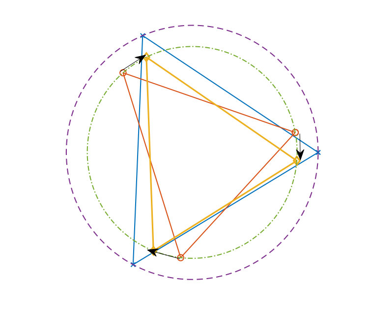 Figure 1
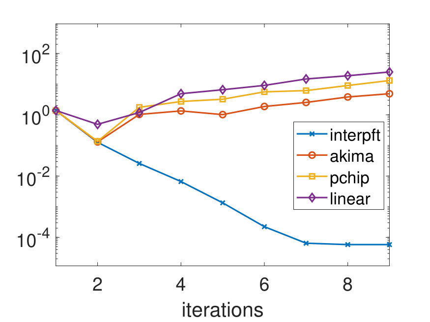 Figure 2
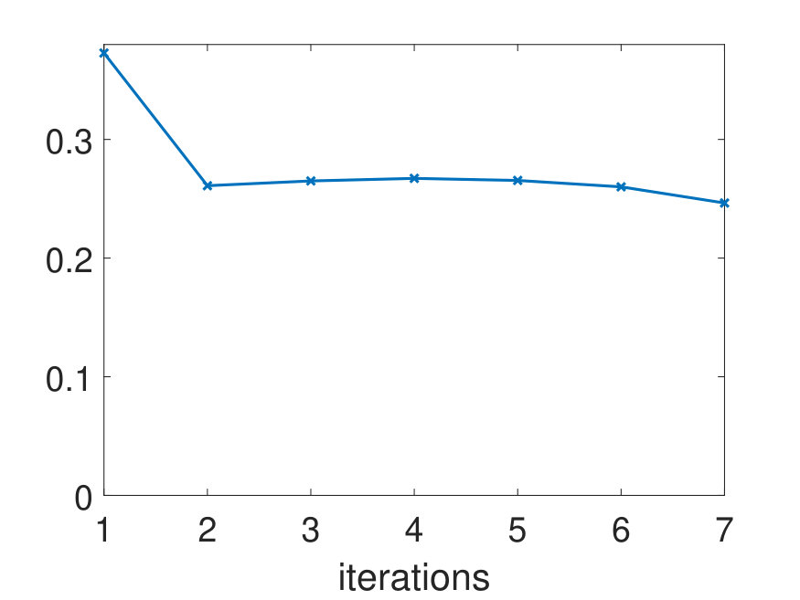 Figure 3
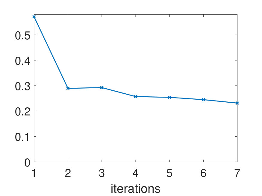 Figure 4
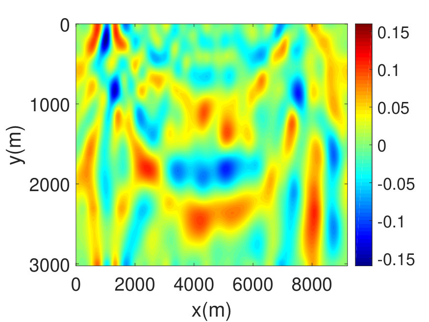 Figure 5
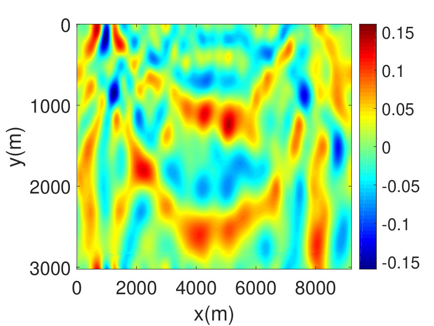 Figure 6
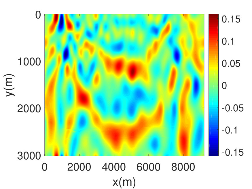 Figure 7
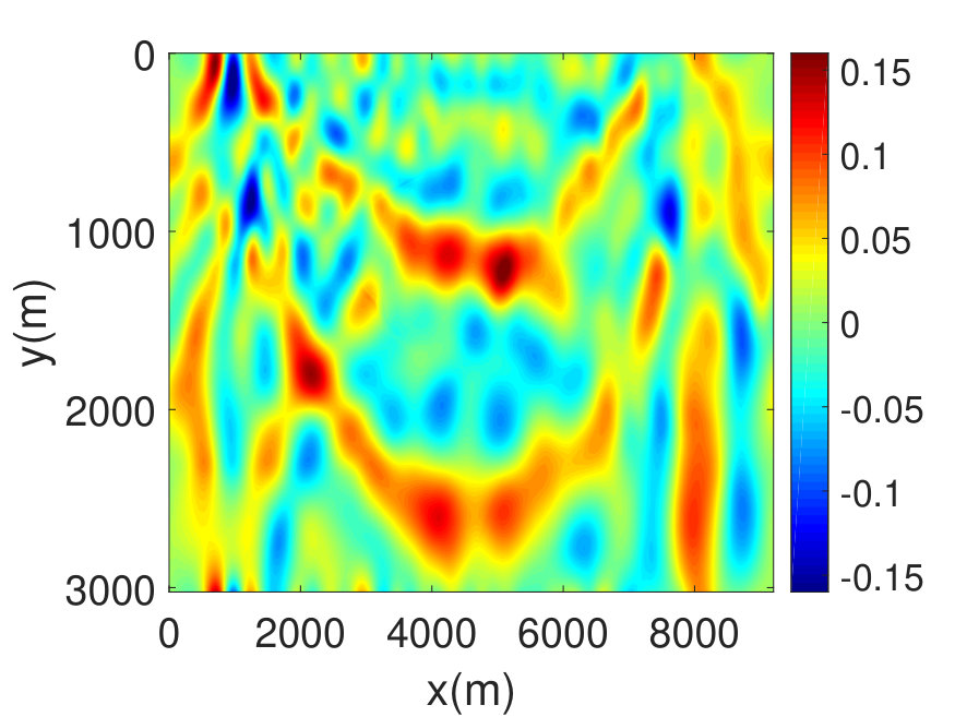 Figure 8
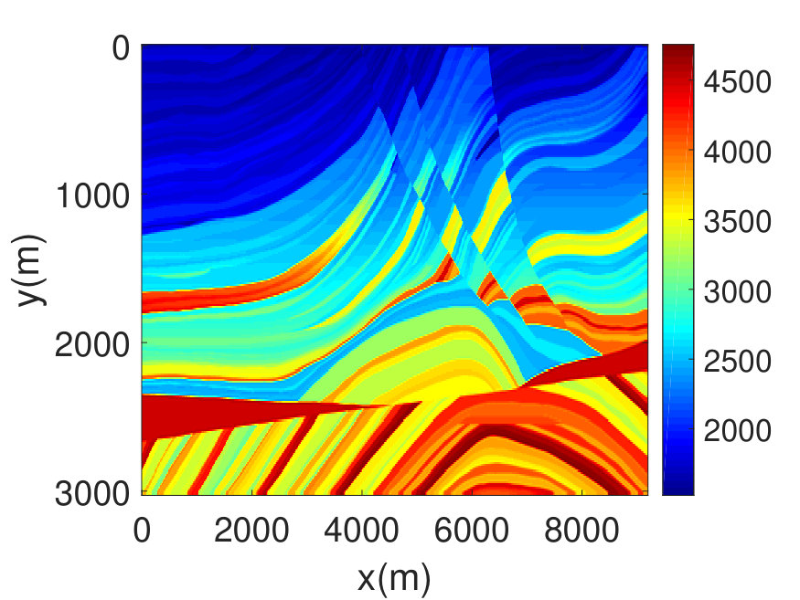 Figure 9
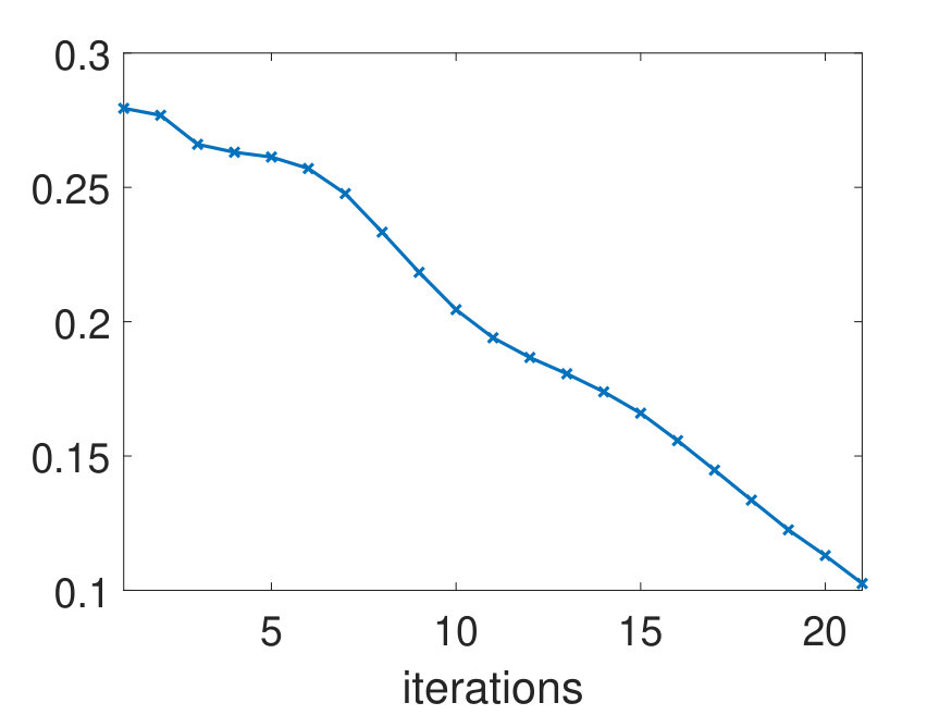 Figure 10
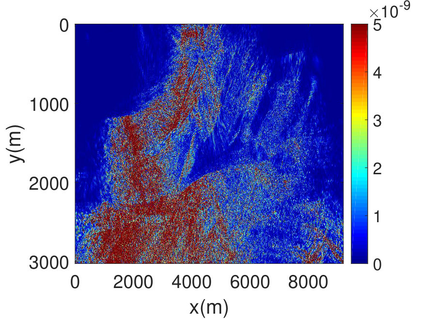 Figure 11
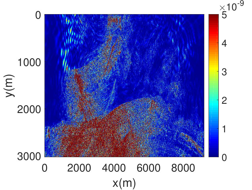 Figure 12
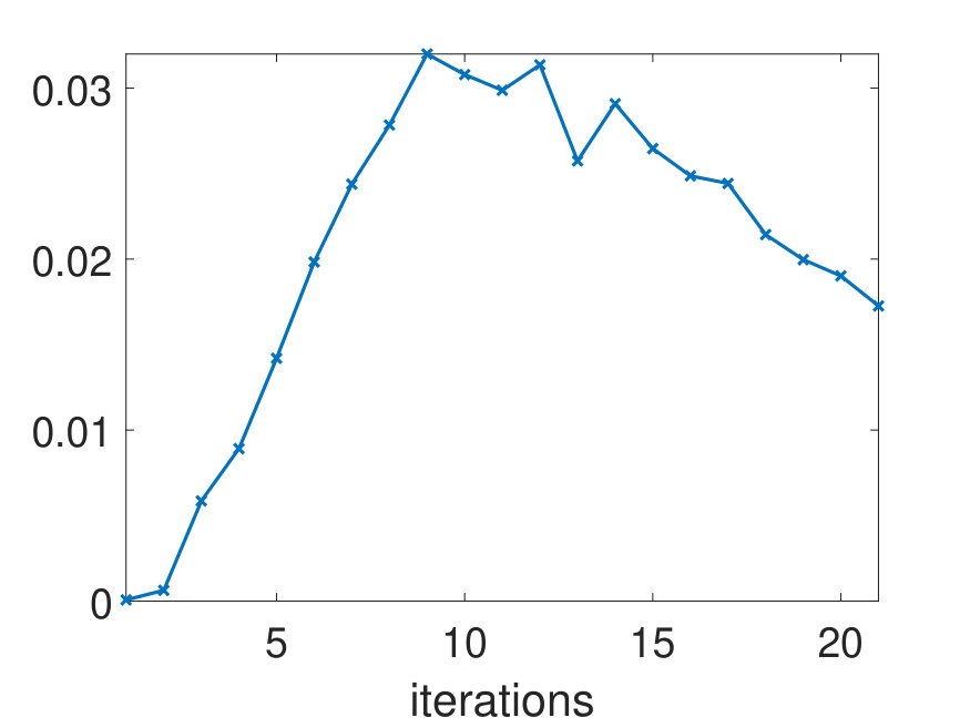 Figure 13
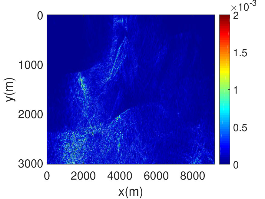 Figure 14
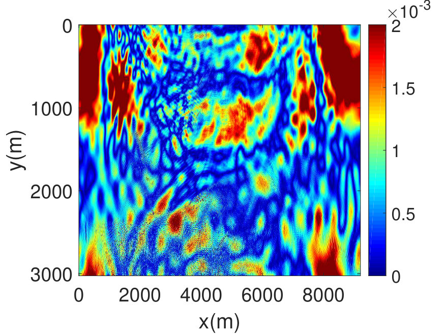 Figure 15
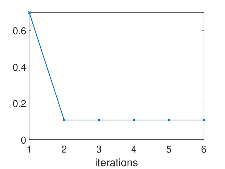 Figure 16
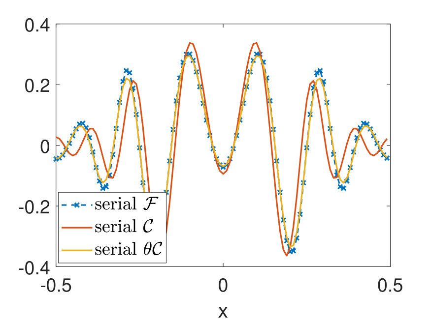 Figure 17
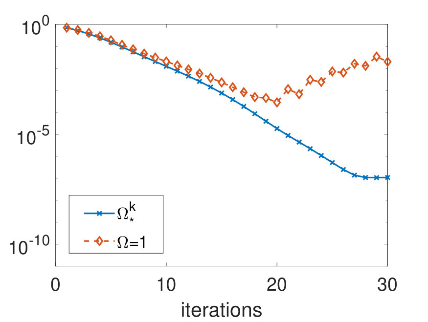 Figure 18
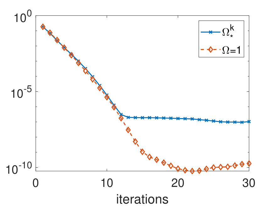 Figure 19
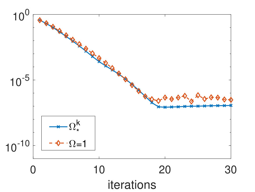 Figure 20
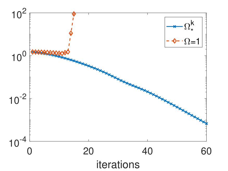 Figure 21
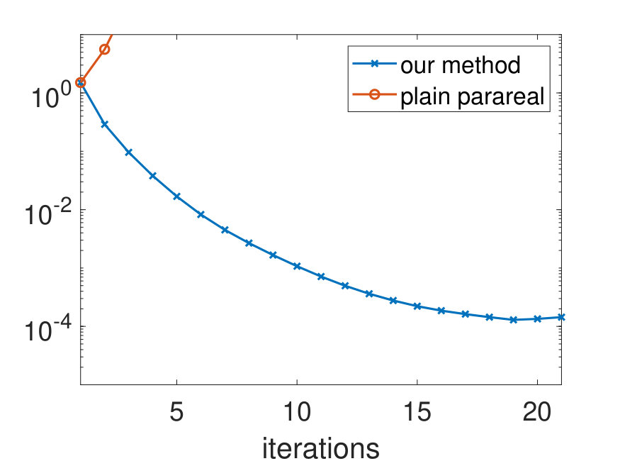 Figure 22
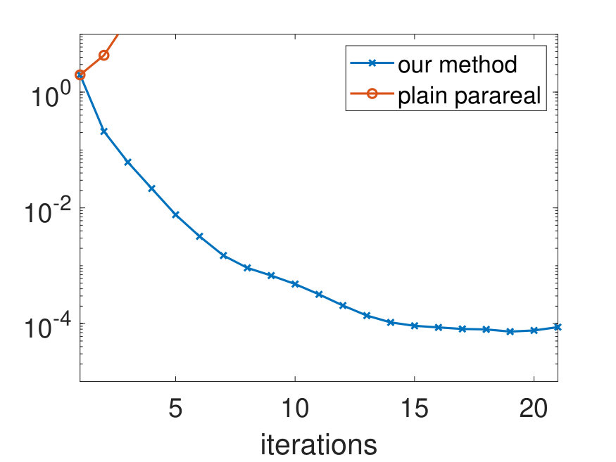 Figure 23
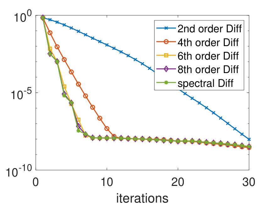 Figure 24
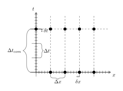 Figure 25
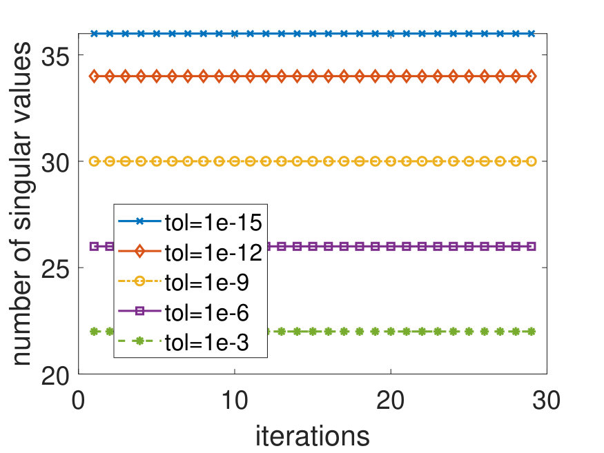 Figure 26
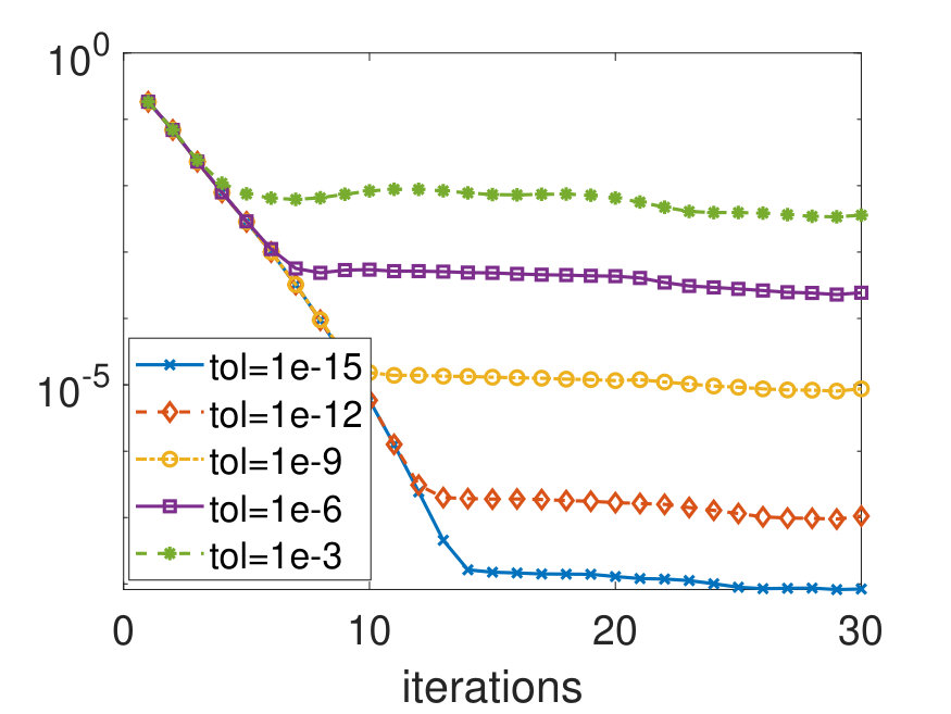 Figure 27
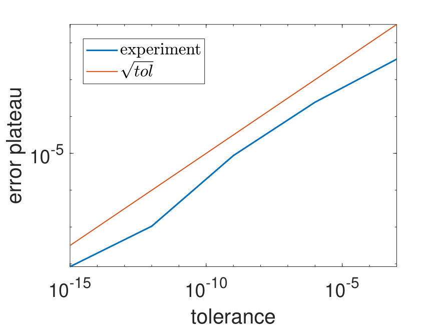 Figure 28
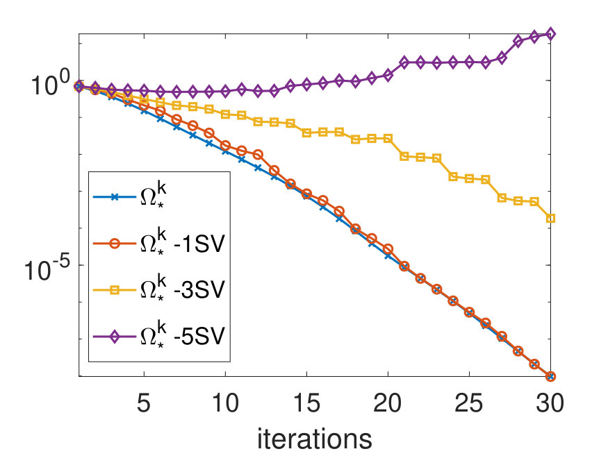 Figure 29
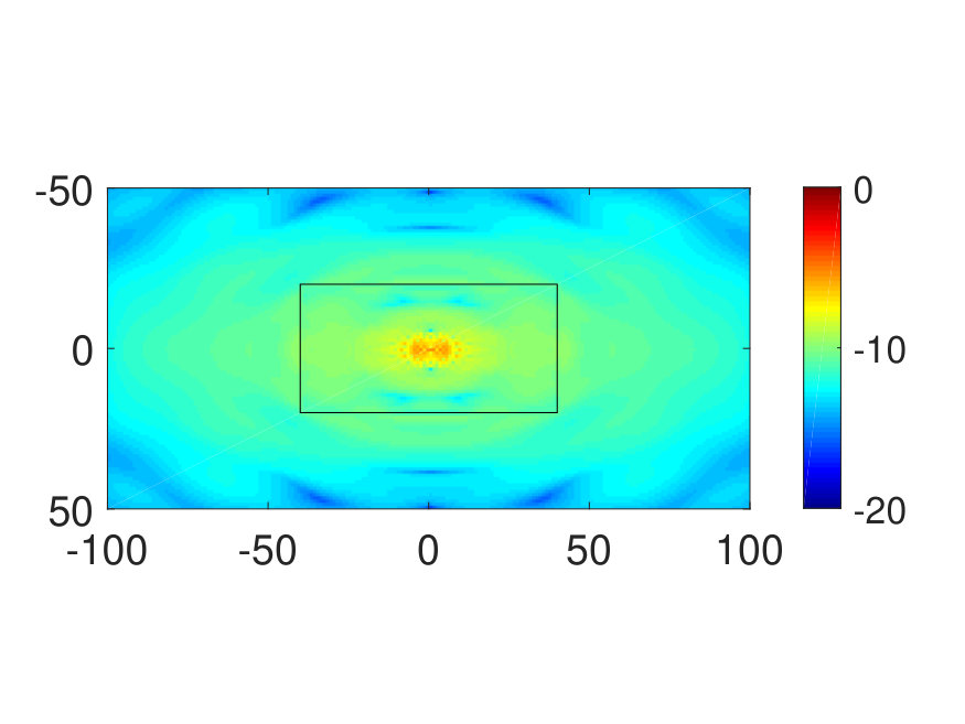 Figure 30
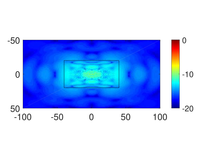 Figure 31
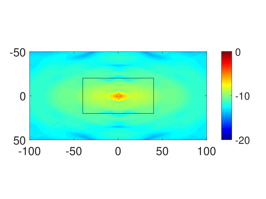 Figure 32
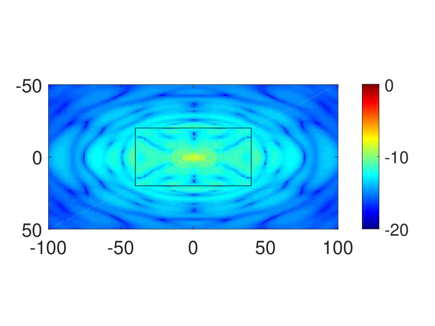 Figure 33
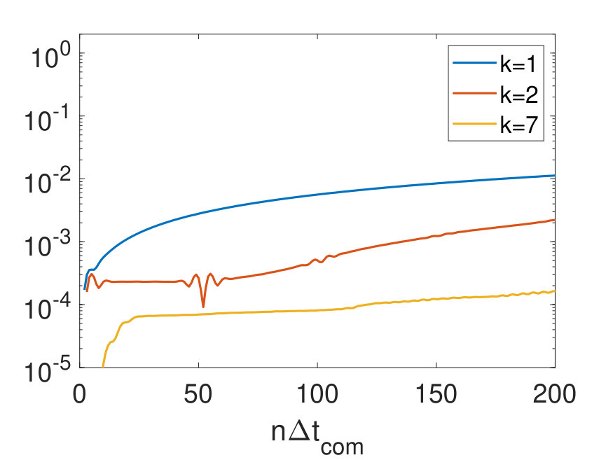 Figure 34
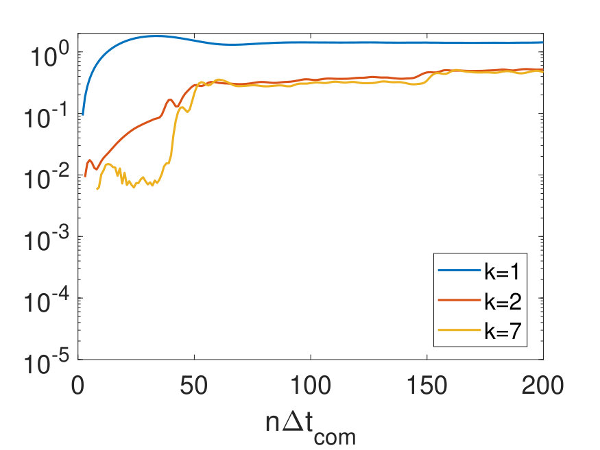 Figure 35
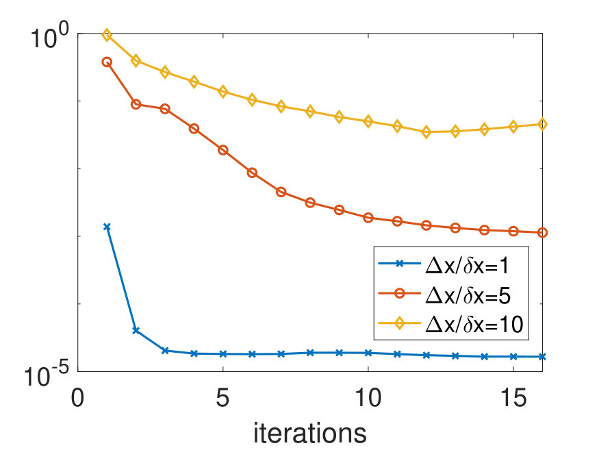 Figure 36
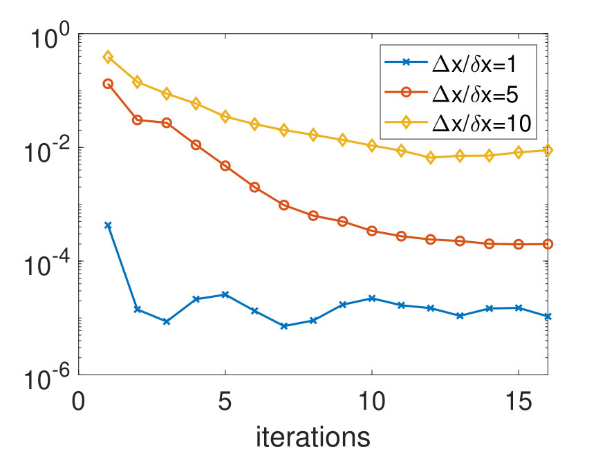 Figure 37
| Cores |
|
Creating corrector |
|
|
|
|||||||||||||
| 20 |
|
0.26 0.11 0.13 0.15 |
|
334.49 |
|
|||||||||||||
| 100 |
|
0.48 0.49 0.64 0.74 |
|
1724.30 |
|
|||||||||||||
| 4 | 200 |
|
0.81 1.06 3.14 1.77 |
|
3479.63 |
|
||||||||||||
| 20 |
|
0.95 0.1 0.11 0.14 |
|
333.78 |
|
|||||||||||||
| 100 |
|
0.46 0.49 0.57 0.73 |
|
1725.16 |
|
|||||||||||||
| 8 | 200 |
|
0.99 1.08 1.39 1.94 |
|
3491.95 |
|
||||||||||||
| 20 |
|
0.26 0.11 0.11 0.13 |
|
332.83 |
|
|||||||||||||
| 100 |
|
0.46 0.46 0.58 0.72 |
|
1734.02 |
|
|||||||||||||
| 20 | 200 |
|
1.06 1.03 1.35 1.73 |
|
3492.86 |
|
Peer Reviews
No public reviews on file for this paper yet. If you reviewed it on a platform where reviews are public (OpenReview, ICLR, NeurIPS, ICML), you can paste yours below so the community can read it here.
Videos
No videos yet. Explain this paper in a talk, walkthrough, or lecture? Add one.
A stable parareal-like method for the second order wave equation
Hieu Nguyen
and
Richard Tsai
Abstract.
A new parallel-in-time iterative method is proposed for solving the homogeneous second-order wave equation. The new method involves a coarse scale propagator, allowing for larger time steps, and a fine scale propagator which fully resolves the medium using finer spatial grid and uses shorter time steps. The fine scale propagator is run in parallel for short time intervals. The two propagators are coupled in an iterative way that resembles the standard parareal method [24]. We present a data-driven strategy in which the computed data gathered from each iteration are re-used to stabilize the coupling by minimizing the wave energy residual of the fine and coarse propagated solutions. Several examples, including a wave speed with discontinuities, are provided to demonstrate the effectiveness of the proposed method.
Key words and phrases:
Keywords: parallel-in-time, wave equation, Procrustes problem
Oden Institute for Computational Engineering and Sciences, The University of Texas at Austin, TX 78712, USA. E-mail: [email protected]
Department of Mathematics and Oden Institute for Computational Engineering and Sciences, The University of Texas at Austin, TX 78712, USA and KTH Royal Institute of Technology, Sweden. E-mail: [email protected]
1. Introduction
In this paper, we will focus on the initial value problem of the standard second order wave equation:
[TABLE]
For boundary conditions, we consider either periodic, absorbing boundary conditions or placing a perfectly matched layer around . The wave speed is given explicitly and independent of the solution. Our objective is to develop a stable parallel-in-time algorithm for (1).
The wave equation is a physical model for seismic wave and electromagnetic wave in certain simplified setups. It is also used as a test case for developing algorithms that are further generalized to more complicated elastic and electromagnetic wave equations.
Time domain decomposition methods for evolution problems has been of increasing interest in the partial differential equation community due to the increasing number of cores available in modern supercomputers. Despite rapid advance in parallel computer architecture, parallelizing the time evolution of the second order wave equation efficiently is still a challenging problem. One of the time domain decomposition paradigms is parallel-in-time method. The whole time domain is partitioned into subintervals for parallel processing. The most relevant algorithm to this paper is the parareal method introduced by Lions, Maday and Turinici [24]. The parareal method combines iteratively two propagators, denoted by the fine propagator and by the coarse propagator. They approximate the solution propagated from . The approximate solution at parareal iteration , denoted as , can be described by
[TABLE]
Note that for each , is computed in parallel. For the second order wave equation under consideration, is a vector corresponding to .
Typically, the coarse propagator runs on coarse grid and is cheaper to compute, while the fine propagator runs on finer grid and is assumed to fully resolve the small scales in the problem. The finer propagator is thus more costly to compute.
In [4], it is shown that the parareal method is stable and converges linearly to the serial fine solution if the coarse propagator is smooth and has sufficient dissipation. When certain conditions are met, the parareal method can achieve high fidelity solution within few iterations. Some applications of the parareal method are: plasma turbulence in Tokamak reactor [38, 37, 36], Navier-Stoke equations [14, 40, 11], acoustic wave [28], shallow water [20], chemical kinetic [6], molecular dynamics [9], reaction wave [13], neutron diffusion [5, 26], lattice Boltzmann equation for laminar flow [29, 23, 30].
Speed up of wall-clock time is attained when the coarse propagator can be chosen as a spatial coarsening of the fine propagator [35, 33] which allows larger coarse time step. Indeed, this coarsening technique provides additional speed up in some applications [25, 3, 23] because the coarse propagator has less grid points to compute, provided an appropriate grid restriction and interpolation operator. However as shown in [33], considerable coarse grid resolution and accurate interpolation are required in order to make the parareal iteration (2) converge.
The parareal method tends to suffer from slow convergence or instability when applied to hyperbolic problems. Using an oscillatory dynamical system as an example, [1, 2, 22] pointed out that the phase error between the coarse and fine propagators is the reason for the slow convergence. Analogously for advection problems, the authors in [34] observed that numerical dispersion between the solvers makes the parareal method converge from above and hence causes instability. Intuitively, constructive or destructive interference of two overlapping plane waves depends on their relative phase which is sensitive to the frequency, yet the parareal iterative coupling (2) is point-wise in space and time.
There have been some attempts to modify the classical parareal method in order to address the slow convergence issue. In [12], the fact that solutions to the wave equation live on a submanifold of constant energy is exploited. In that work, the solutions are projected onto the submanifold to stabilize the parareal iterations. More precisely the algorithm can be presented as
[TABLE]
where denotes the projection onto the constant energy submanifold. However, the projection is obtained by solving nonlinear equations which can be sensitive to the initial guess.
In the so-called Krylov-subspace enhanced parareal methods [15, 35], computed solution data is used to construct projection operators, which is used to modify the coarse propagator. To get the projection operator , a set of orthogonal vectors is constructed for the subspace spanned by for . Let be the matrix whose columns are the orthogonal vectors , then . The enhanced parareal algorithm takes the following form:
[TABLE]
where is the identity. The enhanced coarse propagator corresponds to
[TABLE]
The fine propagation, for is the orthogonal vector that defines , is precomputed and stored. The precomputation incurs an additional computing cost on top of orthogonalization of the data matrices.
The reduced basis parareal method [10] develops more efficient ways to construct the basis vectors and extends the approach to solve nonlinear equations.
The convergence and stability of these methods are analyzed and demonstrated by numerical examples of constant wave speed media in one and two dimension. However, in these work, the fine and coarse solvers are assumed to work on the same spatial grids and examples of variable wave speed are not presented. In this paper, we will consider the solvers on different spatial grids and present examples with variable wave speed. We also use the computed data, but its usage is very different from [15, 35, 10], see Section 3.2.
On the other hand, it is known that the slow convergence and instability of the parareal method for hyperbolic problems can be due to some notions of phase errors [2, 1] and numerical dispersion [34]. In [1], effective multiscale parareal schemes relying on elaborate phase correction are proposed for a class of highly oscillatory dynamical systems. In [2], we derived convergence theory for a modified parareal scheme applying to linear systems of ordinary differential equations (ODEs). Additionally, in that work, we investigated a few simple strategies of phase correction systematically and showed that appropriate phase correction could enable the resulting scheme to have superior performance.
In this paper, we propose a new method, based on the idea of -parareal scheme [2]. Instead of decomposing the input data as in [15, 35], we use the computed data to build an operator, formally denoted as , that directly brings the coarse solutions, , closer to the fine solutions, . In this paper, the operators are constructed by minimizing the residual between the fine and coarse solutions in a semi-norm related to the discrete wave energy.
2. Preliminary background
We briefly review the plain parareal method and its properties. In a context of linear evolutionary problem for and linear function, let us denote the fine propagator/solver and the coarse propagator/solver . Then the plain parareal iteration can be written as a recurrence relation
[TABLE]
Starting solution is the serial coarse solution . In addition, by rewriting the recurrence relation (3) in a matrix form and manipulating the inverse of Toeplitz structure, an error estimate is derived in [2]
[TABLE]
The first term on the right hand side is equivalent to the local truncation error of the coarse propagator, assuming the fine solver is an exact one. The summation term is bounded above by for stable schemes, e.g. . Above error estimate is equivalent to linear convergence analysis of the parareal method derived in [4, 16].
Wall-clock complexity of the parareal algorithm is estimated by
[TABLE]
Comparing to the complexity of the serial fine solver , the parareal algorithm is more effective (from the perspective of total wall-clock computing time) if (i) a large number of computing cores, , are used; (ii) the coarse/fine time stepping ratio is sufficiently large ; and (iii) the number of iterations, needed to for the desired accuracy , is small.
The key objective of this paper is to introduce a data-driven strategy to stabilize and improve the efficiency of the parareal iteration.
3. The proposed method
We propose a scheme that takes the general form:
[TABLE]
Here, denotes the solutions computed on the grid, and it has two component blocks, one corresponds to the wave solution and the other the time derivative . In this paper, for readability we shall also use to denote the time derivative of , i.e. . The coarse and fine propagators, and will operate on different grids, and additional interpolation and restriction operators are needed for coupling the two propagators. Here we use and to denote the appropriately defined operations to be described in detail in this section.
A family of operators are constructed such that
[TABLE]
Clearly, direct calculation of is not practical because it undermines time parallelization of the -parareal method. Instead, we seek an effective mapping that has similar property as and is constructed from data computed along the parareal iterations.
3.1. Discretizations and data preparation
In this paper, we use the uniform Cartesian grids for the spatial domain and uniform stepping in time. Both the coarse and the fine propagators are defined by the standard second order central difference scheme for the spatial derivatives and velocity Verlet for time marching. The coarse propagator will operate on the coarse grid: and the fine propagator will operate on the fine grid: for or .
Let denote respectively the solutions computed at time on the fine and coarse grids. are the number of grid points for the fine grids and the coarse grids respectively.
These fine grid functions and coarse grid functions are coupled by an interpolation and a restriction . The accuracy of the interpolation method will influence the stability of parareal iteration, as discussed in Section 6.4. Coarse propagator uses point-wise value of the wave speed and does not involve averaging of the wave speed nor homogenization of the wave equation. The fine and coarse propagators communicate at The fine propagator uses the step size and the coarse propagator uses , with selected according to and for stability in the respective time stepping. See Figure 1.
Given at , the fine and coarse propagators are applied to obtain the solutions to define
[TABLE]
and
[TABLE]
For readability, we will write in-line vector and full vector
[TABLE]
interchangeably. These solutions are propagated over a coupling time interval . These propagators are expected to approximately preserve the wave energy.
Finally, we will quickly describe the data matrices that will be used to construct the operators . We are interested in using the computed solution data, particularly the gradient of the wavefield and a weighted momentum of . Each column of data matrices is formed by block(s) of the gradients followed by a block of momentum of coarse grid solution at -th coupling time. In practice, the gradient operator, , will be replaced by some numerical approximation . Then define the data:
[TABLE]
[TABLE]
Here and for the rest of the paper, denotes the component-by-component multiplications of and . The same convention is used for
Now, define the discrete wave energy function as
[TABLE]
We see that it is equivalent, up to a constant, to the Frobenius norm of the :
[TABLE]
3.2. Minimization of coarse-fine solution gaps
For simple plane waves, it is well known that the phase error, not the amplitude difference, between coarse and fine solutions, causes the parareal iteration to converge slowly or diverge [35, 22]. If two plane waves are in phase, parareal style updates can effectively correct the amplitude error. For general wave solutions, it is inconvenient to work with the phase notion defined by the plane wave solutions. Instead, we consider the discrete wave energy semi-norm (9) which is induced by the inner-product of the energy component vectors, i.e. the columns of in (7) and (8). Such inner-product gives us a notion of angle between two wave solutions. The proposed strategy to stabilize the parareal iteration is by minimizing the inner-product between coarse and fine energy component vectors without changing their norm. Similar strategies of using wave energy to compare wavefields for wave propagation purposes have been used successfully, for example in seismic imaging [31], wavefield approximation by Gaussian beams [39].
Denote the -th column of and by and respectively. We consider the following optimization problem:
[TABLE]
Recall that the elements in the columns of and consist of the spatial gradients and weighted time derivatives of the solutions on the respective fine and coarse grid, and that the norm corresponds to the discrete wave energy (9). Therefore, we look for a unitary matrix so that the discrete wave energy of the corrected coarse solutions is the same as before correction. Intuitively the correction operator aligns the phase (in the above sense) of the coarse solution to fine solution for each . It is similar to the local phase-alignment procedure in [1] as depicted in Figure 2. Indeed, from each term in the summation
[TABLE]
the minimization can be interpreted as minimizing the sum of the angles between the columns on the data matrices. Thus, we shall refer to as the phase corrector.
The minimization problem (11) is equivalent to the ”Procrustes Problem” [17]:
[TABLE]
where denotes the Frobenius norm of a matrix. An in-depth review of the Procrustes problem can be found in [18]. Its variants have been instrumental to multidimensional statistical analysis, rigid body motion simulation, satellite tracking and machine learning [42, 32, 19].
3.3. Solution to the optimization problem
The optimization problem (11) can be solved in a couple of different ways. One of them is to use the singular value decomposition (SVD) of the correlation matrix
[TABLE]
If matrix has full rank, the minimizer of (11) is uniquely
[TABLE]
where are the left and right singular vectors of . Correspondingly, the minimum residual is
[TABLE]
Figure 2 illustrates the Procrustes problem and its solution in a simple setup in .
3.3.1. Low rank approximation of
We now consider a low rank approximation of for computational efficiency. Since the number of time slices is usually much smaller than the number of (coarse) spatial grid nodes, i.e. , we can factorize the data matrices using the reduced QR factorization. Denote the factorizations by and , where
[TABLE]
With the singular value decomposition of the smaller system , the correlation matrix can be factored into
[TABLE]
The last relation shows that
[TABLE]
Hence we can use the factorization of the smaller matrix to obtain
[TABLE]
By setting a tolerance to singular values in , there are singular values such that remained. As the result, we only need to store number of columns in , and the truncated phase corrector becomes
[TABLE]
3.3.2. Enriching the phase corrector
After every parareal iteration, more data becomes available. We can use this data to enrich the phase corrector. Define
[TABLE]
The singular value decomposition of can be updated using that of , see [7]. We summarize the update procedure is Algorithm 1.
3.4. Reconstruction of wavefield from the gradient
After correcting the energy components, i.e. the gradients and the weighted time derivatives, of the coarse solutions, it is necessary to reconstruct the wavefield pair from the corrected energy components. In other words, we denote as the corrected energy components of a wavefield pair
[TABLE]
where the mapping takes function to wave energy components. Then we want to deduce the corrected wavefield pair such that
[TABLE]
It is straightforward to find the latter component . For the displacement component , we use the spectral property of differentiation to recover its the Fourier modes as follow
[TABLE]
We denote this mapping from energy component to wavefield component as . In particular, when the gradient is approximated by Fourier method, this reconstruction is an identity.
Proposition 3.1**.**
Suppose the gradient of function is estimated by spectral method , then
[TABLE]
Proof.
Let
[TABLE]
Since maps function to energy components we have
[TABLE]
By construction of , for nonzero wavenumber
[TABLE]
Here the gradient is approximated using spectral method then
[TABLE]
And for zero wavenumber , Thus, while the second energy component This concludes that the mapping is equal to identity. ∎
If the gradient is approximated by a central finite difference of -order instead of the spectral method, for one dimensional setting equation (20) in the proof above becomes
[TABLE]
where are appropriate coefficients of the difference stencil. When the spatial grid is small enough above expression is approximately
[TABLE]
Particularly for the second order central difference , we would have , then
[TABLE]
which says that because .
In practice, we observe that the algorithm does not require spectral approximation of the gradient, but instead is necessary for stability of the method. When central finite difference is utilized, it is well known that the modified wavenumber is less than , hence central difference satisfies the requirement . Algorithm 2 summarizes above procedure.
3.5. The proposed algorithm
The proposed algorithm couples the fine and the coarse propagators at times over the fine grid (the spatial grid that the fine solutions are defined). However, it is important to note that the phase corrections are applied on the coarse grid. If the two grids are not identical, an interpolation is needed. We denote the interpolation operator by . Furthermore, denote the mappings between the wavefield and its energy components by and . With these notations, the operator after iterations can be written as
[TABLE]
Here we use to denote the phase corrector derived from the data matrix .
Finally, our new algorithm can be written compactly as in -parareal form
[TABLE]
Algorithm 3 describes the new scheme in a pseudo-code form with more details.
Similar to the Krylov subspace method [15, 10], our method requires orthogonalization of data matrices, but they are formed in a different way. In this paper, the data matrices are the multiplication of the wave energy components of the fine data and the coarse data as in equation (14). Then the phase correctors are constructed from the singular value decomposition of the data matrices. In [15, 10], the data matrices, consisting of computed solutions, are orthogonalized to form projection operators. In contrast, our phase correctors are not projections, but they effectively induce translation of the coarse solutions on constant energy submanifolds.
4. Complexity Analysis
There are three parts to our implementation: parallel fine propagator computation, construction of and the serial coarse updates. We assume that (i) no spatial domain decomposition, i.e. whole domain on a single core, (ii) standard QR complexity, i.e. no multithreading, (iii) communication between nodes and other tasks negligible.
In each iteration, the wall clock complexity for the parallel fine and coarse computations is in the order of
[TABLE]
where is the number of cores, are respectively the total number of fine and coarse grid points. The complexity of serial coarse update in an iteration is
[TABLE]
The complexity of standard QR factorization for constructing is
[TABLE]
Therefore, the total complexity is
[TABLE]
where is the number of iterations. In this set up, the speed up over a serial fine computation is
[TABLE]
Additionally, we have coarse/fine time step ratio , which implies , and their corresponding the mesh ratio is . Hence the theoretical speed up is
[TABLE]
We note that the third term in above speed up is derived from the classical complexity for QR factorization (of matrices of fixed number of rows). The speed up analysis (32) presents the worst-case asymptotics as N approaches infinity. In practice, we observe that QR factorization has sub-quadratic scaling when multithreading, ubiquitous in modern computers, is enabled. However, to our knowledge, speed up analysis of QR in a multithreading environment is not straightforward. To illustrate the effectiveness of multithreading in computing QR factorization, consider random matrices with fixed number of rows and vary the number of columns in a way relevant to the paper. The computing time is presented in Figure 3. The computing time roughly grows as the power of of the number of columns, rather than quadratically according to the classical QR complexity. We also see that having 68 threads speed up the computation by more than a factor of 10. Finally from numerical experiments, the QR step in our algorithm takes relatively small amount of time compared to other components, see Section 7.2.4.
5. Stability and convergence
In this section, we will derive some estimates that show the stability and the convergence of algorithm 3 under certain assumptions. We measure the difference, in the discrete energy semi-norm on the coarse grid, between the serially computed fine solution and the iterated solution.
Consider energy components of parareal iterated solution restricted on the coarse grid
[TABLE]
Its parareal iterative coupling is expressed as equation (29)
[TABLE]
Recall that , so
[TABLE]
Since the restriction operator takes point wise values, it cancels action of the interpolation . So equation (33) becomes
[TABLE]
Let us denote the square root of wave energy as , where is defined in (9). Thus,
[TABLE]
Theorem 5.1**.**
Suppose that
- (1)
the coarse propagator satisfies, for some ;
[TABLE] 2. (2)
the residual of the energy minimization problem is bounded uniformly for :
[TABLE]
where are data matrices in (7),(8) gathered in the first iterations; 3. (3)
, and \|1-\Lambda^{\dagger}\Lambda\|_{2}<\lambda{\color[rgb]{0,0,0}\definecolor[named]{pgfstrokecolor}{rgb}{0,0,0}\pgfsys@color@gray@stroke{0}\pgfsys@color@gray@fill{0}\ll}1/N.
Then
[TABLE]
where is a norm equivalence constant between norm (sum of norm of columns) and Frobenius norm.
Proof.
Consider the square root of wave energy of (34)
[TABLE]
We apply triangle inequality to obtain
[TABLE]
By construction, , and by the hypotheses that and energy bound of the coarse propagator,
[TABLE]
we have
[TABLE]
Seeing the third term as part of the energy minimization problem in (10),
[TABLE]
As the above relation also holds for , therefore,
[TABLE]
Applying the discrete Grönwall inequality [21] on index we get
[TABLE]
By the assumption ,
[TABLE]
∎
Next, we will show that, under some hypotheses, the proposed method converges to the solutions computed by applying the fine propagator serially. The hypotheses involve Lipschitz smoothness of the phase corrector, which implies the minimization problem (11) is solved with sufficient accuracy. We shall use the following notation for those reference solutions:
[TABLE]
We measure the overall error on the fine grid as the square root of the difference in the discrete wave energy:
[TABLE]
Hypothesis 5.1**.**
(i) The phase corrected coarse solution is Lipschitz continuous in energy
[TABLE]
Let denote the overall perturbation
[TABLE]
(ii) The energy error between fine and corrected coarse operators is Lipschitz continuous
[TABLE]
Theorem 5.2**.**
Suppose that the fine and corrected coarse operators satisfy Hypothesis (44) and (51). Then,
[TABLE]
Proof.
In the following expansion of the parareal iteration, the superscript in are dropped for brevity
[TABLE]
It can be verified that the serial fine solution also satisfies above expression when superscript are dropped in solution vector . Then we have an expression for the difference of the solutions
[TABLE]
Recall the square root of energy error is defined as
[TABLE]
Using triangle inequality on with equation (57) we obtain
[TABLE]
Apply equation (44) in Hypothesis 5.1 (i) to bound each term
[TABLE]
Finally we use equation (51) in Hypothesis 5.1 (ii) to obtain
[TABLE]
Thus
[TABLE]
By assumption and , the error goes to zero as approaches infinity. ∎
We see that the convergence depends on the Lipschitz constant in Hypothesis 5.1 (ii), which reflects the gap between the corrected coarse propagator to the fine propagator. This gap between propagators is quantified by the energy residual of the minimization (13).
6. Numerical Study of the New Algorithm
In this section, we study the influence of different components of the proposed algorithm to the overall stability and accuracy. From Section 6.1 to Section 6.4, we consider the influence of (i) varying the low-rank approximation of the optimal phase correctors , (ii) effect of the phase corrector and the parareal update, (iii) different orders of approximation for the gradient and interpolation operator Regarding to the last item, we will use the following interpolation methods, written as MATLAB functions, in this section:
- •
interpft: Fourier interpolation
- •
akima: cubic Hermite interpolation
- •
pchip: cubic interpolation
- •
linear: linear interpolation
From Section 6.1 to Section 6.4, we shall consider the simplest one dimensional setting with for both coarse and fine propagator, and the initial data:
[TABLE]
For Section 6.5, we consider random subsampling of the data matrices to exploit their observed low rank property. In this study, we consider a two dimensional problem with variable wave speed.
We will assume that the coarse grid nodes overlap with the fine grid nodes, and that the restriction operator is just a point-wise evaluation on the coarse grid nodes.
The errors at final time are defined as square root of energy of difference on the fine grid
[TABLE]
And similarly the error can also be defined in of difference in displacement component
[TABLE]
The reference solution are serially computed using the fine propagators.
6.1. Rank tolerance of the phase corrector
In this example, we study the sensitivity of the algorithm to rank-truncation of the optimal phase corrector We use the same spatial grid for both the coarse and the fine propagators in order to avoid error coming from interpolation/restriction. The fine propagator has an CFL number that is 20 times smaller than the coarse, and the coupling take place every 10 coarse steps. We sample several values for tolerance in Algorithm 1 at . The parameters are tabulated below:
[TABLE]
Figure 4 shows the relative energy error along with the iterations as the tolerance in the truncation of is varied. The errors decrease in the first few. The rate of decrease seem independent of the chosen tolerance values. As more iterations progress, the errors convergence eventually stagnate at certain values that strongly correlate to the chosen tolerance values. Particularly, the stagnated error values scale as the square root of the tolerance as shown on the right plot of Figure 4. This scaling can be explained by the fact that the tolerance corresponds to the truncation of , which modifies the wave energy components, and we measure the square root of wave energy difference. Hence in general, the convergence rate of our method is expected to slow down after the error has passed because the tolerance can only be as small as machine epsilon . Figure 5 shows the number of retained singular values for different values of tolerance.
6.2. The effect of phase correction ()
Assuming again that the coarse and fine propagators are on the same grid. Without the phase correction, i.e. , the proposed iteration takes the form
[TABLE]
The above expression becomes the plain parareal method if the term . But when the first wave component is approximated by some finite difference, the term in general. In particular when is approximated by the standard second order central difference, i.e. , corresponds to multiplication of
[TABLE]
to the Fourier mode of the solutions. Since , damps high frequency modes, and thus stabilizes parareal-like iterations.
Nevertheless, for long time simulations, such high frequency damping may be insufficient to stabilize the parareal-like iterations. To illustrate this, we take the same discretization as above but now consider four terminal times :
[TABLE]
*:{\color[rgb]{0,0,1}\definecolor[named]{pgfstrokecolor}{rgb}{0,0,1}\{2.5,5,10,50\}}. Figure 6 presents a comparison of the errors computed with and with , for different terminal times. For shorter time intervals, such as , the two choices of yield similar convergence rates until after some iterations when the errors computed with plateau around a much larger value. For larger terminal times, , the instability that comes with using becomes more and more apparent, while the computations with remain stable.
6.3. The effect of parareal-like corrections
If the parareal-style additive correction is omitted, solution is propagated with just the phase corrected coarse propagator:
[TABLE]
The simulation parameters are given as follow
[TABLE]
We first point out that if preserves the discrete wave energy, then the above scheme will also preserve it by construction of . Figure 7 shows the errors comparing to the serial fine solution. At iteration , the solution is serially computed with the coarse propagator . At iteration , a phase corrector is constructed based on the data computed in . The solution at is serially computed with . On the right subplot of Figure 7, we see that the coarse solution now has the same phase as the fine solution, but has a slightly different amplitude. For iteration after , however, the error does not decrease further since the parareal-style additive correction has been omitted. Comparing to the examples with similar simulation parameters presented in the previous subsection, we see that the parareal-style correction
[TABLE]
is important, as it adds the missing amplitudes back to improve accuracy (when the solutions are properly aligned).
6.4. Influence of interpolation and gradient approximation
So far in this section, we have only considered examples in which the coarse and fine propagators operate on the same spatial grid. When these propagators are on two different grids, interpolation is needed to couple the solutions. In this subsection, we study the effect of interpolation. To illustrate this point, take coarse/fine grid ratio to be 2 and keep the discretization as before
[TABLE]
*:{\color[rgb]{0,0,1}\definecolor[named]{pgfstrokecolor}{rgb}{0,0,1}\{\texttt{interpfft},\texttt{akima},\texttt{pchip},\texttt{linear}\}}. Input wave speed for coarse propagator is as well. Figure 8 shows the error convergence with different methods for grid interpolation. We observe particularly for this example that the spectral interpolation interpft performs better than the lower order methods because it resolves the initial wave form much better.
We also study the influence of the accuracy in approximating the gradient of the wavefield in forming the data matrices. We observe from the following examples that higher order approximations of gradient estimation accelerates convergence rate of the proposed method. The parameters used in the simulations are tabulated below:
[TABLE]
*:{\color[rgb]{0,0,1}\definecolor[named]{pgfstrokecolor}{rgb}{0,0,1}\{2,4,6,8,spectral\}}. To isolate other factors that can also influence the convergence rate, the table below shows the relative residual in Sec 3.3 averaged over all iterations, denoted as \Bigg{\langle}\|\mathsf{F}-\mathsf{\Omega}^{k}_{*}\mathsf{G}\|_{F}\Big{/}\|\mathsf{F}\|_{F}\Bigg{\rangle}_{k}. We see that the residual does not change while we increase the order of finite difference. In the last column, the errors in reconstruction of from the its approximated gradient is provided. To be specific, we denote operation in equation (18) as .
[TABLE]
Figure 9 shows the convergence of errors for different central differencing and Fourier approximations for . The ones with second order approximation has the slowest convergence rate, while those using sixth order or higher converge faster.
6.5. Random subsample of the data matrices
We point out here that the cost of the stabilization can be further reduced by certain randomized algorithms [41, 27]. These randomized algorithms exploit the observed low-rank nature of our data matrices. Another approach is directly subsampling the data matrices. To illustrate the low-rank property, consider a plane wave in a 2D wave guide
[TABLE]
with the following discretization
[TABLE]
After each parallel computation of coarse and fine data , we plot the normalized strength of singular values of the correlation matrix for a few iterations in Figure 10.
The normalized strength of the singular values drops exponentially in this particular example. A quick and simple strategy to exploit this low-rank property is to randomly sample time slices in matrices and . By reducing the sample size, the data matrices becomes thinner so that QR factorization is faster. We compared the convergence of different sample sizes in Figure 10.
7. Numerical Examples
In this section, we shall consider one and two dimension examples, including an example that involve a large scale wave speed model commonly used in the seismic migration community. When the spatial grid of coarse and fine are different, wave speed on the coarse grid is point wise evaluation of the given wave speed.
7.1. One dimensional examples
Consider a medium with the wave speed
[TABLE]
and the initial wavefield in
[TABLE]
We present a numerical simulation using the parameters listed below:
[TABLE]
The fine propagator operate on a spatial grid which is 10 times finer than the coarse grid, and uses a CFL which is 10 times smaller. Figure 11 shows convergence of the proposed method comparing to the plain parareal. Because fine and coarse solution in a variable medium may differ a lot, the plain parareal method becomes even more unstable.
7.2. Two dimensional cases
We apply the proposed method to three types of media: one with a smoothly varying wave speed (wave guide), one containing a piece-wise constant wave speed (inclusion), and a more complicated wave speed profile which is often used in exploration seismology as a standard case study (Marmousi).
7.2.1. Waveguide
We consider a wave guide in -plane with the wave speed
[TABLE]
The initial data is a plane wave traveling left to right along the -axis:
[TABLE]
The parameters used in the simulation are set as follow
[TABLE]
Figure 12 shows error of the solution with different coarse fine grid ratio.
7.2.2. Inclusion
In this example, we consider the two dimensional domain in the -plane where a plane wave encounters an inclusion of radius centered at , modeled by the wave speed
[TABLE]
We used the initial data traveling from left to right
[TABLE]
and discretization parameters
[TABLE]
When the coarse grid is the same as fine grid, the iterations converge to the serial fine solution for the whole time interval (shown in left subplot of Figure 13). On the other hand, when coarse/fine grid ratio is , the right subplot of Figure 13 shows that the error escalates quickly at (or ), when the initial plane wave hits the inclusion for the first time, and again at (or ), as some parts of the initial plane wave wraps around the domain the interact with the inclusion again. The error does not decreasing for later iterations.
Figure 14 shows the relative density error in the Fourier modes of the computed solution at different times. For the short time range (before the wave energy is scattered by the inclusion), most of the error concentrates at low frequencies which the coarse grid is able to resolve. Once the wave touches the inclusion at and thereafter , the errors in the higher frequencies becomes significant. These scattered higher frequency wave is not resolved by the coarse grid and cannot be corrected by the proposed method.
7.2.3. Marmousi experiment
We test our method with the Marmousi wave speed model [8], as shown in Figure 15. The fine scale domain has grid points while the coarse scale has grid points or 50 times smaller in each dimension. The initial data is a pulse waveform centered at where denotes the length unit in meter,
[TABLE]
The discretization parameters are in the following table where coarse and fine computation communicate every coarse time steps
[TABLE]
The computation is executed on one node consisting of cores on the Stampede2 system at Texas Advanced Computing Center (TACC). With our non-optimized MATLAB code, it took 26 hours to run 6 parareal iterations and 12 hours to compute the serial fine solution. Hence each iteration takes about 4 hours, almost 3 times faster on the wall clock than the serial fine computation. For more detailed experiment, see Section 7.2.4.
Figure 16 shows the solutions computed by the proposed method. One observes that some finer details are added back to the computed solution along the iterations. However, Figure 17 reveals that the errors decreases rather slowly after the first few iterations. Indeed, the setup in this experiment is a challenging example of strong scattering due to discontinuities in the wave speed (compared to the previous Example).
It is natural to wonder if the proposed method computes solutions that would converge to the serially computed fine solutions, when the coarse and fine propagators run on the same spatial grid. For this purpose, it suffices to consider a smaller version of the Marmousi velocity model, which is defined on grid points. A different set of discretization parameters are described in the following table
[TABLE]
Figure 18 shows the absolute error and energy error fields at iterations and . On the left column, we see that the solution at has larger point-wise absolute error and energy error in regions of high wave speed contrast (e.g. the lower left region in the image domain) than the regions of low wave speed contrast (e.g. upper left region in the image domain). On the right column, however, the solution at has large patches of point-wise absolute error at regions of low wave speed contrast. These errors contribute to the increase of overall error in the initial few iterations shown in the right subplot in Figure 19.
We observe a discrepancy between the two errors curves. The energy error decreases while the error increases, particularly in the regions of low wave speed contrast. This discrepancy in regions of low wave speed contrast is likely due to the construction of the phase corrector. At regions of high contrast, when locally scattered wave emerged, the phase corrector is constructed to decrease the error there but because it is a global operator, it also perturbs solution everywhere else that in effect increases the overall error.
7.2.4. Timing
To see how wall clock computing time changes as the number of cores changes, we use the Marmousi model again and the discretization parameters are as follow
[TABLE]
We used an Intel Skylake node and varied the number of cores to perform the computation. In Table 1, computing time in seconds is recorded for different parts in the algorithm: parallel computation, creation of the phase corrector (requiring QR), serial coarse update. We see the computing time of the stabilization process is small, relative to other parts of the algorithm. As a benchmark, we also timed the serial fine computation. The projected speed up is calculated as if the number of cores is equal to the number of time slices .
8. Summary and conclusion
We present here a new stable parareal-like method for the second order wave equation. The method uses the solutions computed along the iterations to construct linear operators which bridge the energy difference between the coarse and fine propagators. Such operators are referred to as the phase correctors in this paper. We presented an extensive set of numerical studies which aim at revealing the properties of the proposed method. From the experiments, we see that the proposed method works well for constant and smooth wave speeds.
For piece-wise smooth wave speeds, the algorithm is stable, but does not seem to produce numerical solutions that converge to the solutions computed by the fine propagators (as the number of iterations increase), when the fine and coarse propagators run on different spatial resolution. This is expected because the higher Fourier modes of the solutions computed by the fine propagator on a finer spatial grid cannot be resolved by coarser grids. This is true even when the initial wavefield is resolved by the coarse grid. As our simulations reveal, the stagnation of the errors may be caused additionally by a couple of different approximations used in the algorithm. This paper outline these factors for future improvement. In the last two examples involving piece-wise smooth wave speeds with high contrast, we observe that the relative errors are in general much larger than the previous cases. Most likely, this is due to strong local scattering of waves cause by the discontinuities in the wave speeds. Such scatterings cannot be corrected efficiently by the proposed Procrustean approach.
Finally, if domain decomposition in space is applied, due to the finite speed of propagation nature of wave, we expect that different phase correctors in the subdomains can be constructed in the same way and the resulting algorithm would be stable. This important topic should be investigated more carefully in a separate paper.
Acknowledgment
The authors are supported partially by NSF grants DMS-1620396 and DMS-1720171. Nguyen is supported by an ICES NIMS fellowship. Part of this research was performed while the second author was visiting the Institute for Pure and Applied Mathematics (IPAM), which is supported by the National Science Foundation (Grant No. DMS-1440415). This work was partially supported by a grant from the Simons Foundation. The authors thanks TACC for providing computing resources.
The reference list from the paper itself. Each links out to its DOI / PubMed record.
- 1[1] G. Ariel, S. J. Kim, and R. Tsai. Parareal multiscale methods for highly oscillatory dynamical systems. SIAM Journal on Scientific Computing , 38(6):A 3540–A 3564, 2016.
- 2[2] G. Ariel, H. Nguyen, and R. Tsai. theta-parareal scheme. ar Xiv:1704.06882 [math.NA] , 2017.
- 3[3] A. Arteaga, D. Ruprecht, and R. Krause. A stencil-based implementation of parareal in the c++ domain specific embedded language stella. Applied Mathematics and Computation , 267:727–741, 2015.
- 4[4] G. Bal. On the Convergence and the Stability of the Parareal Algorithm to Solve Partial Differential Equations , pages 425–432. Springer Berlin Heidelberg, Berlin, Heidelberg, 2005.
- 5[5] A.-M. Baudron, J.-J. Lautard, Y. Maday, M. K. Riahi, and J. Salomon. Parareal in time 3d numerical solver for the lwr benchmark neutron diffusion transient model. Journal of Computational Physics , 279:67–79, 2014.
- 6[6] A. Blouza, L. Boudin, and S. M. Kaber. Parallel in time algorithms with reduction methods for solving chemical kinetics. Communications in Applied Mathematics and Computational Science , 5(2):241–263, 2011.
- 7[7] M. Brand. Fast low-rank modifications of the thin singular value decomposition. Linear algebra and its applications , 415(1):20–30, 2006.
- 8[8] A. Brougois, M. Bourget, P. Lailly, M. Poulet, P. Ricarte, and R. Versteeg. Marmousi, model and data. In EAEG workshop-practical aspects of seismic data inversion , 1990.