
TL;DR
This paper explores an alternative loss function, expected accuracy, for classification tasks, demonstrating its comparable or superior performance and robustness to label noise across various neural network architectures.
Contribution
It introduces a modified, leaky version of expected accuracy as a loss function and evaluates its effectiveness across multiple tasks and models.
Findings
Expected accuracy achieves comparable or better accuracy than cross entropy.
The leaky expected accuracy is more robust to label noise.
Applicable across diverse neural architectures and tasks.
Abstract
We empirically investigate the (negative) expected accuracy as an alternative loss function to cross entropy (negative log likelihood) for classification tasks. Coupled with softmax activation, it has small derivatives over most of its domain, and is therefore hard to optimize. A modified, leaky version is evaluated on a variety of classification tasks, including digit recognition, image classification, sequence tagging and tree tagging, using a variety of neural architectures such as logistic regression, multilayer perceptron, CNN, LSTM and Tree-LSTM. We show that it yields comparable or better accuracy compared to cross entropy. Furthermore, the proposed objective is shown to be more robust to label noise.
Click any figure to enlarge with its caption.
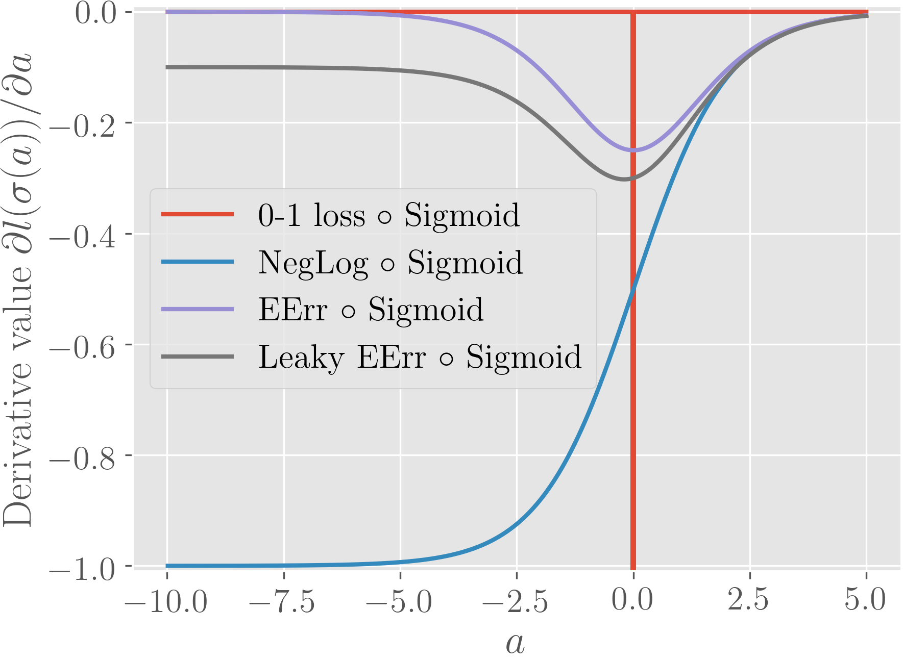 Figure 1
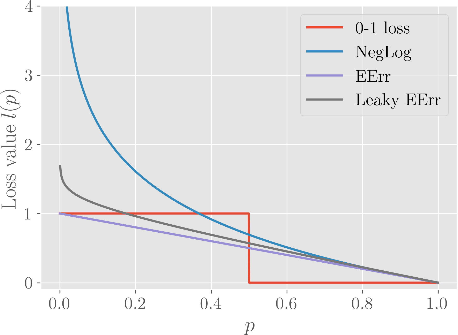 Figure 2
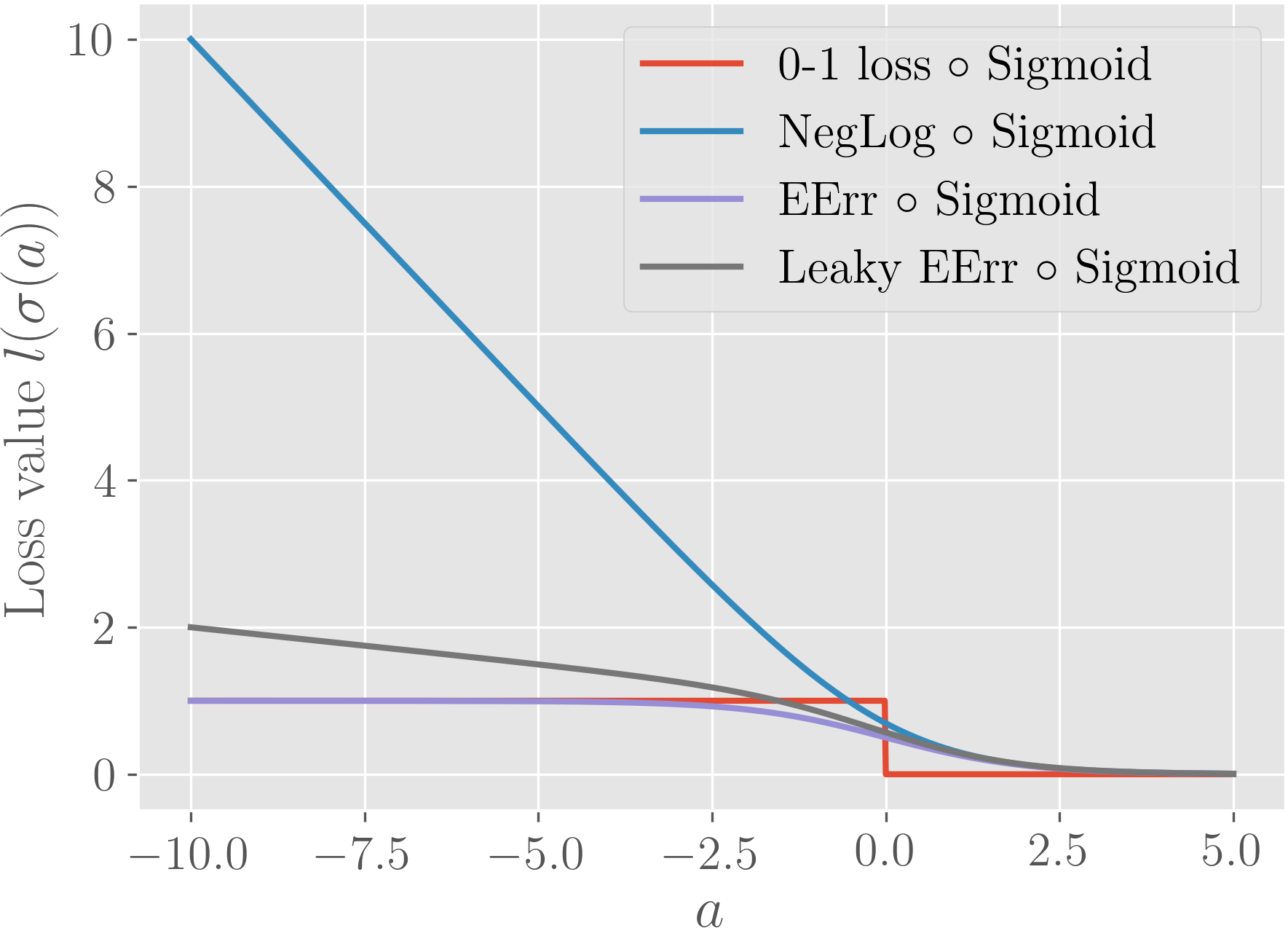 Figure 3
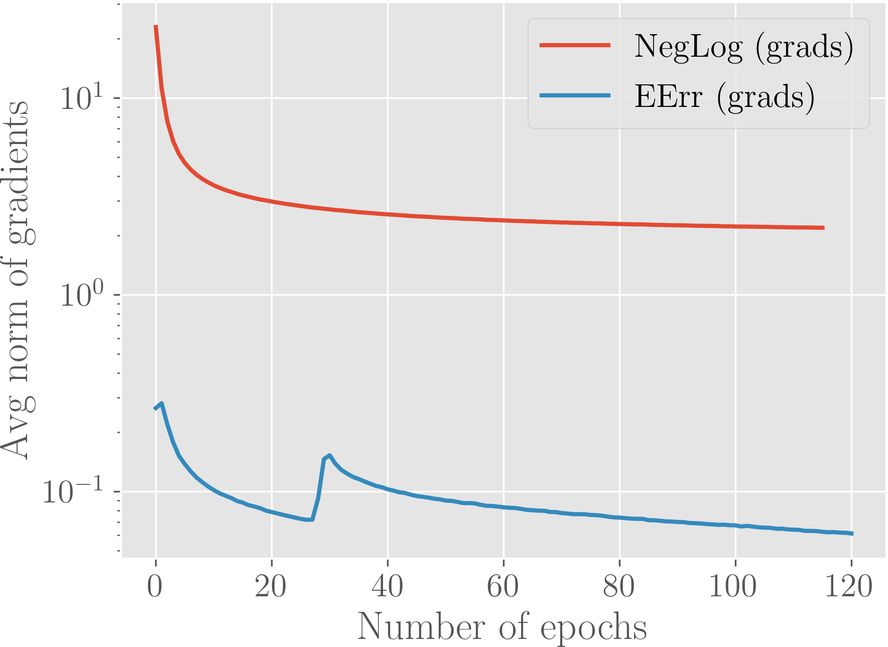 Figure 4
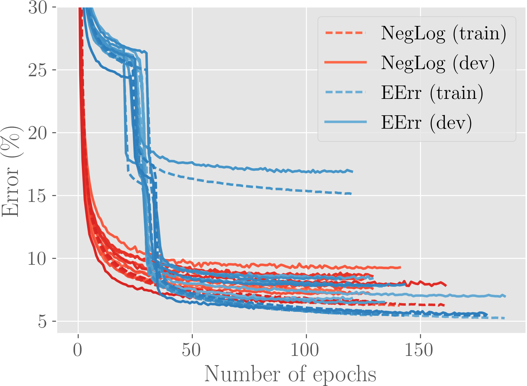 Figure 5
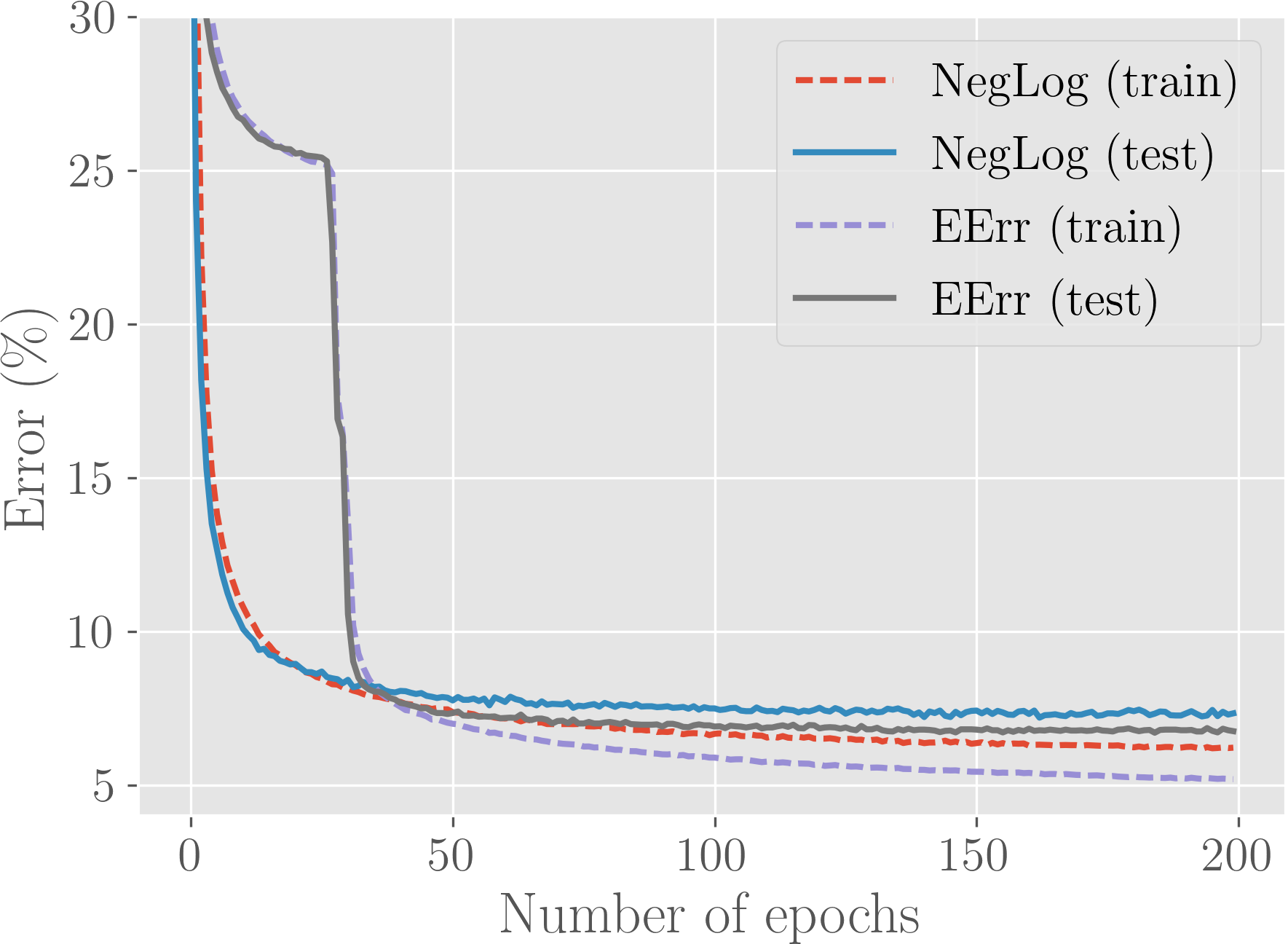 Figure 6
| Data | Instances | Dims | Classes |
|---|---|---|---|
| magic | 19020 | 10 | 2 |
| musk2 | 6598 | 166 | 2 |
| pima | 768 | 8 | 2 |
| polyadenylation | 6371 | 169 | 2 |
| ringnorm | 7400 | 20 | 2 |
| satellite47 | 2134 | 36 | 2 |
| Data |
|
Dims | Classes | ||
|---|---|---|---|---|---|
| MNIST | 70000 | 28 28 | 10 | ||
| CIFAR10 | 60000 | 32 32 3 | 10 | ||
| PTB | 49208 | - | 45 | ||
| CoNLL03 | 22137 | - | 9 | ||
| SSTB | 11855 | - | 5 |
| Data | NegLog | EErr | LEErr |
|---|---|---|---|
| magic | 20.84 0.26 | 20.54 0.27 | 20.52 0.18 |
| musk2 | 5.84 0.64 | 5.41 0.36 | 5.21 0.53 |
| pima | 23.54 1.41 | 25.06 2.14 | 23.50 0.91 |
| polya | 22.66 0.38 | 23.35 0.55 | 22.82 0.30 |
| ringn | 23.48 0.23 | 22.67 0.41 | 22.78 0.28 |
| sat47 | 16.74 0.80 | 16.21 0.56 | 16.49 0.88 |
| Data | NegLog | LEErr |
|---|---|---|
| MNIST | 1.49 0.08 | 1.40 0.08 |
| MNIST* | 1.77 0.08 | 1.61 0.08 |
| Data | NegLog | LEErr |
|---|---|---|
| CIFAR10 | 92.20 0.25 | 92.39 0.20 |
| Data | NegLog | LEErr |
|---|---|---|
| PTB | 96.82 0.05 | 96.95 0.03 |
| CoNLL03 | 97.36 0.06 | 97.37 0.07 |
| CoNLL03* | 97.12 0.12 | 97.37 0.06 |
| Data | NegLog | LEErr |
|---|---|---|
| SSTB (sent) | 48.94 0.82 | 48.55 0.80 |
| SSTB (phrase) | 82.11 0.09 | 82.03 0.13 |
Peer Reviews
No public reviews on file for this paper yet. If you reviewed it on a platform where reviews are public (OpenReview, ICLR, NeurIPS, ICML), you can paste yours below so the community can read it here.
Videos
No videos yet. Explain this paper in a talk, walkthrough, or lecture? Add one.
Taxonomy
TopicsAdversarial Robustness in Machine Learning · Anomaly Detection Techniques and Applications · Machine Learning and Data Classification
MethodsSoftmax
On Expected Accuracy
Ozan İrsoy
Bloomberg L.P.731 Lexington AveNew YorkNY10022
(2019)
Abstract.
We empirically investigate the (negative) expected accuracy as an alternative loss function to cross entropy (negative log likelihood) for classification tasks. Coupled with softmax activation, it has small derivatives over most of its domain, and is therefore hard to optimize. A modified, leaky version is evaluated on a variety of classification tasks, including digit recognition, image classification, sequence tagging and tree tagging, using a variety of neural architectures such as logistic regression, multilayer perceptron, CNN, LSTM and Tree-LSTM. We show that it yields comparable or better accuracy compared to cross entropy. Furthermore, the proposed objective is shown to be more robust to label noise.
††journalyear: 2019
1. Introduction
Classification is perhaps the most prominent supervised learning task in machine learning (Alpaydin, 2009). In classification, we are interested in assigning a given instance to a set of predetermined categories, based on prior observations in our training data. Typically, in classification, we use the maximum likelihood approach to estimate model parameters (Vapnik, 2013; Millar, 2011). In this approach, we aim to find the most likely model parameters that could explain the observations in our training set. This leads to the popular negative log likelihood objective function. However, there is an established mismatch in preeminent approaches: Even though we optimize for the negative log likelihood, we still compare models on their (test) accuracy, or error rate (Kotsiantis, 2007; Weiss and Kapouleas, 1990; Krizhevsky and Hinton, 2009; Nair and Hinton, 2010). This leads us to ask: why not optimize for accuracy directly? A simple answer would be that it is not differentiable, since it is not even continuous at the decision boundary. Another reason might be the desirable properties of the likelihood approach: if the true class label is probabilistic given by a joint distribution of instances and labels, the likelihood objective would converge to the actual distribution, given enough data (Kiefer and Wolfowitz, 1956; Banker, 1993). Still, in most settings we might actually only care about accuracy and think of log likelihood as a surrogate function to it (Witten et al., 2016). A mistake might have the same cost regardless of how close it is to the decision boundary.
This is certainly not a new question. Prior work has investigated the notion of a surrogate loss function that upper bounds the 0-1 loss, with the assumption that, optimizing the surrogate risk results in a better true risk (Pires and Szepesvári, 2016; Bartlett et al., 2006). Alternatively, margin based loss functions such as the hinge loss in support vector machines provide alternatives to the probabilistic log likelihood approaches (Wu and Liu, 2007; Wahba et al., 1999; Lin, 2004). Other work investigates the Fischer-consistent loss functions (proper scoring rules), such as squared error loss or boosting loss (Buja et al., 2005).
In this work we investigate a very simplistic loss function: negative expected accuracy (or error rate). We show that even though we define the expectation over the model distribution rather than the data distribution, this still gives us a loss function that is close to the actual accuracy (or 0-1 loss). We subsequently see that this particular loss function introduces difficulty in its optimization, and therefore further explore a leaky version of it. In a variety of experiments that cover a wide range of architectures and settings, we compare it to the traditional log likelihood loss and examine its strengths.
In Section 2, we provide the rigorous formulation of the expected accuracy and the leaky expected accuracy. In Section 3.1, we perform preliminary experiments that compare different loss functions. Based on these preliminary results, in Section 3.2 we lay out the further experimental setting and in Section 3.3 we present the main experimental results. Finally, we present our conclusions in Section 4.
2. Methodology
Consider a classification setting where a prediction function assigns a categorical distribution , to an input instance , and the final class assignment is done randomly by sampling a class label from :
[TABLE]
This is slightly different than the traditional setting where the most likely class is picked (). However since exact accuracy would be discontinuous, the stochastic setting allows us to define a continuous and differentiable proxy.
Given a dataset of instance - true label pairs , the expected accuracy of the prediction function would be:
[TABLE]
This is simply the sum of all probabilities assigned to the correct class labels (up to a constant factor of ).
We can negate this quantity to turn into a loss function (-). We can additionally translate it to get the expected error rate ((1-)), which would yield the same objective up to a constant additive factor.
2.1. Comparison to negative log likelihood
Negative expected accuracy as defined above looks similar to negative log likelihood except that we sum the probabilities themselves rather than their logs. Both loss functions optimize for high probability values assigned to the correct class, but weighted differently.
Surrogate for the 0-1 loss. If we look at the task of classification from an optimization point of view, we can describe the approach as follows:
- (1)
Our main goal is to optimize for the test set accuracy. 2. (2)
Since we cannot optimize over unseen data, we settle for optimizing for the training set accuracy and hope to have good test set accuracy as a side effect. 3. (3)
Since we cannot optimize for accuracy using a gradient-based method (due to its nondifferentiability), we settle for optimizing a differentiable surrogate function that approximates it well enough.111There is an argument that a better training objective surrogate (or even the exact accuracy) could be worse for test accuracy. We discuss this in the final section.
In this regard, we can compare both losses with respect to the 0-1 loss (error rate for a single instance) as a function of the probability value assigned to the true class label. We visualize the functions in Figure 1 (a). Negative log likelihood diverges from 0-1 loss as we approach 0. It values an increase in probability values (of the true class), say, from 0.1 to 0.2 more than an increase from 0.45 to 0.55, whereas both would be similar for the expected accuracy. We posit that instead of prioritizing correction of those instances that we perform very poorly on, by weighing probability errors equally, we might just be able to push more instances to the other side of the decision boundary. Note that in the cases that we can perform well on the training set for the negative log likelihood, both functions behave similarly.
As functions of pre-activations. Commonly the softmax activation (or sigmoid in the binary classification case) is used to convert unbounded scores (pre-activations) to probability values. We can consider the composition of loss functions and the softmax as a function of these pre-activations , which gives us another view. We visualize the compositions as such in Figure 1 (b).
Logarithm and the exponential within sigmoid cancel each other asymptotically for -log(sigmoid()) for negative values of . This approximately linear behavior allows it to have (absolutely) large derivatives () which is desirable for its optimization. On the other hand, expected error rate, coupled with the sigmoid has an asymptotically zero derivative around the negative region, which potentially make it hard to optimize. For the instances that we are the most incorrect on, progress could be very little. Still, the main motivating idea behind it is to provide more incentive (larger absolute derivatives) over the instances that are closer to the decision boundary, to grab the lower hanging fruit first.
As we will see in the later sections, difficulty of optimizing the negative expected accuracy will indeed present itself as a practical issue. To combat this, we explore a leaky version of it, by combining it with the traditional log likelihood function:
[TABLE]
for some small value of . We use in this work. As seen in Figure 1, this gives us a similar curve while having a nonzero asymptotic derivative in the negative region.
Bayes optimal predictors. In general, in classification we assume the true label of an instance is a random variable rather than a deterministic value, since is assumed to be from a joint distribution. Negative log likelihood objective has the desirable property that the predicted conditional distribution converges to the true distribution as we have more observations. This does not hold for the expected accuracy. In fact the Bayes optimal predictor for it is to assign a one-hot probability distribution which marks the most likely class. Maximum likelihood approach strives for matching the predicted and true distributions of labels, where expected accuracy wants to simply improve the counts for matching class predictions. Since from an accuracy perspective the best label that we can predict is the one that has the most instances in the population, such a Bayes optimal predictor is intuitive for its objective.
Noisy labels. Since negative likelihood diverges the most from 0-1 loss in the most negative region, we hypothesize that the impact of the proposed alternative will be the most apparent in the noisy label setting where each instance has a probability of its label being flipped. This setting simulates practical issues such as annotation errors.
3. Experiments
3.1. Preliminary Experiments
For preliminary experimentation, we use the logistic regression method over the MNIST digit recognition dataset, which has 60k train and 10k test instances of digits which are of 2828 dimensional. The task is to classify each digit into one of the ten classes. We train the model over 200 epochs using the Adam update rule (Kingma and Ba, 2014) with a learning rate of 1e-4.
Results are given in Figure 2 as training and test curves. We see that in terms of both training and test performance, expected accuracy performs better. However, as we suspected, we observe a temporary plateauing of performance in the early stages of training for the expected accuracy.
To account for randomness, and investigate consistency of the behavioral patterns, we perform 10-fold cross-validation by splitting the entire training set into training-development partitions of ratio 9:1. Development set is used for early stopping for a patience value of 15 epochs.
Results for the replicated experiments are given in Figure 3. We observe that initial plateauing is consistent across different runs. Furthermore, even though we see good performance compared to negative log likelihood for many runs, there is a particular run that the expected accuracy cannot overcome the initial plateau, resulting in a suboptimal performance by a wide margin.
Magnitudes of gradients. A possible culprit that would explain the early plateauing is simply the low magnitudes of gradients for the loss function of interest. We plot the average norms of the gradients of both losses (composed with the softmax) with respect to the softmax pre-activations in Figure 4 for one of the runs.
As we confirm a two order of magnitude difference in the norms, we rerun the experiments with a learning rate of 1e-2 for the negative expected accuracy loss, since merely having a larger learning rate might resolve getting stuck early on. However we observe a behavior that is very similar to Figure 3 (henceforth, the plot is ommitted), which confirms that the issue is more fundamental. This justifes the use of the leaky expected accuracy as defined in Equation 6 as a simple workaround.
3.2. Main Experimental Setting
Architectures. For further experiments we explore several classification related tasks using various architectures:
- •
Multilayer perceptron (MLP). We use a three hidden layer feedforward neural network with ReLU activations (Nair and Hinton, 2010). Number of hidden units are set to 300, 200 and 100 for each layer respectively. We use dropout regularization for both the input as well as the hidden layers in which we randomly drop each unit with probability (Srivastava et al., 2014).
- •
Convolutional neural network (CNN). As a CNN we use the ResNet18 deep residual network architecture (He et al., 2016). To combat overfitting, we provide small random translations or horizontal flips of each training image to the network.
- •
Bidirectional LSTM. For sequence tagging tasks, we use a bidirectional long short-term memory architecture (Hochreiter and Schmidhuber, 1997; Schuster and Paliwal, 1997). We use 100 hidden units / memory cells in each direction.
- •
Tree LSTM. For tree tagging (e.g. sentiment classification over parse trees of sentences) we use a tree LSTM architecture (Tai et al., 2015) which generalizes the traditional LSTM such that it can operate over tree structures. Again, we fix the number of hidden units to 100.
For architectures that operate over textual data, we represent each word using a dense word embedding. To this end, we use the pretrained 300-dimensional Glove word embeddings (Pennington et al., 2014).
Data. For logistic regression, we use six relatively small datasets from the UCI repository (Dheeru and Karra Taniskidou, 2017): magic (Bock et al., 2004), musk2 (Dietterich et al., 1994), pima (Smith et al., 1988), polyadenylation, ringnorm (Breiman, 1996), satellite47. Number of instances, dimensionality and number of class labels for each dataset are shown in Table 1.
For the MLP architecture, we use the MNIST dataset which we used for our preliminary experiments.
For the CNN architecture (ResNet) we use the CIFAR10 dataset which poses an image classification task, where each 32323 image is to be classified into one of the ten categories (Krizhevsky and Hinton, 2009).
For sequence tagging tasks (in which we use the LSTM architecture), we focus on part-of-speech tagging (POS) and named entity recognition (NER) (Huang et al., 2015). We use Penn Treebank (PTB) dataset (Marcus et al., 1993) for POS and CoNLL 2003 dataset (Tjong Kim Sang and De Meulder, 2003) for NER.
For tree tagging, we use the Stanford Sentiment Treebank (SSTB) (Socher et al., 2013). SSTB includes a supervised sentiment label for every node in the binary parse tree of each sentence. Therefore, not only the sentences but every possible phrase within a sentence is labeled with a sentiment score.
See Table 2 for a breakdown of the datasets.
For a subset of the data, we also experiment in the noisy label setting where we randomly assign random labels (with a probability of 0.05) to each instance in the training and development sets. Noisy versions of the dataset are denoted with an asterisk in the results.
Learning. For each task, we use the Adam update rule (Kingma and Ba, 2014) and Xavier random initialization of parameters (Glorot and Bengio, 2010). Since batching is nontrivial, for Tree LSTM (over SSTB), we use the purely online setting of stochastic gradient descent (SGD), whereas for every other task we use minibatched training. For all tasks we perform early stopping, i.e. we pick the best iteration out of all epochs based on the development set performance. Additionally, we tune the learning rate (and dropout rate when appropriate) over the same development set. For logistic regression, we use a minimum number of 100 epochs after which we start applying an 15 epoch patience rule (a lack of improvement for 15 epoch over the development set ends the run). This is because logistic regression is the least costly method and the datasets are small. For MLP and LSTMs, we apply a 30 epoch patience with no minimum or maximum number of epochs. For CNNs and Tree LSTMs, we apply 200 epochs without a patience value. These hyperparameters are intentionally left different to cover a wider range of settings.
Replication. For purposes of replication and to account for extraneous randomness such as data splits, initialization, or the order of instances in SGD, we perform cross-validation (CV). After the original test set is left apart, we randomly split the remaining data into training and development partitions. For MNIST and CIFAR, we use 10-fold CV (there is no development partition readily available). For PTb and SSTB we first combine the original training and development partitions into a bigger set and then apply 5-fold CV, by respecting the original training and development set sizes of each dataset. For UCI datasets, we apply 52-CV, which simply reapplies 2-fold CV five times. The only exception to cross-validation is the CoNLL03 data: Since training / development / test partitions are temporally ordered, shuffling and resplitting is not possible. For this data we replicate 5 different random initializations over the same partition.
Finally, we report average accuracy / error rates (with standard deviations) over the test set and compare them using the paired t-test.
3.3. Main Experiments
Logistic regression experiments using the UCI datasets are shown in Table 3. We report mean error rate with the standard deviation across replications. Best results, as well as the ones that perform no worse than the best results in a statistically significant fashion are shown underlined (). Comparing leaky expected error (LEErr) and negative log likelihood (NegLog), we see three wins for LEErr (magic, musk2, ringnorm) and three ties (pima, polyadenylation, satellite47). We see that LEErr consistently performs best (or no worse that best). Unmodified expected error rate (EErr) has four instances in which it is no worse than the best, however for two datasets, it is significantly worse than the other two (pima, polyadenylation). For later experiments we omit EErr.
Table 4 lists the results for the MLP architecture using MNIST. We observe that LEErr outperforms NegLog by a slight but (statistically) significant margin. When we rerun the experiment using the noisy label case (denoted as MNIST*), we observe a similar result with an increase in the margin. This is in line with our hypothesis about the differences of the two function possibly being more noticeable in the noisy labeling setting since more instances will lie in the negative region.
ResNet18 results over CIFAR10 are presented in Table 5. For this setting, we observe no discernible difference with the two approaches. On average, LEErr performs about single standard deviation better than NegLog, however the difference is not statistically significant.
Results for sequence tagging using bidirectional LSTMs are given in Table 6. For part-of-speech tagging over PTB, we see a statistically significant improvement using LErr (96.95 vs 96.82). For named entity recognition over CoNLL03 however we see a very close tie. When we inject noise to the labels, there is no degradation for LErr (the test accuracy stays at 97.37) whereas NegLog drops from 97.36 to 97.12. In that setting, the difference between NegLog and LEErr is significant.
Finally, results for sentiment classification over binary parse trees are demonstrated in Table 7. Since the data contains sentiment labels all phrases (all tree nodes) as well as sentences (only root nodes), we can evaluate the accuracy for both. For both measurements we see a tie: LEErr performs slightly worse than NegLog, however the difference is not significant.
4. Conclusion and Future Work
We experimentally investigate the expected accuracy / error rate (and in particular, its leaky version) as an alternative classification objective over a number of architectures and tasks. For some settings, we observe improvements over log likelihood, such as logistic regression, multilayer perceptron and sequence tagging with RNNs. For others, it performs comparably, e.g. for CNNs and Tree LSTMs. We find the results promising since LEErr overall performs better or no worse than NegLog.
One of the main motivations behind expected accuracy is to provide a more faithful approximation to accuracy. However there is a chance that optimizing for training accuracy (or expected accuracy) to be worse for generalization accuracy. For instance, this is an argument for the margin based loss approaches, since having a large margin around the decision boundary tends to improve generalization (even though accuracy itself does not have any margin) (Lin, 2004). In this work, we compare loss functions over the test set to ensure that their generalization performance is evaluated.
Log likelihood is perhaps the most commonly used probabilistic objective for classification, and is well studied. Many of the recent innovations in deep learning that led to being able to train better models, such as improved regularization (Srivastava et al., 2014), better activation functions (Nair and Hinton, 2010), or improved update rules (Kingma and Ba, 2014) are studied using the cross entropy classification objective, therefore expected to synergize well with it. Similarly, recent results on loss surfaces or convergence dynamics of neural networks use softmax with log likelihood losses (Li et al., 2018; Li and Yuan, 2017). We believe that future work that uses the (leaky) expected accuracy objective could discover more compatible hyperparameters with improved performance.
The reference list from the paper itself. Each links out to its DOI / PubMed record.
- 1(1)
- 2Alpaydin (2009) Ethem Alpaydin. 2009. Introduction to machine learning . MIT press.
- 3Banker (1993) Rajiv D Banker. 1993. Maximum likelihood, consistency and data envelopment analysis: a statistical foundation. Management science 39, 10 (1993), 1265–1273.
- 4Bartlett et al . (2006) Peter L Bartlett, Michael I Jordan, and Jon D Mc Auliffe. 2006. Convexity, classification, and risk bounds. J. Amer. Statist. Assoc. 101, 473 (2006), 138–156.
- 5Bock et al . (2004) RK Bock, A Chilingarian, M Gaug, F Hakl, Th Hengstebeck, M Jiřina, J Klaschka, E Kotrč, P Savickỳ, S Towers, et al . 2004. Methods for multidimensional event classification: a case study using images from a Cherenkov gamma-ray telescope. Nuclear Instruments and Methods in Physics Research Section A: Accelerators, Spectrometers, Detectors and Associated Equipment 516, 2-3 (2004), 511–528.
- 6Breiman (1996) Leo Breiman. 1996. Bias, variance, and arcing classifiers. (1996).
- 7Buja et al . (2005) Andreas Buja, Werner Stuetzle, and Yi Shen. 2005. Loss functions for binary class probability estimation and classification: Structure and applications. Working draft, November 3 (2005).
- 8Dheeru and Karra Taniskidou (2017) Dua Dheeru and Efi Karra Taniskidou. 2017. UCI Machine Learning Repository. http://archive.ics.uci.edu/ml