Ricci-flat metrics on vector bundles over flag manifolds
Ismail Achmed-Zade, Dmitri Bykov

TL;DR
This paper constructs explicit complete Ricci-flat metrics on vector bundles over flag manifolds of SU(n), generalizing known metrics on conifolds and canonical bundles, expanding the class of explicit Ricci-flat geometries.
Contribution
It provides new explicit Ricci-flat metrics on vector bundles over flag manifolds, extending previous constructions to a broader class of geometries.
Findings
Explicit Ricci-flat metrics constructed
Metrics generalize known conifold and canonical bundle metrics
Applicable to all Kähler classes on the bundles
Abstract
We construct explicit complete Ricci-flat metrics on the total spaces of certain vector bundles over flag manifolds of the group , for all K\"ahler classes. These metrics are natural generalizations of the metrics of Candelas-de la Ossa on the conifold, Pando Zayas-Tseytlin on the canonical bundle over , as well as the metrics on canonical bundles over flag manifolds, recently constructed by van Coevering.
Click any figure to enlarge with its caption.
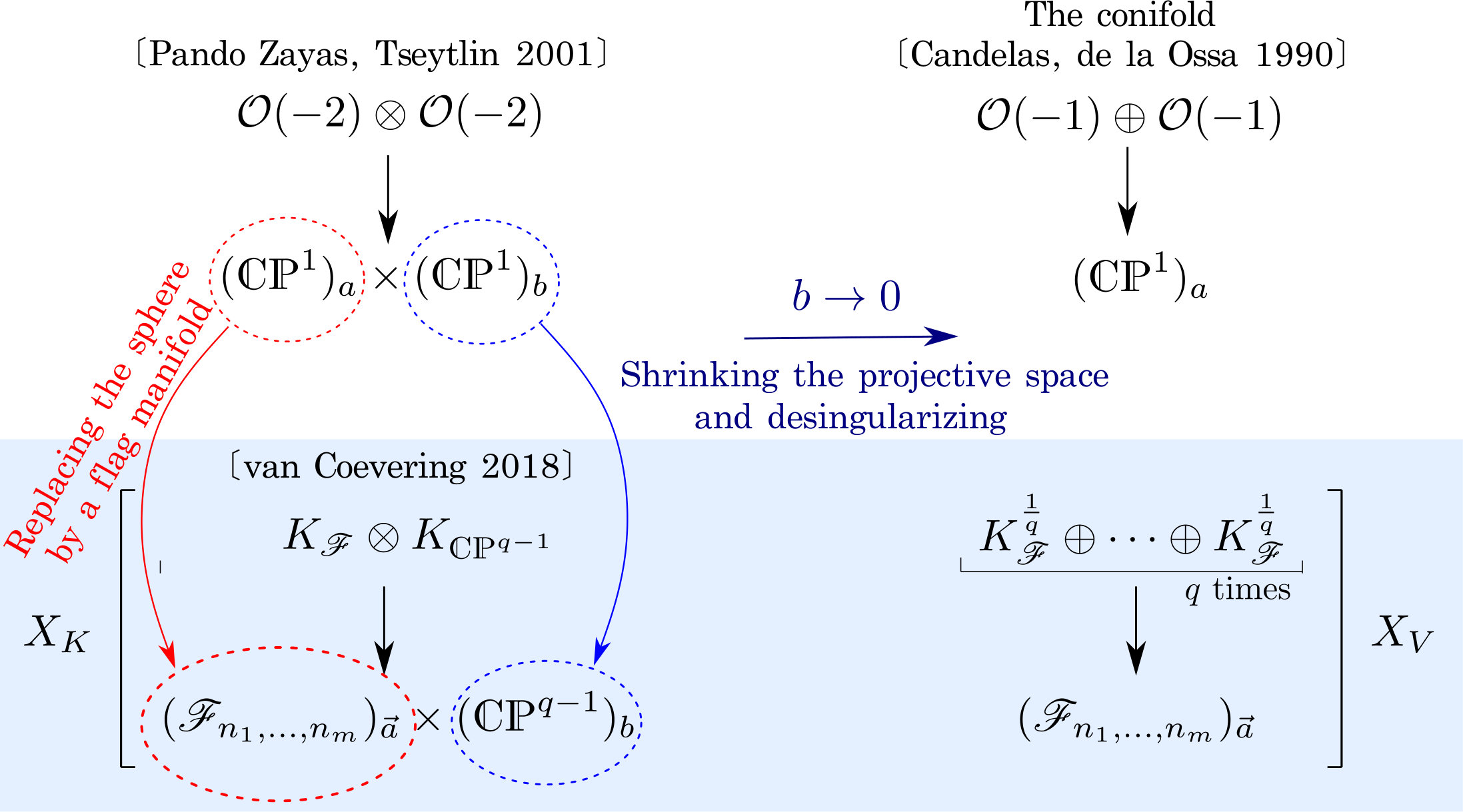 Figure 1
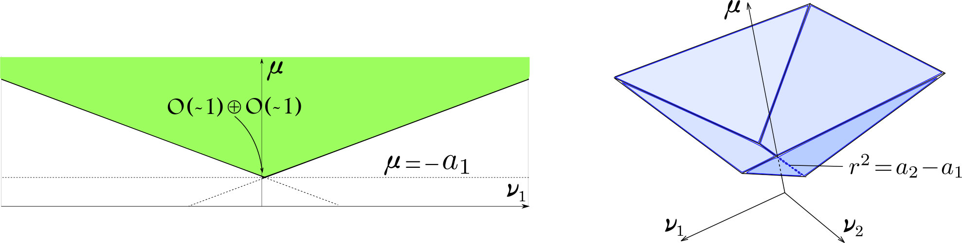 Figure 2
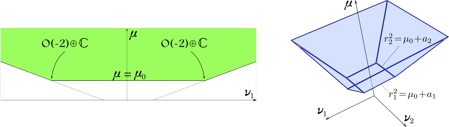 Figure 3
Peer Reviews
No public reviews on file for this paper yet. If you reviewed it on a platform where reviews are public (OpenReview, ICLR, NeurIPS, ICML), you can paste yours below so the community can read it here.
Videos
No videos yet. Explain this paper in a talk, walkthrough, or lecture? Add one.
MPP-2019-81
LMU-ASC 17/19
Ricci-flat metrics on vector bundles
over flag manifolds
Ismail Achmed-Zade1,2 and Dmitri Bykov1,2,3111Emails: [email protected], [email protected], [email protected]
1 Max-Planck-Institut für Physik, Föhringer Ring 6, D-80805 Munich, Germany
2 Arnold Sommerfeld Center for Theoretical Physics,
Theresienstrasse 37, D-80333 Munich, Germany
3 Steklov Mathematical Institute of Russ. Acad. Sci.,
Gubkina str. 8, 119991 Moscow, Russia
Abstract. We construct explicit complete Ricci-flat metrics on the total spaces of certain vector bundles over flag manifolds of the group , for all Kähler classes. These metrics are natural generalizations of the metrics of Candelas-de la Ossa on the conifold, Pando Zayas-Tseytlin on the canonical bundle over , as well as the metrics on canonical bundles over flag manifolds, recently constructed by van Coevering.
Contents
1 Introduction and main result
The problem of constructing explicit Ricci-flat Kähler metrics is rather complicated. In the compact case no such metrics are known, due to the fact that the condition of Ricci-flatness implies the absence of non-parallel Killing vectors [1, Section 1.84]. However, in the non-compact case symmetries may be present, and the metrics are sometimes known in explicit form. The early examples include the Eguchi-Hanson ‘gravitational instanton’ [2] and its generalizations by Gibbons and Hawking [3]. Another example that will be important for us is the metric of Candelas-de la Ossa [4] on the so-called ‘resolved conifold’ and its immediate generalization constructed in [5]. Various other metrics are known: those of cohomogeneity one of Stenzel [6] and Nitta [7] as well as the higher-cohomegeneity metrics on manifolds that admit Killing-Yano tensors [8, 9]. One can also construct hyperkähler metrics on the cotangent bundle of flag manifolds using the hyperkähler quotient construction of [10]. In the simplest case of the Grassmannians this was elaborated upon in [11]. For the purposes of the present paper, however, it will be sufficient to understand in detail the examples of [2, 4, 5].
An important feature of the metric of [2] is that it may be thought of as the metric on the total space of the canonical bundle over . In fact, it is a simple application of the so-called Calabi ansatz [12], which allows constructing a complete Ricci-flat metric on the canonical bundle of a Kähler-Einstein manifold of positive curvature – in this case this manifold is simply with its Fubini-Study (round) metric.
An interesting generalization may be obtained by replacing the base manifold by a manifold of flags in . We recall that a flag manifold may be specified by a sequence of increasing integers which define the flag
[TABLE]
where are linear subspaces of , such that . In place of we will often use the integers , defined by . In these terms, the manifold of flags (1.1) is a homogeneous space
[TABLE]
In what follows we will sometimes use the short notation for this manifold. The complex geometry of flag manifolds was first studied in the classical work [13].
The authors of [14] use Calabi’s ansatz to construct a Ricci-flat metric on the canonical bundle of the flag manifold, equipped with such a Kähler-Einstein metric. An important characteristic of Calabi’s ansatz, that we review in Section 2, is that it produces a metric with a fixed Kähler class. On the other hand, by the Calabi-Yau theorem [15, 16, 17], in the case of a compact manifold with there should exist a Ricci-flat metric in every Kähler class. The relevant non-compact generalization of the theorem (to asymptotically-conical spaces), with the same statement, was constructed in [18, 19].
The Kähler cone of the total space of the canonical bundle over the flag manifold is the same as that of the underlying flag manifold. The Kähler moduli of the flag manifold, in turn, can be easily characterized geometrically:
- •
As parameters defining an adjoint orbit, in which case the Kähler form is the Kirillov-Kostant form on this orbit (see [20] for a review).
- •
As Fayet-Iliopoulos parameters related to the gauged linear -model representations for flag manifolds [21, 22].
- •
The most general Kähler metric can be directly constructed using the so-called quasi-potentials [23, 24] that also featured in the physics literature in [25]. We will adopt this strategy throughout the paper.
As a result, for the -step flag manifold (i.e. for the flags of type (1.1)) there are real moduli. Therefore Calabi’s ansatz does not capture the full moduli space of Ricci-flat metrics on the total space. This was taken into account in [26], where a full family of Ricci-flat metrics on the total space of was constructed, using a generalization of Calabi’s ansatz. In fact, this generalization is analogous to the one that arose in the work [4] on the conifold and was also considered in [7].
Another interesting analogy may be observed, if one adds to the above the work [5], where essentially the Ricci-flat Kähler metric on the total space of was constructed. As required by the Calabi-Yau theorem, this metric has two Kähler moduli (since ), which geometrically correspond to the radii of the two spheres representing the ‘zero section’. As one of the spheres shrinks (i.e., as we approach the boundary of the Kähler cone in a particular way), one gets a metric on a bundle over . Such orbifold bundles were investigated in a more general context in [27]. Removing the orbifold singularity at the zero section, one obtains the total space of the vector bundle over [4] (the so-called ‘conifold’).
In the present paper we pursue a suitable generalization of this procedure to flag manifolds . In this case, in place of , we start with the manifold , and construct a Ricci-flat metric on
[TABLE]
In fact, alternatively one may view the manifold as a flag manifold of a semi-simple group , which allows to identify these metrics with a special case of the metrics constructed in [26]. We then take the limit, when the volume of vanishes, remove a -orbifold singularity and show that in the special case when the line bundle is well-defined (i.e., when divides ), the resulting manifold is
[TABLE]
over . The latter rank- vector bundle will be denoted . The logic just described is summarized in Fig. 1.
To formulate our result more precisely, we recall the expression for the first Chern class of the flag manifold:
[TABLE]
where are pullbacks of tautological bundles over w.r.t. the forgetful projections . We recall the derivation of this formula in section 3.1.
We prove the following statement:
Proposition. There exists a complete Ricci-flat Kähler metric on in each Kähler class. If there exists a such that (), then there exists a complete Ricci-flat Kähler metric on in each Kähler class. In both cases the line element of the metric is of the form
[TABLE]
*where is the Fubini-Study metric on , and is the Kähler-Einstein metric, satisfying , on the Grassmannian manifolds , where . Besides, , is the holomorphic connection of and the constants determine the Kähler class.
The action of the complex structure is given by .
is of the form*
[TABLE]
*If , for all , and the angular variable takes values in (1.6)-(1.8) describe a metric on for all Kähler classes.
If for all , , and (1.6)-(1.8) describe a metric on for all Kähler classes.
The metrics so constructed are asymptotic to the Riemannian cone over the Sasaki-Einstein bundles over . For and these are the unit vector bundles of and its -th root respectively.
Comment.* We note that the line element (1.6) has the form of Pedersen-Poon [28].
The structure of the paper is as follows. In section 2 we recall, how the Ricci-flat Kähler metric on is constructed, using a generalization of Calabi’s ansatz. In section 3 we pass over to flag manifolds, starting in section 3.1 by explaining the expression for the first Chern class of a flag manifold and constructing the Kähler-Einstein metric in explicit form. Using the Kähler-Einstein metric, we construct in section 3.2 a generalization of Calabi’s ansatz, which allows obtaining the Ricci-flat metric in every Kähler class. This generalized ansatz leads to an ODE, which is then solved in section 3.2. In the same section the topology of the manifold (the behavior near the zero section, as well as at infinity) is also analyzed. The appendix is dedicated to the calculation of the determinant of the Hermitian metric, which is used in writing out the Ricci-flatness equation.
2 Conifold and canonical bundle over
The ansatz of Calabi may be succintly formulated as the requirement that the Kähler potential on the total space assumes the form
[TABLE]
where is the Kähler potential of the Kähler-Einstein metric on the underlying manifold and is the coordinate in the fiber. Throughout the paper we will assume that the Kähler-Einstein metric on the base is normalized so that
[TABLE]
In this section as our principal example we will take . Note that this manifold has two Kähler moduli (the sizes of the two spheres), so this is the simplest instance of the situation described in the introduction, namely the Calabi-Yau theorem requires the existence of two parameters in the metric on . Calabi’s ansatz (2.1) fails to capture the full moduli space, since the Kähler-Einstein condition on requires that the radii of the two ’s be equal.
Interestingly, Calabi’s ansatz corresponds to a special point in the moduli space of metrics, namely the corresponding Kähler form lies in the compactly supported cohomology. This is characterized by a faster decay to the asymptotic form at infinity. For a more detailed discussion of this see [18, 19, 29].
Denoting the inhomogeneous coordinates on the two spheres by and , one introduces the following generalization of Calabi’s ansatz (after a simple change of variables):
[TABLE]
Clearly and are the Kähler potentials of the two spheres, and is the Kähler potential of the Einstein metric on . Setting would yield precisely the ansatz of Calabi.
Now, we are dealing with a toric variety, the holomorphic isometries being given by the rotations
[TABLE]
In such cases it is useful to pass to the moment map variables. The moment map is defined as the derivative , where is the complex structure, and is the vector field corresponding to the holomorphic isometry. In practical terms, this is tantamount to replacing , , in the Kähler potential, and differentiating it w.r.t. and :
[TABLE]
One also computes the so-called symplectic potential , which is the Legendre transform of the Kähler potential w.r.t. the variables :
[TABLE]
The nice feature of this potential is that the domain, on which it is defined, is precisely the moment polytope of the manifold. Clearly, since in our case the manifold is non-compact, the polytope is also unbounded.
Up to inessential linear terms in , the dual potential reads:
[TABLE]
Note that the structures appearing in the symplectic potential are typical for Kähler toric geometry [30]. Now, the function is determined from the Ricci-flatness equation, which in this case reads
[TABLE]
The solution is , where are the three roots of the polynomial .
Next we write down the explicit expression for the line element derived from the Kähler potential (2.3), using the dual variable :
[TABLE]
Here is the holomorphic connection on the canonical bundle . Non-negativity of the metric implies . The latter requirement is equivalent to . Note that and for , due to the first two inequalities. Completeness requires that the range of is . In fact, there are two distinct possibilities:
- •
. This was considered by Pando Zayas and Tseytlin [5].
- •
. This was considered in the early work of Candelas and de la Ossa [4].
In the first case, one has as . The change of variables brings the metric to the asymptotic form
[TABLE]
The absence of singularity at requires that the angle has the range . Then (2.11) shows that one has the canonical bundle, with connection , over , the two spheres having radii squared and . Varying leads to changing the Kähler class of the metric, and all allowed classes (corresponding to the non-vanishing sizes of the ’s) can be achieved in this way.
In the second case, let us assume that . now has a second-order zero at , so that Introducing the variable , in the vicinity of we can bring the metric to the form
[TABLE]
Here . If one sets , the expression in round brackets is precisely the round metric on , provided one takes the periodicity of the angle to be . In this case the conical part of the metric above describes the space . (Keeping instead the periodicity would lead to a orbifold singularity at the zero section, .) Taking into account the stereographic -variable of the remaining sphere , one can show that the metric (2.12) describes the vicinity of the zero section in the bundle over (the so-called ‘conifold’) [4].
Since the varieties we have considered are toric, it is instructive to construct the respective toric polytopes. The polytopes corresponding to the Pando Zayas-Tseytlin solution and the Candelas-de la Ossa solution are schematically presented in Figs. 2 and 3, respectively. The sections of the moment polytope in the plane are shown to the left of the full three-dimensional polytope.
3 Flag manifolds
In this section, apart from the unitary representation (1.2) for the flag manifold (1.1), it will be useful to recall the complex parametrization (with a parabolic subgroup, stabilizing a given flag), which expresses the flag manifold as a homogeneous space of the complex linear group .
We will start by recalling the explicit form of the Kähler-Einstein metric on the flag manifold, which is an essential ingredient in Calabi’s ansatz. We then use a suitable generalization of this ansatz to construct the metric on – the total space of the canonical bundle over , and on – the total space of the vector bundle (the latter in the case when the -th root of makes sense).
3.1 The canonical bundle
On we can consider the vector bundles and () where the fiber of over the point
[TABLE]
is given by , and the fiber of is ( are the tautological bundles). Here, as before, . As is well-known [31]
[TABLE]
We will be interested in the explicit expression for the first Chern class of the flag manifold:
[TABLE]
Rewriting in terms of gives
[TABLE]
Now, suppose there is a positive integer that divides for all . Then, since [32, Prop. 2.1.2][33], there is a line bundle , where is the canonical bundle of .
Furthermore since is Kähler we have that the Ricci-form represents . Let , where are column vectors. Then
[TABLE]
with . Therefore the line element of the Kähler-Einstein metric on , satisfying (2.2), must take the form
[TABLE]
Note that Kähler-Einstein metric on flag manifolds were first discussed in [34]. It is useful for the following discussion to write out explicitly the Kähler potential corresponding to this metric. To this end consider the matrix
[TABLE]
where each is a column vector. We also define an -matrix of rank
[TABLE]
and introduce the function
[TABLE]
One can check that is the Kähler potential for the -normalized canonical metric111The same normalization as that of the Fubini-Study metric on , i.e. the volume of a holomorphic 2-sphere generating is . on the Grassmannian . The potential of an arbitrary Kähler metric on the flag manifold [23, 24] may then be written as
[TABLE]
In particular the Kähler-Einstein metric (3.6) arises when .
3.2 Generalized Calabi Ansatz for all Kähler classes
From now on we assume there is a positive integer that divides for all . Also we define the vector .
As a candidate for a Kähler potential on , we define
[TABLE]
From the discussion in the previous section it follows that is the Kähler potential of the Kähler-Einstein metric on , and therefore the last term in (3.11) is the expression familiar from Calabi’s ansatz (2.1).
In (3.11) are the parameters (Kähler moduli), akin to from (2.3). Their range will be determined later. If we work on , the components of are local coordinates on and is a holomorphic coordinate on the fiber. If we work on , are local coordinates on the fiber.
Notice that depends only on a single variable . We will write and for its first and second derivatives w.r.t . In fact, instead of dealing with the function , just like in section (2) it is convenient to perform a Legendre transform
[TABLE]
whence
[TABLE]
The meaning of is that it is the moment map for the -action .
The line element then is given by
[TABLE]
where has the form of a Fubini-Study metric on and
[TABLE]
Note that are the complex coordinates on the flag manifold, and are abbreviations for (the components of the vectors ).
The expression (3.14) may be brought to the form (1.6) used in the statement of the Proposition, if we introduce the angular variable . Then, again using (3.24), we obtain
[TABLE]
Since , we arrive at
[TABLE]
with as covariant derivative. Since the l.h.s. of the above equality is a one-form of type , on which the complex structure acts by multiplication by , we get
[TABLE]
The -dependent part of the metric (3.14) is then
[TABLE]
We denote by the Hermitian (Kähler) metric corresponding to (3.14). The Ricci-tensor is given by where are derivatives w.r.t. the holomorphic coordinates. Therefore Ricci-flatness is satisfied if
[TABLE]
for a holomorphic function . It will be shown in App. A that
[TABLE]
where is a holomorphic function, and
[TABLE]
Using the definition
[TABLE]
from (3.11), as well as , we may satisfy (3.21) by requiring
[TABLE]
3.3 Solution of the Ricci-flatness equation
The ODE (3.25) is solved by
[TABLE]
Therefore
[TABLE]
3.3.1 Behavior at
Before analysing the effect of different choices for the integration constant , we observe that
[TABLE]
Here . Using (3.14) and (3.20) and making the substitution , we find that the line element behaves at infinity as
[TABLE]
where is the Kähler-Einstein metric on with proportionality factor . Thus at we obtain a cone over a Sasakian manifold, which is a -bundle over . As will be demonstrated in the remainder of this section the angle ranges from on and from on . Therefore the -bundles are the unit -vector bundles of and respectively.
3.3.2 The metric on
We now analyze the dependence on the choice of . If is larger than the largest root of , then is strictly positive. The only possible issue would be a singularity at the zero section, but since
[TABLE]
the substitution implies
[TABLE]
that is to say the line element corresponds to a smooth metric. The complex variable parametrizes – the fiber of a line bundle, and the connection allows to identify this bundle with . Therefore the underlying manifold is . The condition
[TABLE]
makes the metric positive-definite. Upon restricting to the zero section , (3.14) reduces to
[TABLE]
with . The definition (3.10) of the Kähler cone of the flag manifold, combined with for , implies that all Kähler classes are obtained.
3.3.3 The metric on
We will now show that for the line element (3.14) describes a metric on . Notice that positive-definiteness of the metric (3.39) requires (since for all )
[TABLE]
It then follows easily from (3.23), (3.27) that the above condition also makes (and hence the metric (1.6)) positive for .
One can visualize the limit as sending the volume of to zero and embedding into the fiber . First we notice that
[TABLE]
Since , (3.26) yields
[TABLE]
Therefore to leading order in
[TABLE]
Inserting this in the full Kähler potential (3.11) and using (3.35), we get (up to an additive constant that we forget from now on)
[TABLE]
Here we have introduced the coordinates on the fiber. They are related to via . This procedure changes the periodicity of w.r.t the metric on in complete analogy to the Pando Zayas-Tseytlin/Candelas-de la Ossa metrics discussed in section 2 (keeping the original periodicity would result in a -singularity).
As we will now see, the above formula provides a Kähler potential in the vicinity of the zero section . The zero section is given by the equations , .
Introducing the holomorphic connection , we may write out explicitly the line element corresponding to the above potential, in the limit :
[TABLE]
The second term gives a metric in the fiber of the rank- vector bundle .
At the expense of introducing a non-holomorphic complex coordinate , we may rewrite (3.38) more compactly:
[TABLE]
The absence of a conical singularity at implies that is periodic in the segment .
Acknowledgments. We would like to thank D. Lüst and A. A. Slavnov for support and D. Ageev, O. Biquard, P. Gauduchon, S. Gorchinskiy, M. Nitta, K. Shramov, P. Zinn-Justin for useful discussions. The research of I.A. was supported by the IMPRS program of the MPP Munich.
Appendix A Calculation of the determinant of the metric
The goal of this section is to compute the determinant of the Hermitian metric corresponding to the line element (3.14).
First we notice that it is easy to factor out the pieces corresponding to the -dependence of the metric, as well as to the directions. As a result we get
[TABLE]
where is the reduced Hermitian metric, with the line element
[TABLE]
This is a family of metrics on the flag manifold, depending on as a parameter. We will calculate the determinant by studying the set of values of , for which degenerates. Since the flag manifold is a homogeneous space, and the metric is a -invariant tensor, is the same at every point. To calculate it, we consider the open set in , where the matrix introduced in (3.7), which represents the quotient , may be brought to lower-block-triangular form. Evaluating at the point , we obtain:
[TABLE]
Thus
[TABLE]
The metric at is therefore diagonal, with eigenvalues being equal to , each of multiplicty . At an arbitrary point , the Hermitian metric is represented by a matrix of size , whose entries are linear in . Since , we get
[TABLE]
where
[TABLE]
and is independent of . To find , we notice that in the limit the metric (A.2) behaves as , where is the Kähler-Einstein metric on described in (3.6). Since its Kähler potential is , from we find
[TABLE]
The reference list from the paper itself. Each links out to its DOI / PubMed record.
- 1[1] A. Besse, Einstein manifolds . Springer, 2008.
- 2[2] T. Eguchi and A. J. Hanson, “Asymptotically Flat Selfdual Solutions to Euclidean Gravity,” Phys.Lett. B 74 (1978) 249 . · doi ↗
- 3[3] G. Gibbons and S. Hawking, “Gravitational Multi - Instantons,” Phys.Lett. B 78 (1978) 430 . · doi ↗
- 4[4] P. Candelas and X. C. de la Ossa, “Comments on Conifolds,” Nucl.Phys. B 342 (1990) 246–268 . · doi ↗
- 5[5] L. A. Pando Zayas and A. A. Tseytlin, “3-branes on spaces with R × S 2 × S 3 𝑅 superscript 𝑆 2 superscript 𝑆 3 R\times S^{2}\times S^{3} topology,” Phys.Rev. D 63 (2001) 086006 , ar Xiv:hep-th/0101043 [hep-th] . · doi ↗
- 6[6] M. B. Stenzel, “Ricci-flat metrics on the complexification of a compact rank one symmetric space,” Manuscripta Mathematica 80 no. 1, (1993) 151–163.
- 7[7] M. Nitta, “Noncompact Calabi-Yau metrics from nonlinear realizations,” ar Xiv:hep-th/0309004 [hep-th] .
- 8[8] V. Apostolov, D. M. Calderbank, and P. Gauduchon, “Hamiltonian 2-forms in Kähler geometry. I: General theory.,” J. Differ. Geom. 73 no. 3, (2006) 359–412.