An analysis of sparsity preserving pivot strategies for discontinuous Galerkin methods applied to acoustic scattering
Cody Lorton, Ryan Severance

TL;DR
This paper analyzes how different pivoting strategies affect the sparsity of matrices in discontinuous Galerkin methods for acoustic scattering, providing insights into reducing fill-in during LU-factorization.
Contribution
It evaluates three pivoting strategies—AMD, nested dissection, and reverse Cuthill-McKee—for their effectiveness in maintaining sparsity in IP-DG matrices.
Findings
Nested dissection best reduces fill-in.
Performance varies with mesh structure and polynomial degree.
Numerical results validate the strategies' effectiveness.
Abstract
In this paper we discuss and analyze the sparse structure of matrices associated to the interior penalty discontinuous Galerkin (IP-DG) method applied to the Helmholtz equation. It is well-known that LU-factorization causes fill-in and this paper discusses three pivoting strategies: approximate minimal degree (AMD), nested dissection, and reverse Cuthill-McKee, that can reduce fill-in associated to the LU-factorization. Numerical experiments are included that demonstrate the performance of these pivoting strategies. These experiments include both uniform and non-uniform mesh structures, the inclusion of a scattering boundary, and both piecewise linear and quadratic solution spaces.
Click any figure to enlarge with its caption.
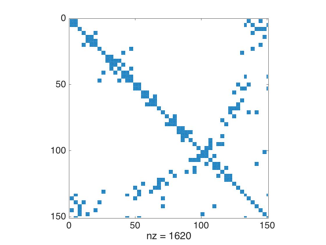 Figure 1
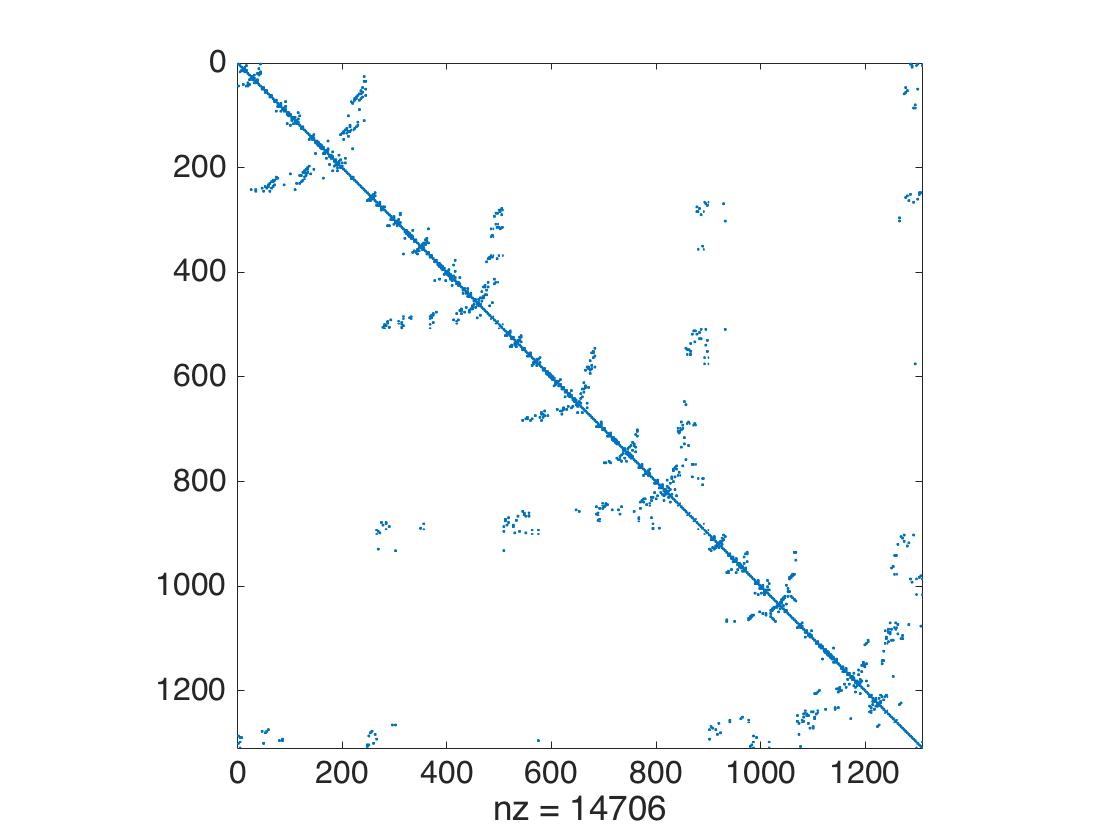 Figure 2
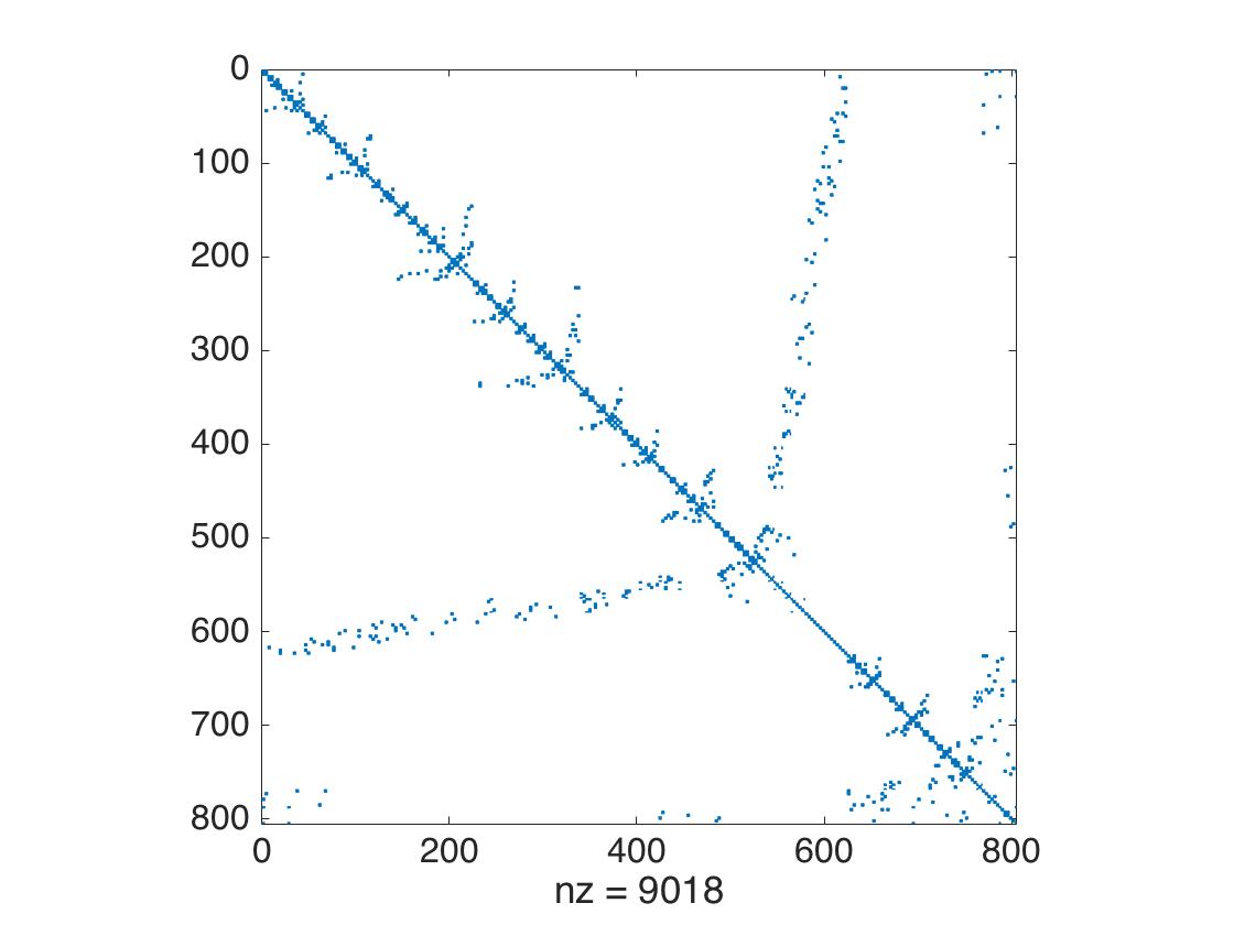 Figure 3
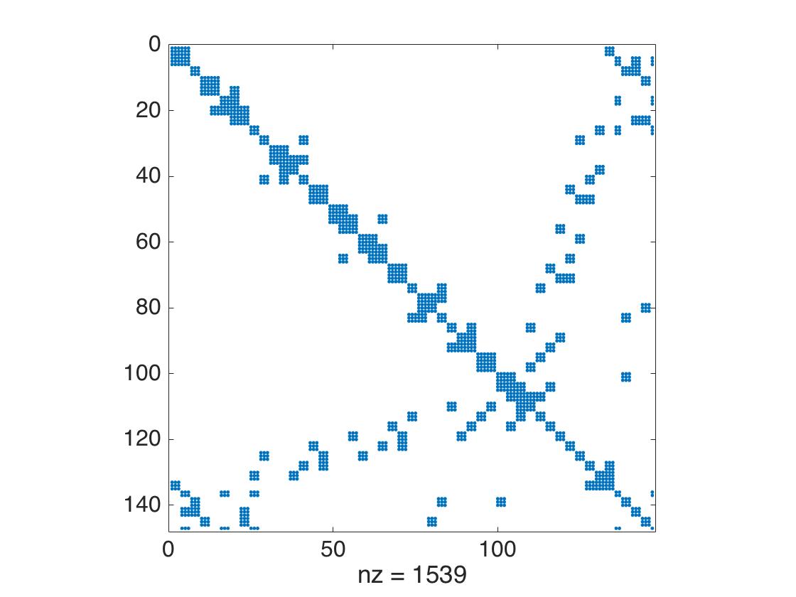 Figure 4
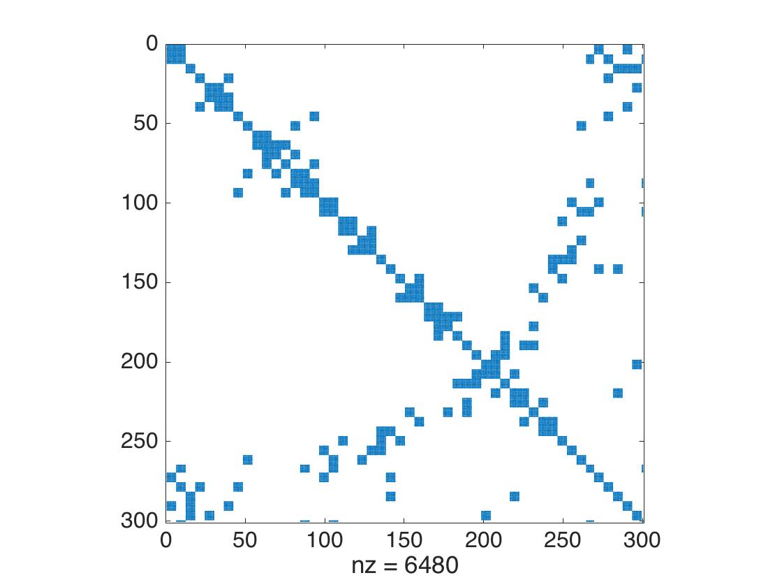 Figure 5
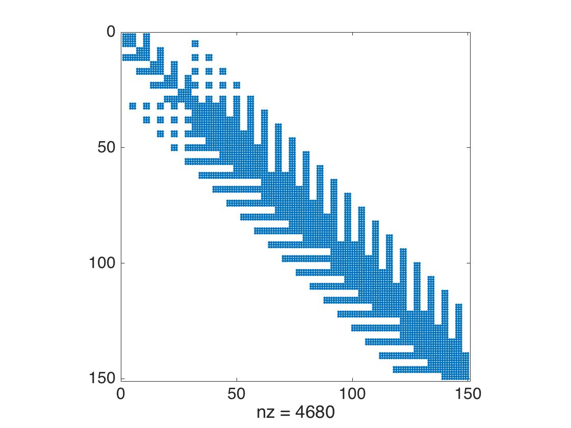 Figure 6
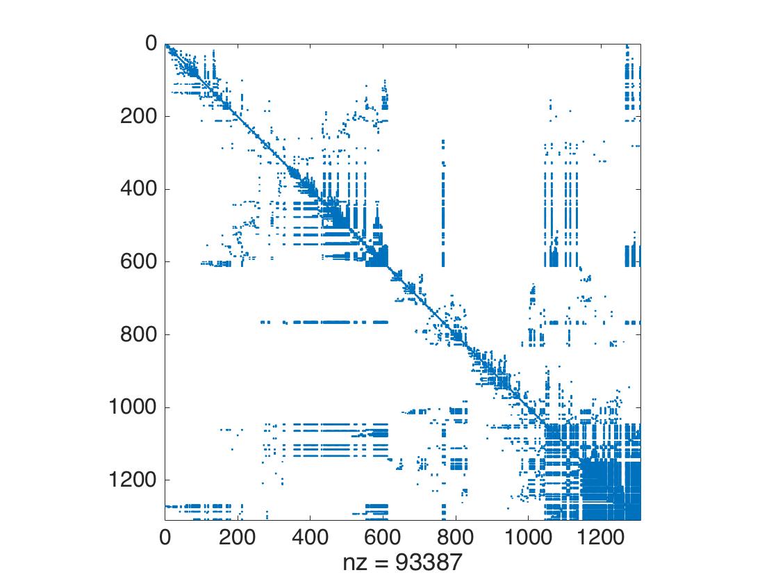 Figure 7
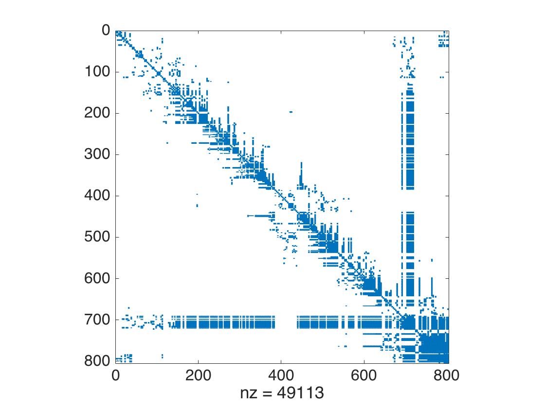 Figure 8
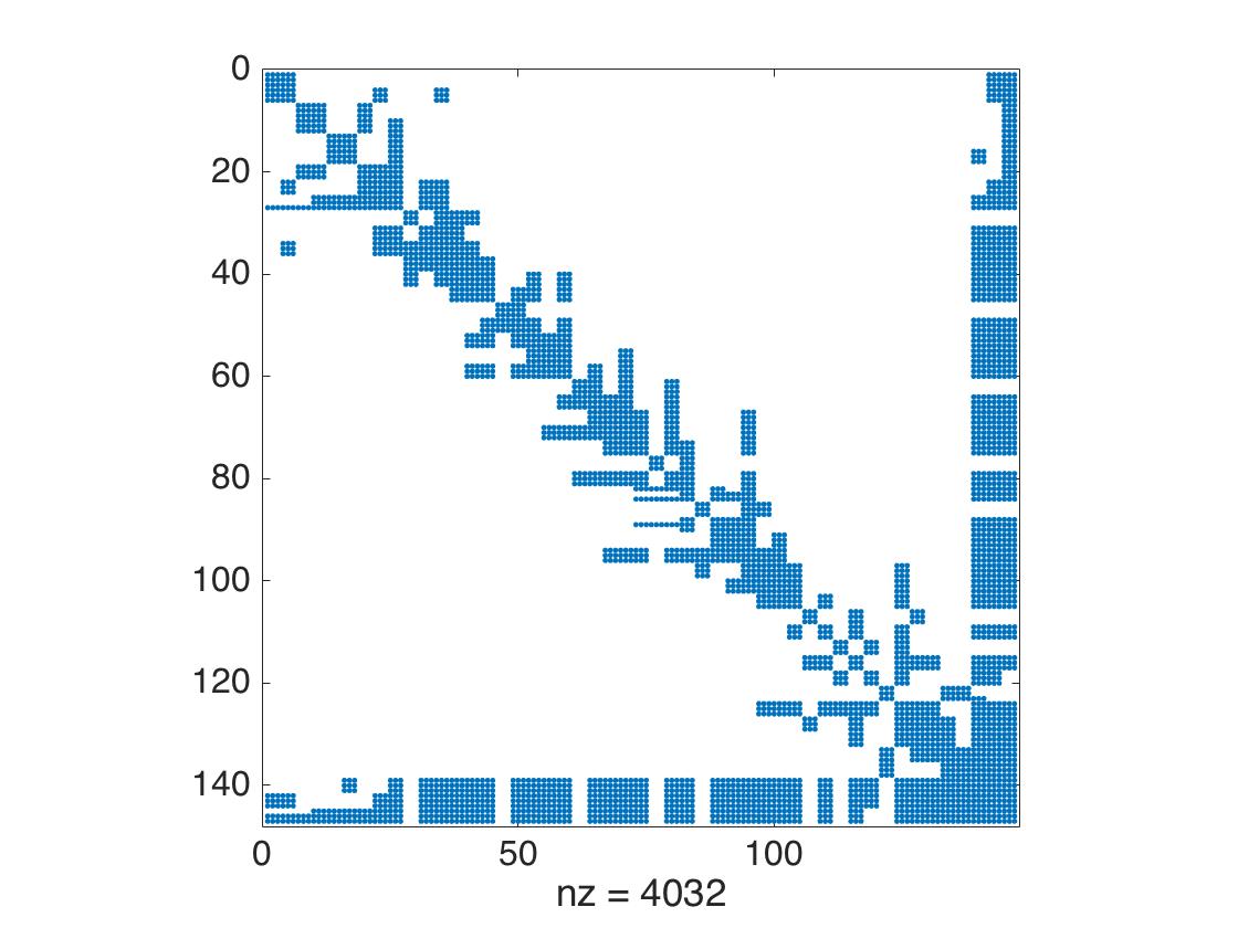 Figure 9
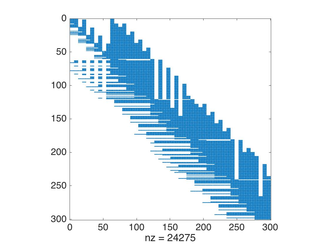 Figure 10
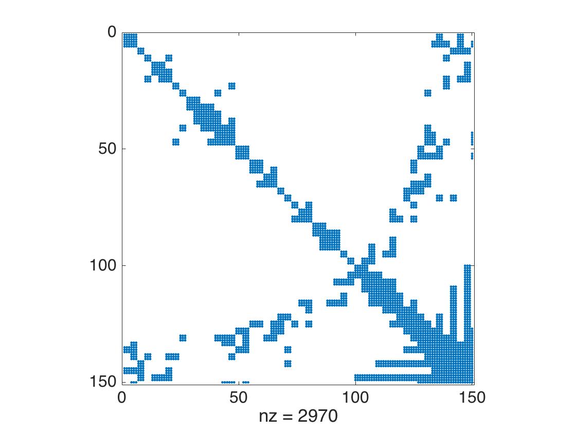 Figure 11
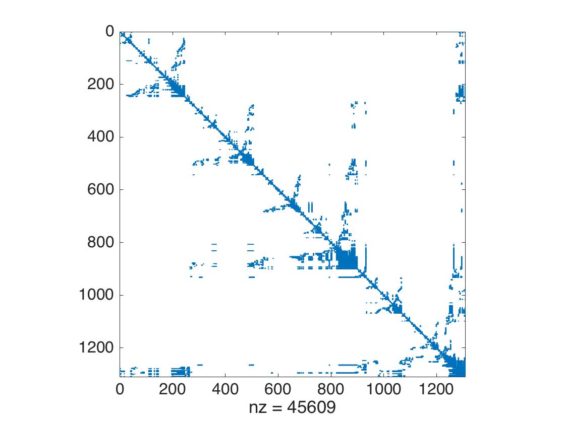 Figure 12
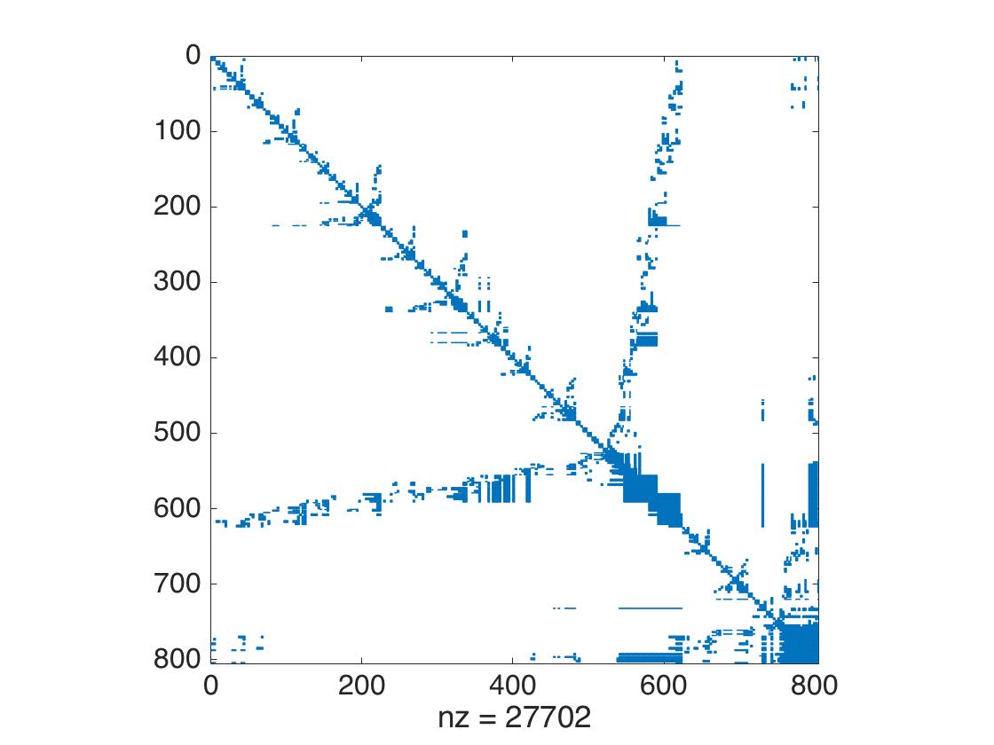 Figure 13
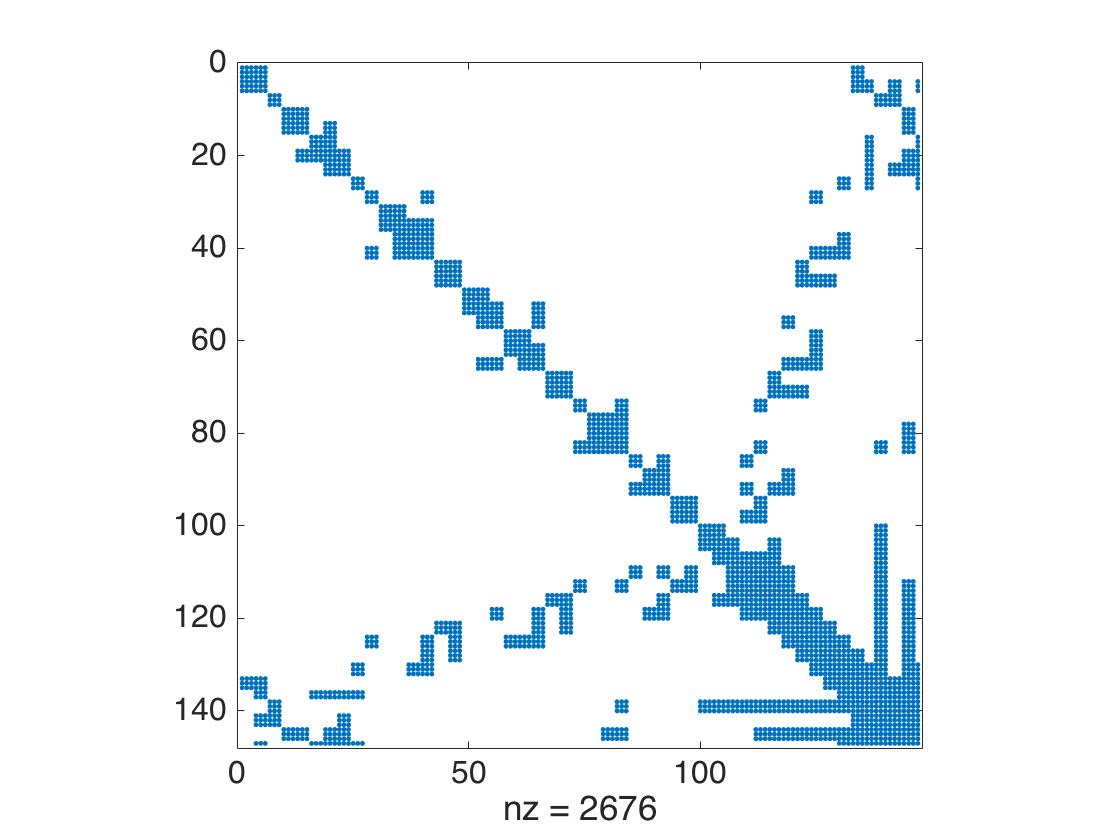 Figure 14
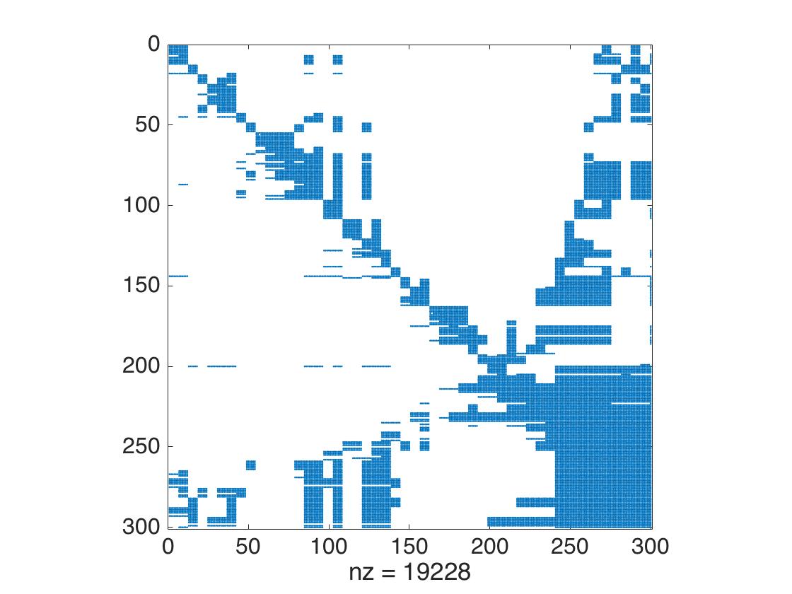 Figure 15
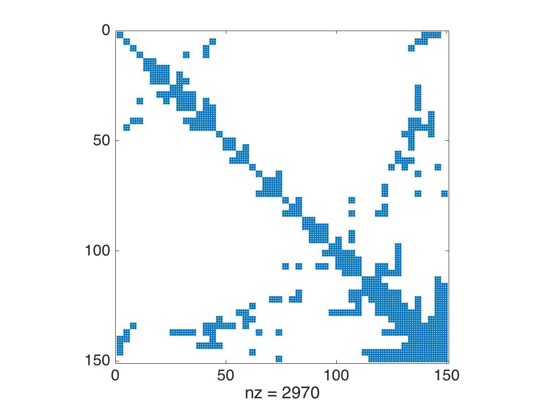 Figure 16
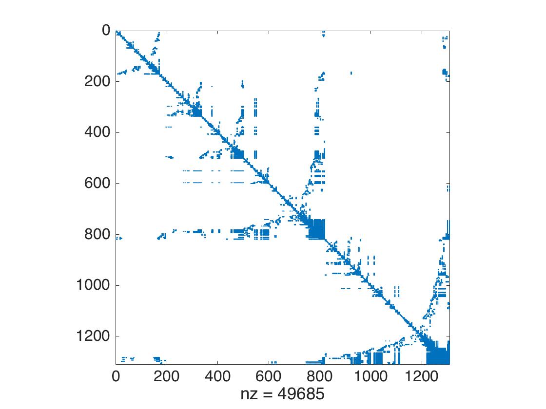 Figure 17
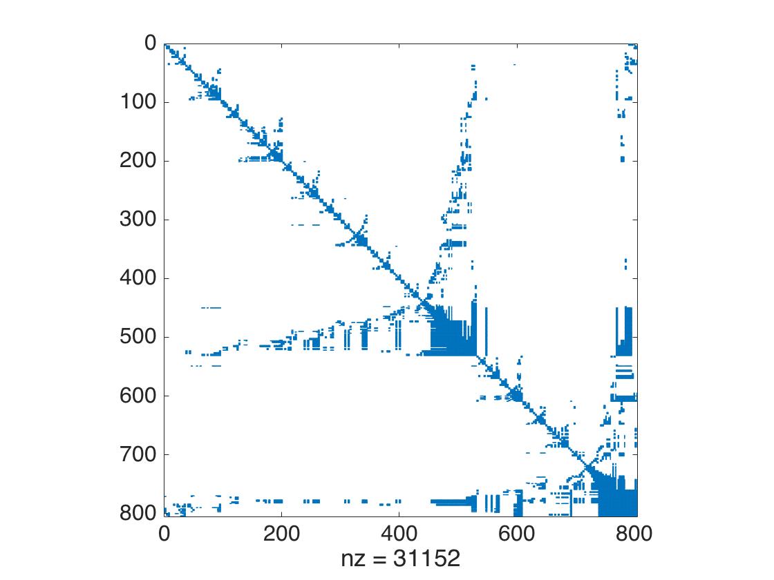 Figure 18
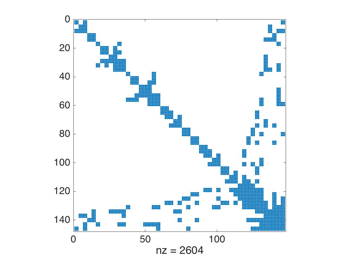 Figure 19
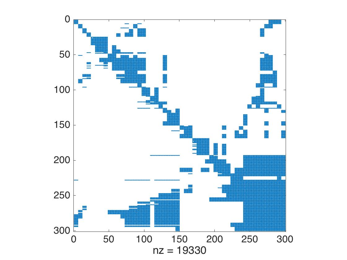 Figure 20
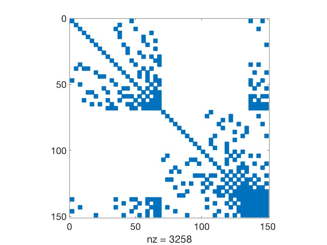 Figure 21
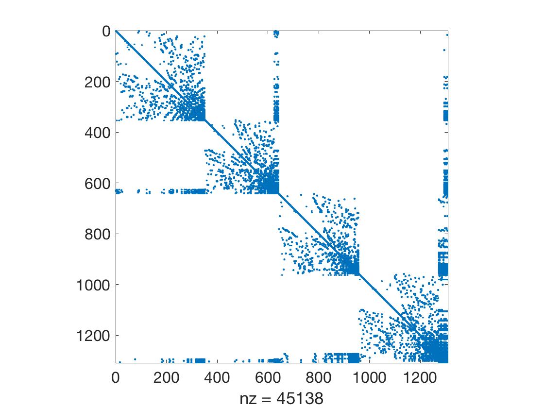 Figure 22
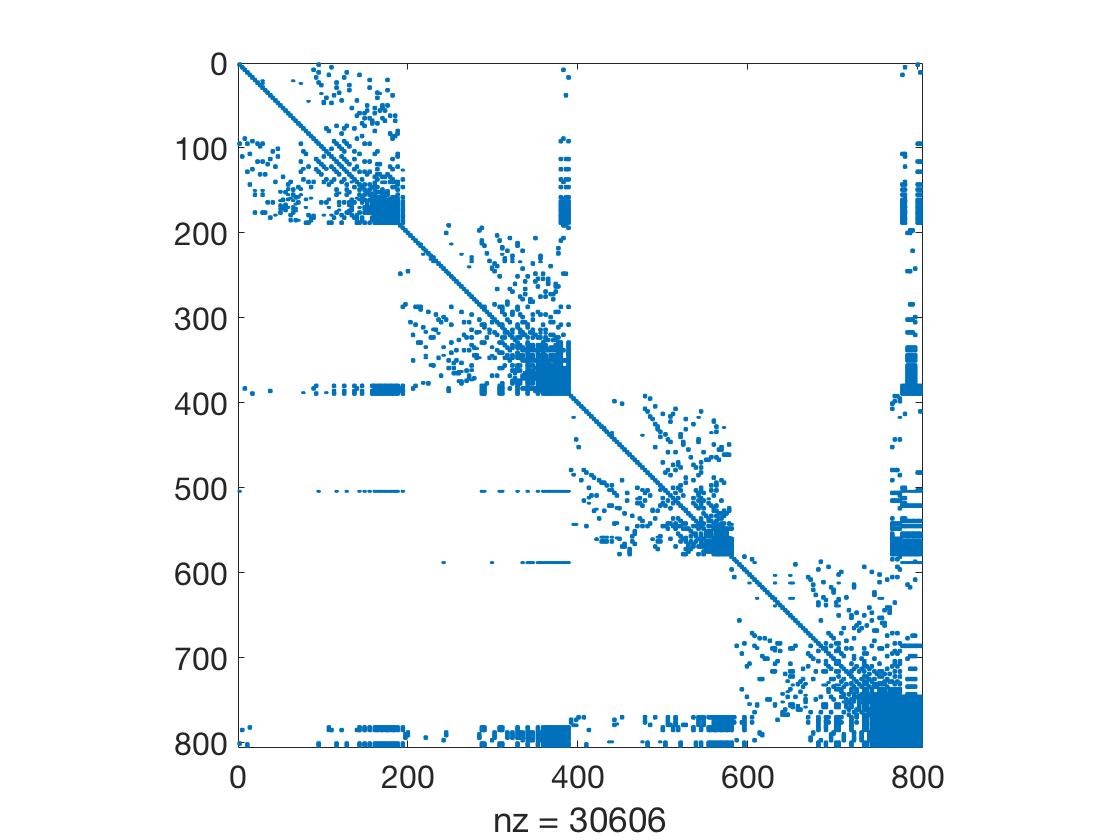 Figure 23
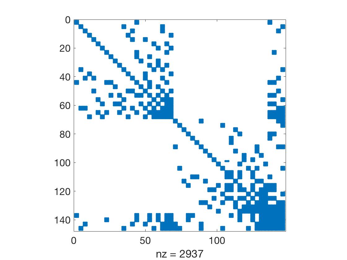 Figure 24
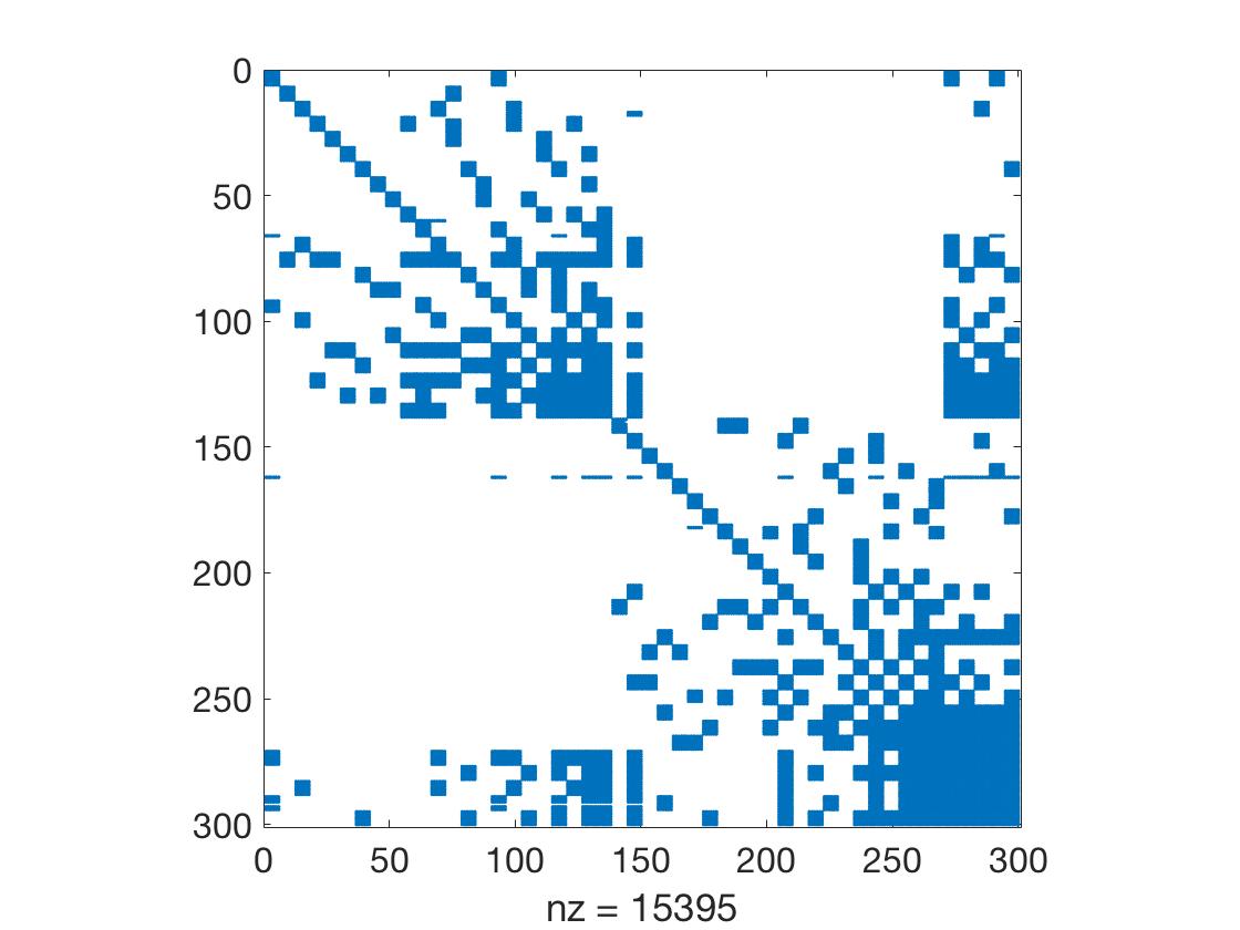 Figure 25
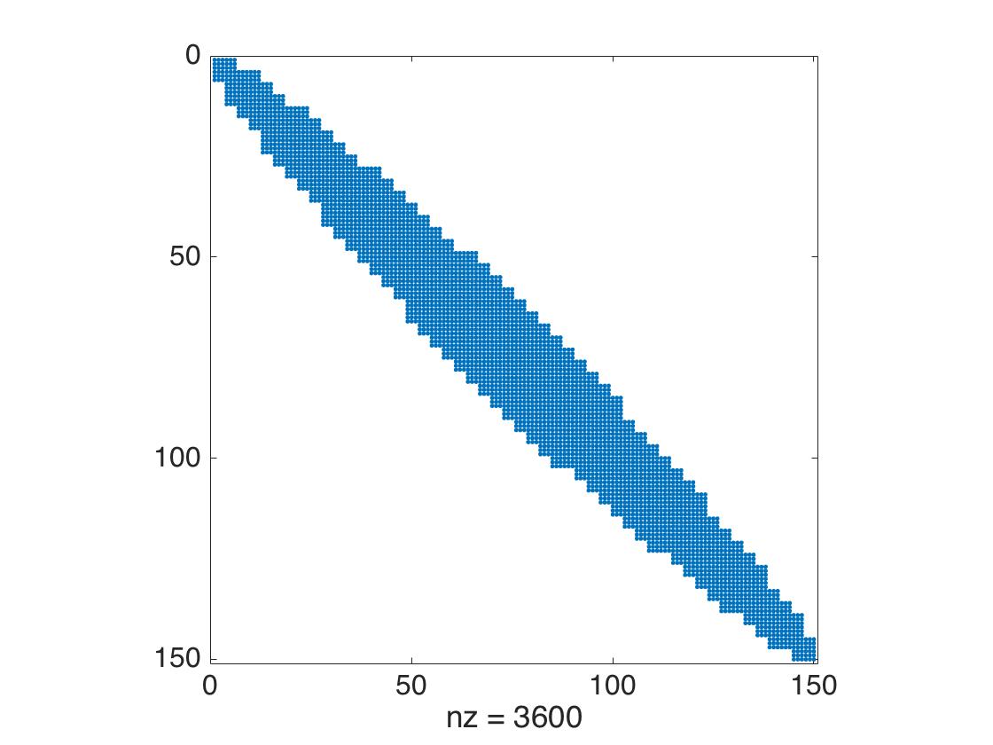 Figure 26
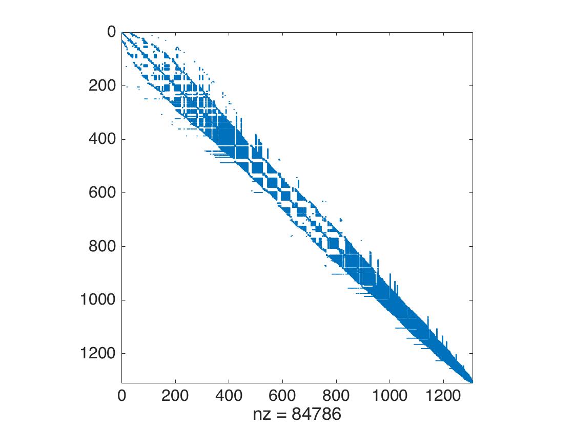 Figure 27
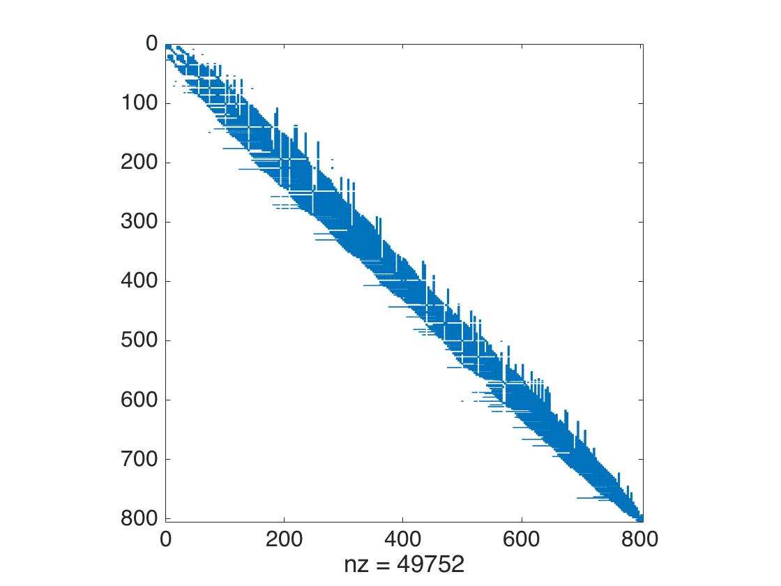 Figure 28
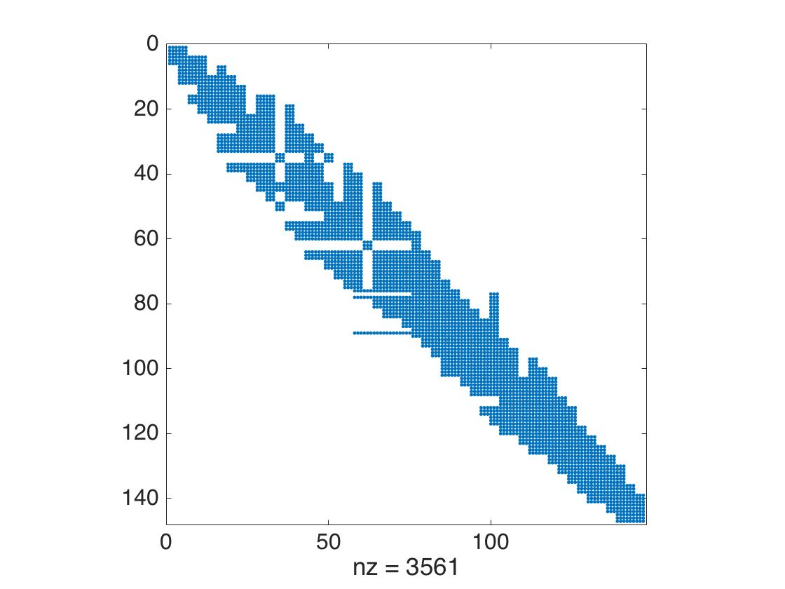 Figure 29
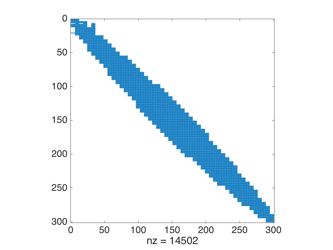 Figure 30
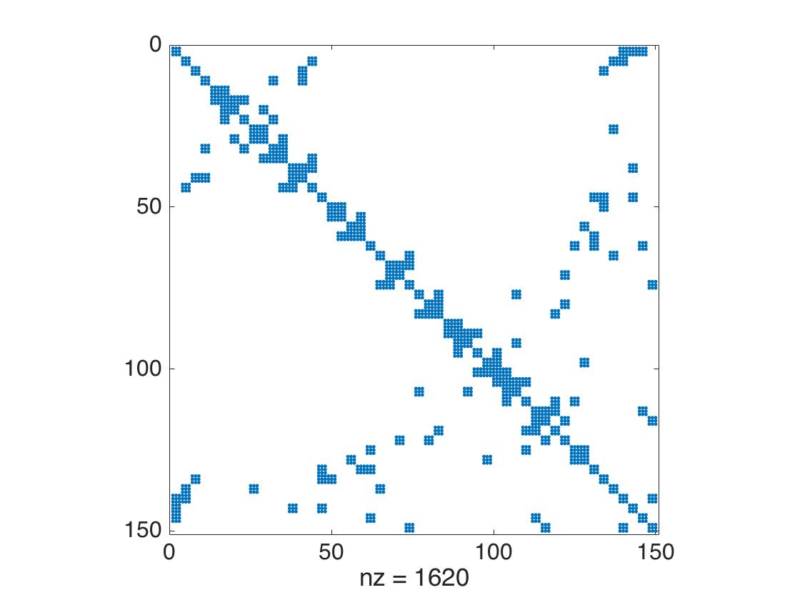 Figure 31
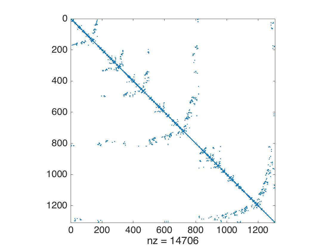 Figure 32
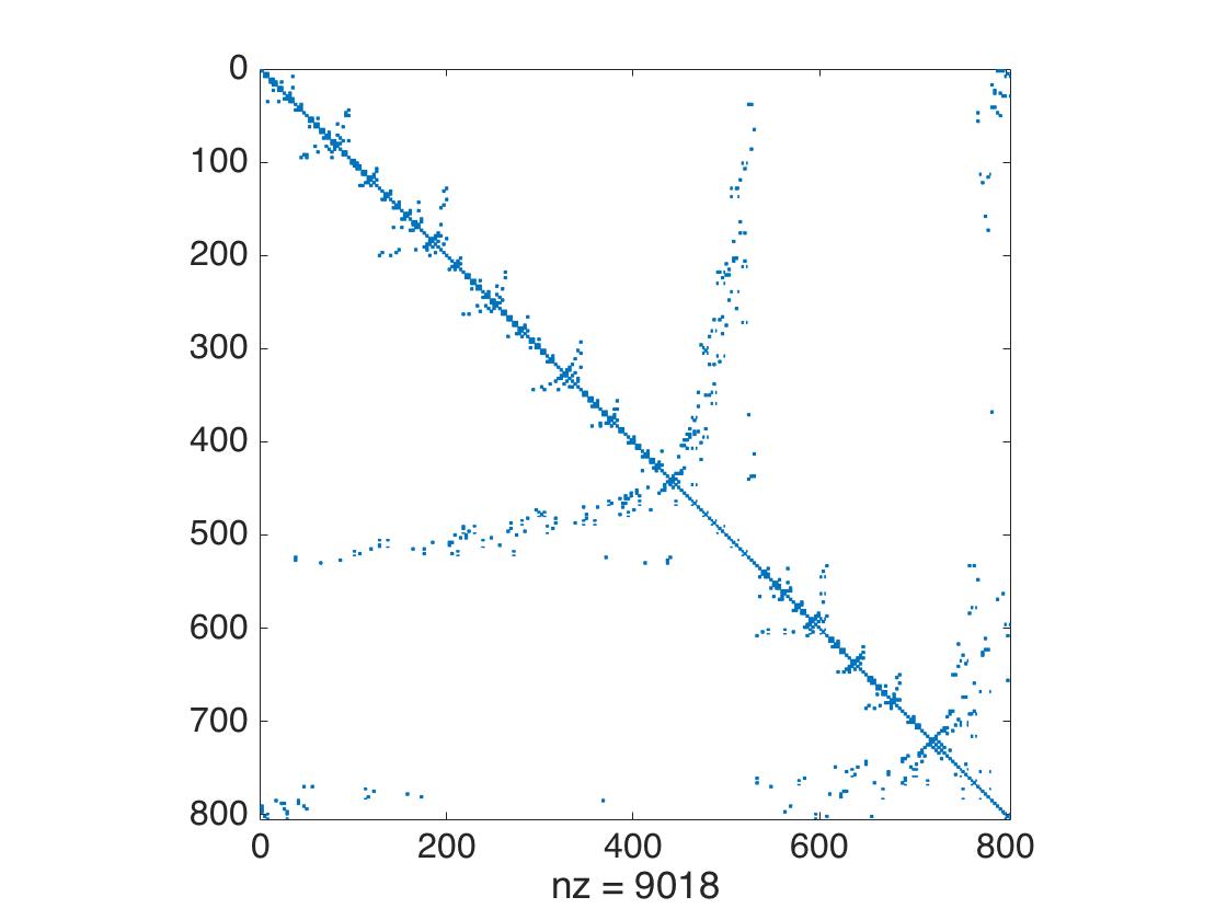 Figure 33
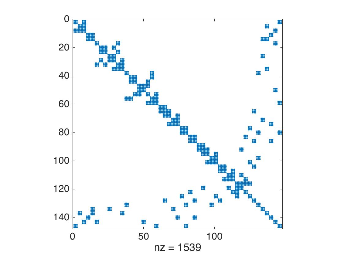 Figure 34
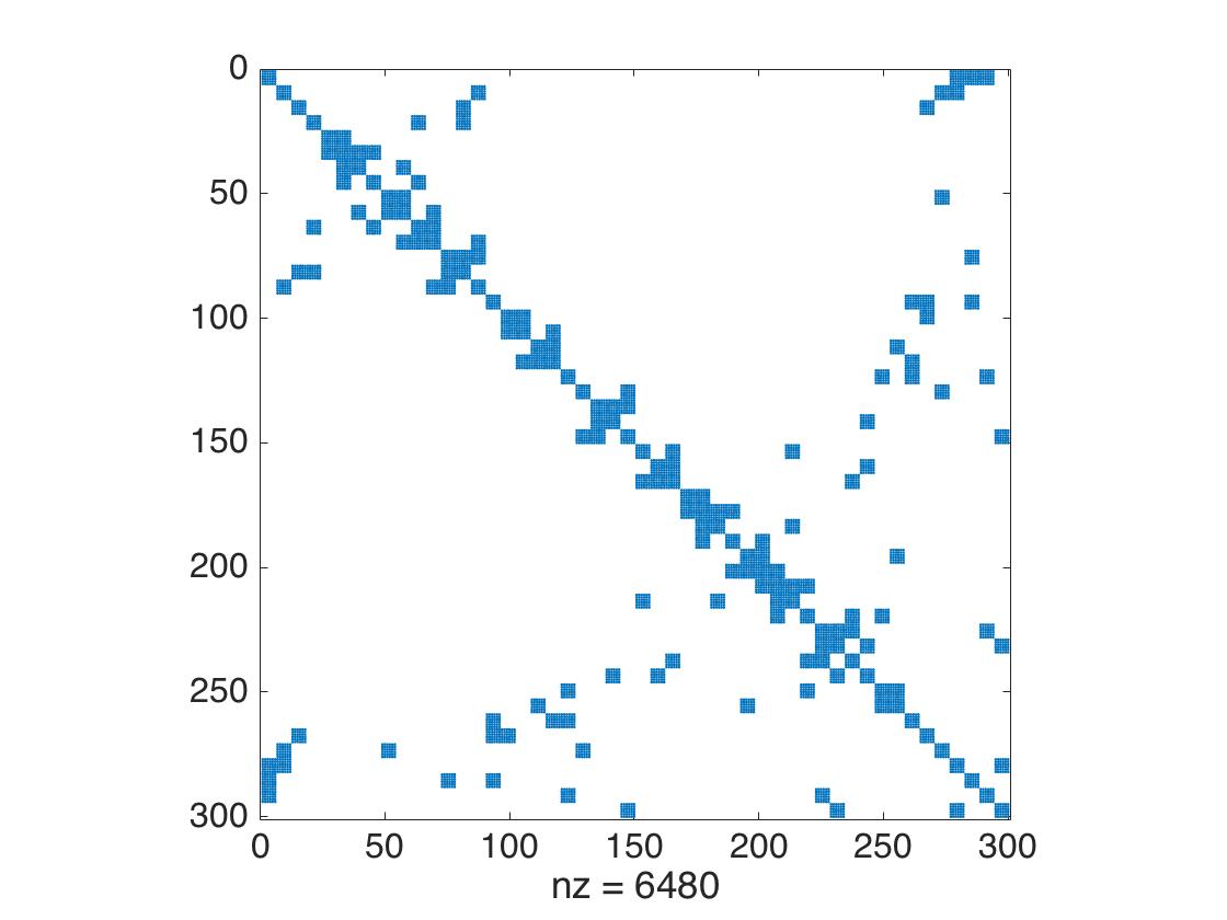 Figure 35
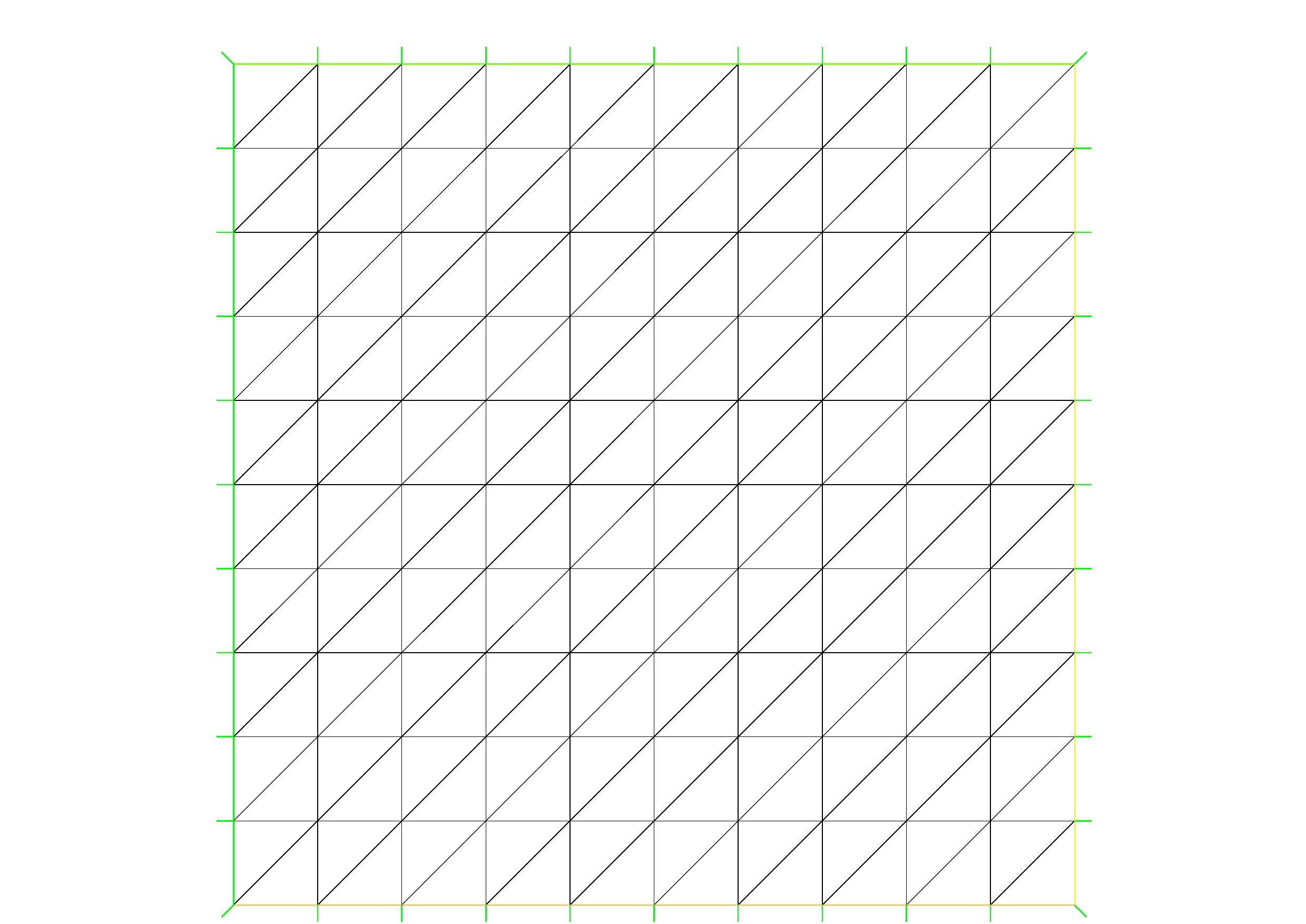 Figure 36
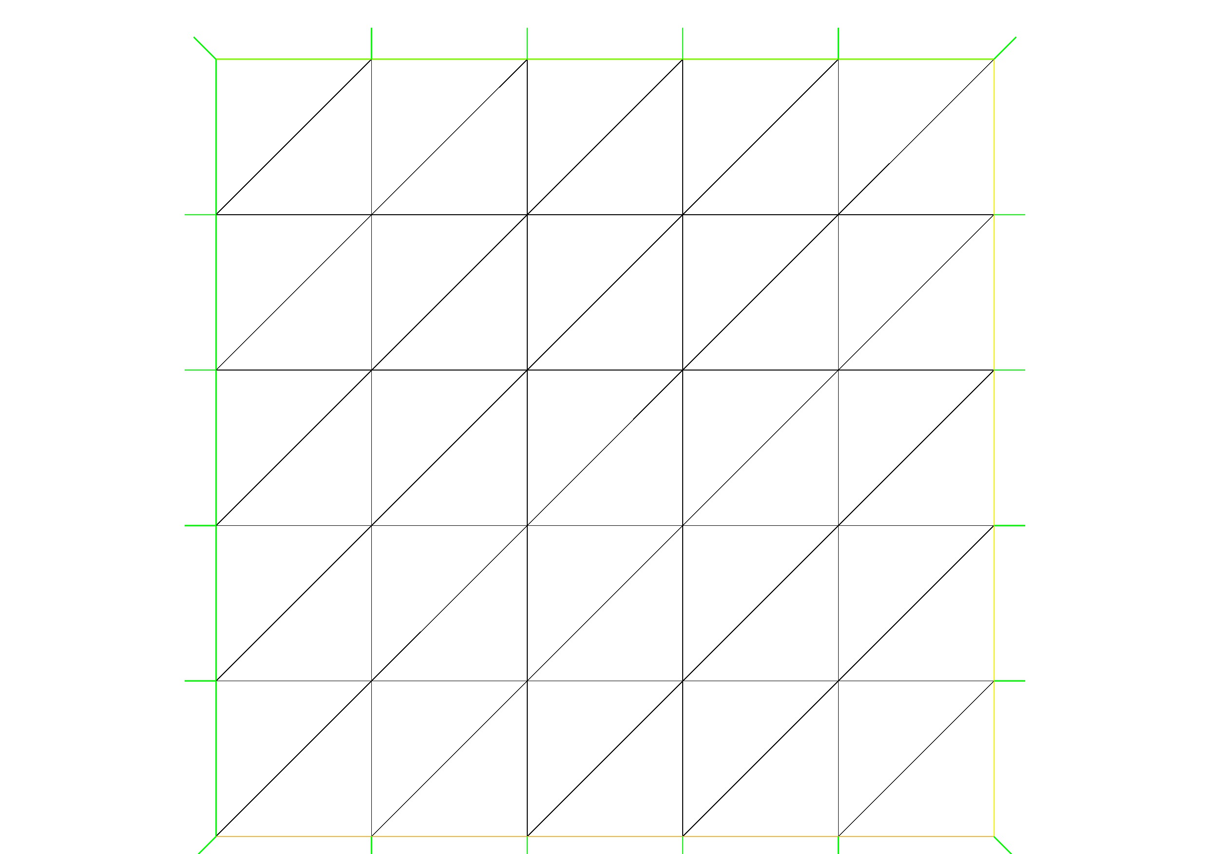 Figure 37
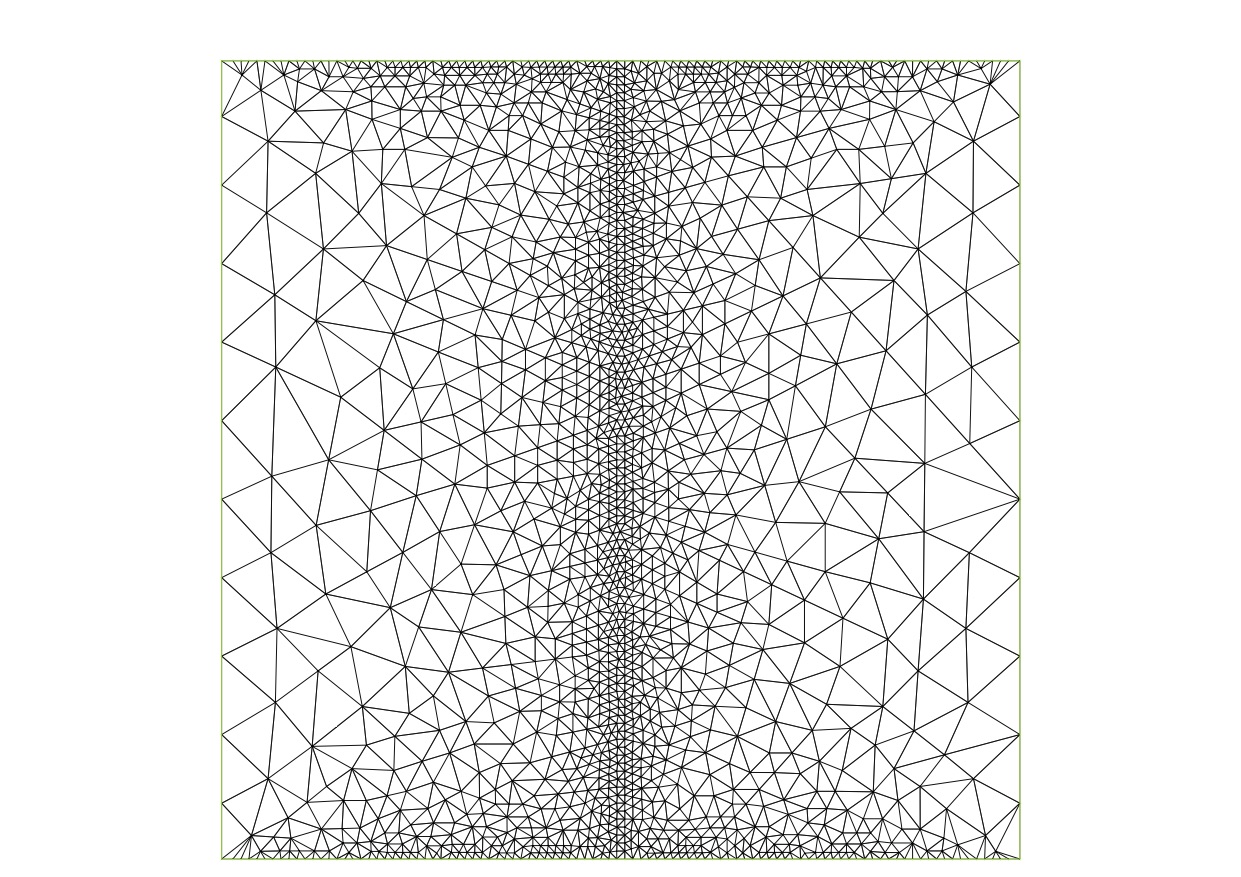 Figure 38
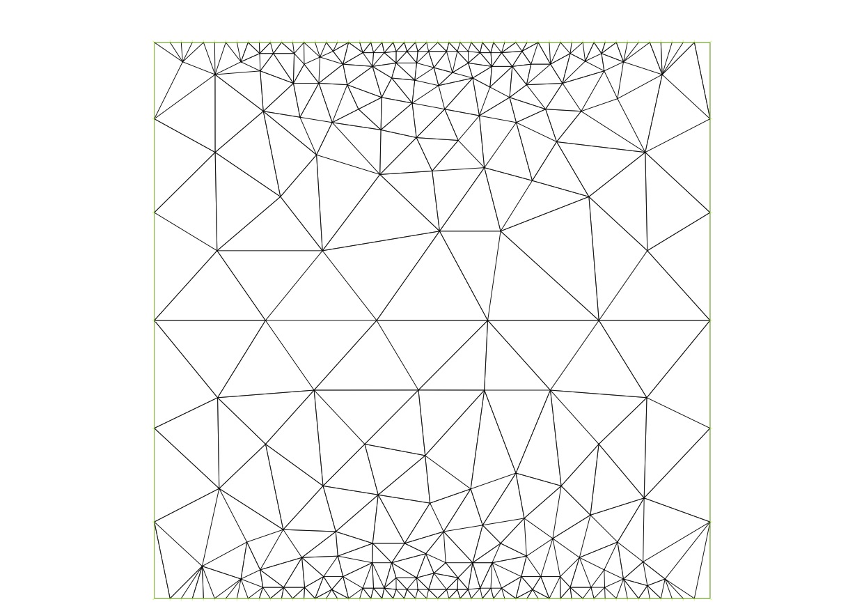 Figure 39
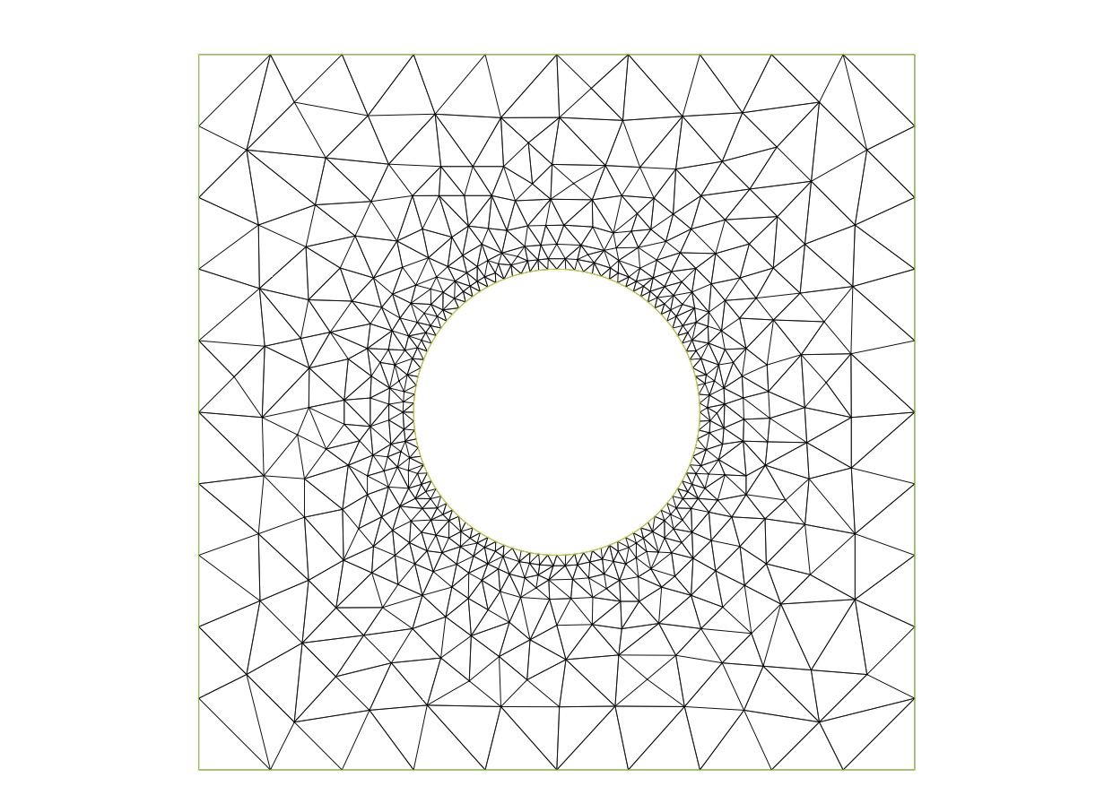 Figure 40
| n | Total Entries | Nonzero Entries | LU |
|---|---|---|---|
| 5 | 22500 | 1620 | 4680 |
| 10 | 6840 | 36810 | |
| 15 | 15660 | ||
| 20 | 28080 |
| n | Nonzero Entries | LU | AMD | ND | RCM |
|---|---|---|---|---|---|
| 5 | 7.2 % | 20.8 % | 13.2 % | 14.5 % | 16 % |
| 10 | 1.9 % | 10.2 % | 5.7 % | 5.7 % | 7.4 % |
| 15 | 0.86 % | 6.8 % | 3.8 % | 3.4 % | 4.8 % |
| 20 | 0.49 % | 5.1 % | 2.7 % | 2.3 % | 3.5 % |
| n | Total Entries | Nonzero Entries | LU |
|---|---|---|---|
| 5 | 14706 | 93387 | |
| 10 | |||
| 15 | |||
| 20 |
| n | Nonzero Entries | LU | AMD | ND | RCM |
|---|---|---|---|---|---|
| 5 | 0.86 % | 5.5 % | 2.7 % | 2.6 % | 4.96 % |
| 10 | 0.12 % | 4.6 % | 1.4 % | 0.98 % | 3.4 % |
| 15 | 0.11 % | 2.6 % | 1.2 % | 1.0 % | 2.2 % |
| 20 | 0.031 % | 4.02 % | 1.3 % | 0.75 % | 2.02 % |
| n | Total Entries | Nonzero Entries | LU |
|---|---|---|---|
| 5 | 21609 | 1539 | 4032 |
| 10 | 5670 | 24749 | |
| 15 | 12753 | ||
| 20 | 23076 |
| n | Nonzero Entries | LU | AMD | ND | RCM |
|---|---|---|---|---|---|
| 5 | 7.1 % | 18.7 % | 12.4 % | 13.6 % | 16.5 % |
| 10 | 2.2 % | 9.5 % | 6.8 % | 7.1 % | 8.3 % |
| 15 | 1.02 % | 9.4 % | 3.9 % | 3.8 % | 6.2 % |
| 20 | 0.58 % | 7.99 % | 3.2 % | 3.1 % | 4.8 % |
| n | Total Entries | Nonzero Entries | LU |
|---|---|---|---|
| 5 | 9018 | 49113 | |
| 10 | 33732 | ||
| 15 | 78174 | ||
| 20 |
| n | Nonzero Entries | LU | AMD | ND | RCM |
|---|---|---|---|---|---|
| 5 | 1.4 % | 7.6 % | 4.3 % | 4.7 % | 7.7 % |
| 10 | 0.4 % | 3.6 % | 2.3 % | 2.2 % | 4.03 % |
| 15 | 0.18 % | 2.4 % | 1.96 % | 1.3 % | 2.9 % |
| 20 | 0.098 % | 2.6 % | 1.96 % | 1.1 % | 2.3 % |
| n | Total Entries | Nonzero Entries | LU |
|---|---|---|---|
| 5 | 90000 | 6480 | 24275 |
| 10 | 27360 | ||
| 15 | 62640 | ||
| 20 |
| n | Nonzero Entries | LU | AMD | ND | RCM |
|---|---|---|---|---|---|
| 5 | 7.2 % | 26.97 % | 21.4 % | 17.1 % | 16.1 % |
| 10 | 1.9 % | 13.9 % | 22.7 % | 15.1 % | 8.1 % |
| 15 | 0.86 % | 9.7 % | 15.9 % | 12.8 % | 5.8 % |
| 20 | 0.49 % | 5.4 % | 13.1 % | 7.6 % | 4.3 % |
Peer Reviews
No public reviews on file for this paper yet. If you reviewed it on a platform where reviews are public (OpenReview, ICLR, NeurIPS, ICML), you can paste yours below so the community can read it here.
Videos
No videos yet. Explain this paper in a talk, walkthrough, or lecture? Add one.
Taxonomy
TopicsAdvanced Numerical Methods in Computational Mathematics · Numerical methods in engineering · Electromagnetic Simulation and Numerical Methods
An analysis of sparsity preserving pivot strategies for discontinuous Galerkin methods applied to acoustic scattering
Cody Lorton Department of Mathematics and Statistics, University of West Florida, Pensacola, FL 32514, U.S.A. ([email protected]).
Ryan Severance Department of Mathematics and Statistics, University of West Florida, Pensacola, FL 32514, U.S.A. ([email protected]).
Abstract
In this paper we discuss and analyze the sparse structure of matrices associated to the interior penalty discontinuous Galerkin (IP-DG) method applied to the Helmholtz equation. It is well-known that -factorization causes fill-in and this paper discusses three pivoting strategies: approximate minimal degree (AMD), nested dissection, and reverse Cuthill-McKee, that can reduce fill-in associated to the -factorization. Numerical experiments are included that demonstrate the performance of these pivoting strategies. These experiments include both uniform and non-uniform mesh structures, the inclusion of a scattering boundary, and both piecewise linear and quadratic solution spaces.
keywords:
Helmholtz equation, acoustic scattering, discontinuous Galerkin methods, sparse matrices, LU factorization, pivoting
1 Introduction
First, we will define the domain used to define the acoustic scattering model studied in this paper. Let and be two open and bounded sets in where is the spatial dimension for the problem. Further, assume that such that both and satisfy a star-shaped condition involving the same point. Define the domain with boundary . We will decompose the boundary into where and .
Using the domain defined above we define the following acoustic scattering model:
[TABLE]
(1) is the acoustic Helmholtz equation and is used to model time- harmonic acoustic waves in some homogeneous medium. In this equation models the displacement of the medium caused by the acoustic wave. The domain represents the acoustic medium in which the wave is traveling. is the wave number parameter of the wave and is defined as where is the angular frequency of the wave and is the speed of the wave. are given source functions.
In the boundary condition (2) refers to the unit outward normal vector to the domain and is the imaginary unit. Typically wave propagation models are posed on unbounded domains with far- field conditions dictating the behavior of the wave. These unbounded domains are computationally prohibitive. Thus, the above acoustic scattering model is defined on a bounded domain with boundary due to the truncation of an unbounded domain. To approximate an unbounded domain an absorbing boundary condition like (2) is used [14]. (2) simulates the absorption of the acoustic wave into the boundary .
The open and bounded set represents a scattering object in the homogeneous media. Thus, (3) is a scattering boundary condition. In particular, the homogeneous Dirichlet condition (3) used in this paper models a sound-soft scattering object.
This paper is mainly concerned with the case of a large wave number . It is well-known that in this case the Helmholtz differential operator is indefinite and this leads to difficulties in analyzing the Helmholtz PDE (1). Furthermore, numerical discretization techniques of the Helmholtz problem (1)–(3) lead to a non-Hermitian indefinite system of equations that must be solved to resolve the wave. This leads to subsequent difficulties in the numerical analysis of the discretization method as well as difficulties in solving the linear system.
Many discretization methods have been applied to the acoustic Helmholtz problem and analyzed. These include the finite element method (FEM) [3, 11, 12, 34, 37] , the plane wave discontinuous Galerkin (PW-DG) method [22, 24, 35], and the ultra weak variational form (UWVF) [5, 6, 7, 25, 26, 29]. It is well-known that one must use a fine enough spatial mesh when defining the discretization in order to resolve the wave length in each coordinate direction. This leads to a minimum mesh constraint of the form where is the mesh size parameter and represents the maximum diameter of each element of the partition of the spatial domain. In [27] the authors showed that this minimum constraint is necessary for the finite element method (FEM) applied to the 1-dimensional acoustic Helmholtz equation. Furthermore, in [27] it was shown that the error bound for the solution of the FEM applied to the 1-d acoustic Helmholtz equation contains a term of the order called the pollution term. This pollution term causes an increase in the error as is increased when is chosen to satisfy the minimum mesh constraint . The increase in error under the minimum mesh constraint is called the pollution effect. It has been shown that the pollution effect is inherent in Helmholtz-type problems and leads to a loss of stability in standard discretization techniques [4, 11]. Due to this loss of stability, a strict mesh constraint of the form (called the asymptotic mesh constraint) was required to obtain optimal and quasi-optimal error estimates for the acoustic Helmholtz problem [3, 11, 12].
In [17, 18] an interior penalty discontinuous Galerkin (IP-DG) method was developed and analyzed for the acoustic Helmholtz problem (1)–(3). This IP-DG method made use of purely imaginary penalty parameters and penalization of the jumps of function values, normal derivatives, and tangential derivatives. In [17, 18] this IP-DG method was shown to be unconditionally stable. In particular, stability estimates were obtained in both the asymptotic and pre-asymptotic mesh regime. Also, sub-optimal error estimates were proven in the pre-asymptotic mesh regime which improve to optimal order error estimates in the asymptotic mesh regime. Numerical experiments in [17] show that when is large the IP-DG method outperforms the standard FEM in the number of degrees of freedom required to attain a given accuracy. For these reasons, we will focus on this unconditionally stable IP- DG method in this paper.
To resolve the solution of the acoustic Helmholtz problem (1)–(3) with large using standard discretization techniques, one must solve a large non-Hermitian, indefinite, and ill-conditioned system of linear equations. In [15] it was shown that standard iterative solvers applied the the acoustic Helmholtz problem do not perform well. In fact, many do not converge. Thus, to resolve the solution of the acoustic Helmholtz problem a direct linear solver is usually employed. In [16] an direct solver was used to obtain an efficient and accurate discretization method for the acoustic Helmholtz problem in random media.
In this paper, we will study the decomposition of the system of equations obtained from the IP-DG method applied the the acoustic Helmholtz problem (1)–(3). The IP-DG method leads to a linear system defined with a sparse global matrix . It is well-known that the decomposition leads to “fill-in” of the sparse system and thus requires more CPU memory and leads to a loss of efficiency [20, 21]. To reduce fill-in, one can use pivoting prior to the decomposition. This paper will study three popular sparsity preserving pivoting strategies applied to the linear system obtained from the IP-DG method [17, 18]: (1) minimum degree pivoting, (2) nested dissection, and (3) bandwidth/profile reduction. We will use numerical experiments to compare the fill-in produced by the decomposition after using these pivoting strategies.
The paper is organized as follows. Section 2 will detail the IP- DG method used in this paper. Section 3 will discuss the sparse structure of the global matrix defined by the IP-DG method and detail the three sparsity preserving pivoting methods that we will study in this paper. Section 4 will be used to discuss multiple numerical experiments that were designed to study pivoting to preserve the sparsity of the global matrix obtained from the IP-DG method. Section 5 will be used to summarize the results and offer conclusions.
2 Interior penalty discontinuous Galerkin method for acoustic scattering
The goal of this section is to introduce the reader to the interior penalty discontinuous Galerkin (IP-DG) method developed and analyzed in [17, 18]. For more in-depth information regarding this discretization we encourage the reader to see those papers. In order to define the IP-DG method we will need to introduce standard notation used to define DG methods. For more understanding of discontinuous Galerkin (DG) methods we refer the reader to [36].
2.1 DG Notation
This subsection will be used to introduce the notation used to define the IP-DG method studied in this paper. Throughout this paper we will use the standard complex-valued -space norm and inner product notation. In particular, for and we let and denote the complex -inner product on and , respectively. That is,
[TABLE]
To discretize the PDE problem (1)–(3) using the discontinuous Galerkin method, let be a shape regular partition of the domain parameterized by the size parameter . Typically is a triangulation of a domain in and specifies the maximum diameter of a triangle . Example triangulations used in later numerical experiments are given throughout Section 4 (see Figures 1, 6,11, and 16).
One key characteristic of discontinuous Galerkin methods is the use of an energy space to derive the weak formulation. This function space includes functions that are discontinuous at edge/face boundaries of the partition . To deal with these discontinuities we will need to define special notation that is standard in discontinuous Galerkin method. We begin by defining the following sets of edges/faces:
[TABLE]
For any there exists two cells such that . For such an edge/face , let be the unit normal vector pointing out of if has larger global label and pointing out of if has larger global label. Also for an edge/face we define the jump and average operators of a function in the following way:
[TABLE]
For we define to be the unit outward normal vector on and . For , let be an independent set of unit tangential vectors to and .
To define the IP-DG method for (1)–(3), we define the finite dimensional solution space , where is a positive integer. In other words is the set of piecewise polynomials of degree over the partition . In numerical experiments later in this paper we will focus on the cases of , i.e. solutions that are piecewise linear or quadratic over the partition . Over the space we define the following sesquilinear form from [17, 18]:
[TABLE]
where
[TABLE]
The IP-DG method developed and analyzed in [17, 18] and used in this paper is defined as: Find such that
[TABLE]
The terms are referred to in the DG literature as penalty terms with called penalty parameters. This IP-DG method is characterized by penalization of jump discontinuities in the function values, normal derivatives, and tangential derivatives at cell boundaries in the partition . The penalty parameters can be complex values with positive real part, but it has been shown that the imaginary part of these parameters do not improve performance [17]. Thus, we will assume the penalty parameters are positive real numbers. With this in mind, the penalty terms in (6) characterize purely imaginary penalization which is a unique characteristic of this method.
The key feature of this method, is the unconditional stability of the method. In [17, 18], stability estimates were proven for any positive parameters . In contrast, for standard discretization methods such as the finite element method, stability estimates are only proven in the asymptotic mesh regime . The unconditional stability of the IP-DG method in (6) leads to unconditional unique solvability of the IP-DG problem . The IP-DG method is also proven to be optimally convergent in the asymptotic mesh regime and sub-optimally convergent in the preasymptotic mesh regime [17, 18].
3 Sparsity preserving pivot strategies
It is well-known that the IP-DG method (6) is equivalent to solving a system of linear equations of the form
[TABLE]
In this section, we will discuss the sparse properties of this linear system as well as sparsity preserving pivoting strategies that can be used to reduce fill-in of the decomposition.
First, we note that the IP-DG function space is a finite dimensional subspace of , thus there exists a basis of . Recall, that is the space of piecewise linear polynomials over the partition . A typical basis function used in IP-DG methods for takes the form
[TABLE]
where is a single cell in the partition . In other words, a typical basis function is a polynomial on a single cell that is 0 on all other cells of .
Given a basis of the linear system in (7) is defined by , where
[TABLE]
and the IP-DG solution is defined as
[TABLE]
Thus, for a basis comprised of functions with support on a single cell ,
[TABLE]
if and only if and are basis functions associated to the same cell or neighboring cells of the partition . Thus, the matrix is a sparse matrix. Also, since for real-valued basis functions in (5), then is symmetric. The distribution of nonzero element in depends on the enumeration of the partition as well as the basis functions used.
As stated earlier in the paper, we will focus on an factorization as the method for solving the system in (7). It is well known that the factorization causes fill-in of sparse systems. To mitigate this fill-in, we will use different permutation matrices such that the permuted matrix has an factorization with less fill-in. In this paper, will test three sparsity preserving pivoting strategies for the system (7). These are minimum degree pivoting (MDP), nested dissection (ND), and bandwidth/profile reducing pivoting. These methods were developed for the Cholesky factorization of a symmetric positive definite matrix, but can also be applied to the factorization of a more general square matrix. [10] discusses these pivoting strategies and others in depth.
MDP was developed as a sparsity preserving pivoting strategy in calculating a right-looking sparse Cholesky factorization. In particular, MDP is a greedy algorithm with the goal of choosing the sparsest pivot row and column in each step of the Cholesky factorization. MDP was first introduced by Markowitz in [30]. In this paper we use the approximate minimal degree (AMD) pivoting algorithm developed by Amestoy, Davis, and Duff [1, 2]. For numerical experiments discussed in Section 4 we made use of Matlab’s amd function [31] to obtain the AMD permutation matrix .
The nested dissection (ND) permutation was developed by George [19]. The ND permutation was designed specifically to reduce fill-in due to Cholesky factorization applied to linear systems generated by the finite element method. ND might be a good choice for the matrices discussed in this paper due to the similarities between the matrix generated by the finite element method and the IP-DG method. Duff, Erisman, and Reid [13] made an early comparison of MDP and ND permutations. For numerical experiments discussed in Section 4 we made use of Matlab’s dissect function [32] to obtain the ND permutation matrix .
The last class of pivoting strategies that we consider is one in which is generated such that the bandwidth/profile of is decreased, thus reduces the fill-in from the decomposition. One of the first pivoting techniques developed for bandwidth/profile reduction was developed by Cuthill and McKee in [9]. Later Liu and Sherman introduced the reverse Cuthill McKee (RCM) method [28]. RCM reverses the Cuthill-McKee ordering which can further reduce the profile of the matrix. Chan and George developed an efficient RCM algorithm in [8]. For numerical experiments discussed in Section 4 we made use of Matlab’s symrcm function [33] to obtain the RCM permutation matrix .
4 Numerical experiments
In this section, we present a number of numerical experiments with the intent to compare the performance of approximate minimal degree (AMD), nested dissection (ND), and reverse Cuthill-McKee (RCM) pivoting strategies. In particular, we will observe the percent of fill-in when an factorization is used without these pivoting strategies and after these pivoting strategies have been used. The results will be presented using tables that specify the total number of nonzero entries compared to the total number of entries, as well as a table that gives the percent of fill-in. In addition to these tables, plots will be used to demonstrate the sparsity structure of the matrix before and after pivoting as well as the decomposition before and after pivoting. These plots were generated using Matlab’s spy function. To save space, the plots of the factorization show the combined factorization defined as where is the identity matrix of the same size as and .
In all experiments in this section we let be the unit square at the origin and . Since our intent is only to study the matrix defined in (7) and its factorization it is unnecessary to specify the functions in (1) and (2). Since the structure of the matrix depends on the structure of the mesh and the function space used in the IP-DG method (6), our experiments are conducted on using different mesh structures and function spaces. Following [17], we chose the following mesh parameters for each experiment
[TABLE]
To produce the mesh and matrix associated to the IP-DG method, FreeFEM++ [23] was used. All matrix analysis was done using Matlab’s built-in functions. All experiments were conducted on the same Mac computer with a 2 GHz Intel Core i7 processor and 8 GB 1600 MHz DDR3 RAM.
4.1 Numerical experiment 1
In this first set of experiments the scattering portion of the domain was chosen to be . Thus, and . To define the mesh we used a uniform triangulation of with intervals along each side of . The mesh size parameter is then defined as . Examples of the mesh used in this experiment are displayed in Figure 1. In this set of experiments the IP-DG function space was used, i.e. the set of piecewise linear functions across the triangulation .
Figure 2 demonstrates the sparse structure of the matrix along with its combined decomposition for . At the bottom of each figure the number of nonzero entries is given as . This figure demonstrates the fill-in associated to the factorization. Figures 3–5 show the sparsity structure of the permutation produced along with the factorization after permutation using AMD, ND, and RCM, respectively. From these images it is clear that the pivoting strategies give different sparsity structure and varying results with respect to fill-in reduction. Recall that RCM is designed to the reduce bandwidth/profile of the matrix . We can see this bandwidth/ profile reduction clearly in Figure 5.
Tables 1 and 2 summarize the results of experiment 1. In particular, Table 1 gives the number of total entries of the matrix , the number of nonzero entries of , the number of nonzero entries in the factorization of , and the number of nonzero entries of factorization of after AMD, ND, and RCM pivoting. Table 2 presents the same data from Table 1 as percentage of fill-in. From Table 2 it is clear that factorization produces a large amount of fill-in. The percent of fill-in decreases as the mesh is refined. It is also clear that each pivoting strategy decreases the percent of fill-in which leads to improved performance. In this experiment both AMD and ND pivoting decreases fill-in better than RCM pivoting. For a coarse mesh AMD performs slightly better than ND, but as the mesh is refined ND performs slightly better than AMD. In fact, for a fine mesh using , ND reduced fill-in by a factor of 2.3. In contrast, for the same mesh, AMD reduces fill-in by a factor of 1.9 and RCM reduces fill-in by a factor of 1.5.
4.2 Numerical experiment 2
Similar to the experiments in Section 4.1, in this section we will let and use the IP-DG function space . The main difference between the experiments in this section and Section 4.1 is the use of a less structured triangular mesh . In this section we use a mesh defined using intervals along the vertical sides of and intervals along the horizontal sides of . Figure 6 shows examples of meshes used in this section. The structure of the mesh will determine the structure of the matrix in (4). Thus, we expect to see different results in this experiment. Similar to Section 4.1 the IP-DG function space was used in this set of experiments.
Similar to Section 4.1, we plotted the sparsity structure of the matrix and its combined factorization for . We also plotted the matrix after AMD, ND, and RCM pivoting along with the factorization of each of these pivoted matrices. These plots are given in Figure 7–10. Also, similar to Section 4.1 the data for the number of nonzero entries for the matrices in this set of experiments are summarized in Tables 3 and 4. From these tables we see that all three pivoting strategies reduce the fill-in associated to factorization in this set of experiments. Also, as the mesh parameter increases, the pivoting strategies perform better. In this experiment, RCM reduces fill-in the least and ND reduces fill-in the most. For instance, for , RCM reduces fill-in by a factor of and ND reduces fill-in by a factor of .
4.3 Numerical experiment 3
In the third set of numerical experiments presented in this paper, our goal was to observe the performance of sparsity preserving pivoting on a domain with a scattering boundary. With this goal in mind, a circular scattering domain
[TABLE]
was included. In this experiment we used a quasi-uniform triangular mesh generated by using intervals along each side of and along . Examples of the mesh generated by are given in Figure 11. Similar to Sections 4.1 and 4.2 the IP-DG function space was used in this set of experiments.
Figure 12 shows the sparsity structure of the matrix defined by (7) along with its combined factorization. Similarly, Figures 13–15 give the sparsity structure of after AMD, ND, and RCM pivoting along with the combined factorization of each matrix for . The number of nonzero entries for and the combined factorization of and after AMD, ND, and RCM are summarized in Table 5. Similarly, the percent of non-zero entries for the combined factorization of these matrices is given in Table 6.
The results of this experiment and summarized in Table 6 are similar to the results using the uniform mesh in Section 4.1. For instance, Table 6 indicates that AMD and ND reduce fill-in at roughly the same rate, with AMD performing slightly better for the coarse mesh and ND performing slightly better for the fine mesh . Similar to experiments in Section 4.1 and 4.2 all three pivoting strategies reduce fill-in associated to factorization and as increases the rate at which pivoting reduces fill-in increases. For the fine mesh given by , RCM reduces fill-in the least with a reduction factor of and ND reduces fill-in the most with a reduction factor of .
4.4 Numerical experiment 4
Similar to Section 4.3 this section studies the IP-DG method with a circular scattering domain define by (11). In this section we chose to use a non-uniform triangular mesh . The triangular mesh was generated using intervals along each side of and intervals along . Thus, is coarse along the boundary and fine along the boundary . Example meshes for are given in Figure 16. Similar to Sections 4.1–4.3 the IP-DG function space was used in this set of experiments.
The sparsity structure of the matrix defined in (7) along with its combined factorization are given in Figure 17. This is followed up with the sparsity structure of the pivoted matrix and the combined factorization of this matrix for the AMD, ND, and RCM pivot strategies in Figure 18–20. Tables 7 and 8 are used to summarize the data from the experiments in this section. In particular, Table 7 give the number of nonzero entries in the matrix , its factorization, and the factorization of the matrix after AMD, ND, and RCM pivoting has been applied. Table 8 presents this nonzero data as a percent of the total number of entries in the matrix.
In contrast to experiments in Sections 4.1–4.3, the RCM method does not perform well in the experiments in this section. In fact, RCM increases the fill-in for the cases of . RCM only reduces fill-in in the fine mesh case with , but even then the reduction is only by a factor of .
Similar to our previous experiments in Sections 4.1–4.3, the AMD method reduces fill- in at a greater rate than ND for a coarse mesh characterized by . As the mesh is refined ND reduces fill-in at a rate greater than AMD. For instance, when ND reduces fill-in at a rate of while AMD reduces fill-in at a rate of .
4.5 Numerical experiment 5
In the final set of experiments of this paper, we use the same domain and mesh as Section 4.1. See Figure 1 for examples of the computational mesh used in this experiment. In contrast to the experiments in Section 4.1, this section makes use of the finite dimensional function space in (6), i.e. the IP-DG method used in this section involves piecewise quadratic solutions across the triangulation . This change in the approximation space changes the structure of the global matrix in (7) and further leads to different results with regard to pivoting and fill-in.
Figure 21 shows the sparse structure of the matrix without pivoting and the sparse structure of the combined factorization of when . Figures 22–24 display the sparse structure of the pivoted matrix along with its combined factorization for the AMD, ND, and RCM pivoting strategies when . From these figures we see differences in the fill-in produced in this section compared to those in Section 4.1. In particular, we see that the amount of fill-in from factorization increased in this set of experiments. Tables 9 and 10 summarize the results of the experiments using intervals along each side of the domain to generate the mesh .
Surprisingly, unlike previous experiments the RCM method out-performs both AMD and ND for all experiments in this section. For a coarse mesh characterized by all three methods reduce fill-in with a reduction rate of by AMD, by ND, and by RCM. The performance of AMD and ND deteriorates as the mesh is refined in this set of experiments. In fact, fill-in increases in the cases of when using AMD and ND pivoting prior to the factorization. RCM continues to reduce fill-in when the mesh is refined, but for the rate of reduction is decreased to .
5 Conclusions
The results discussed in Section 4 demonstrate that pivoting strategies are effective in reducing the fill-in due to LU factorization applied to the coefficient matrix generated by the IP-DG method applied to the Helmholtz problem (1)–(3). For experiments using a piecewise linear solution space , AMD and ND reduced fill-in by similar amounts with AMD usually performing better than ND for coarse meshes and ND usually performing better than AMD for fine meshes (c.f. Sections 4.1, 4.3, and 4.4). In Section 4.2 ND performs better than AMD in both coarse and fine meshes. For a piecewise linear solution space we observe that RCM does reduce fill-in, but not by as large of a factor as AMD and ND (c.f. Sections 4.1–4.4). Surprisingly, for a piecewise quadratic solution space , RCM reduces fill-in by a larger factor than AMD and ND. In fact, Section 4.5 demonstrates that AMD and ND increase fill-in for the solution space when using a fine mesh.
The reference list from the paper itself. Each links out to its DOI / PubMed record.
- 1[1] P.R. Amestoy, T.A. Davis, and I.S. Duff. An approximate minimum degree ordering algorithm. SIAM J. Matrix Anal. Appl. , 17:886 – 905, 1996.
- 2[2] P.R. Amestoy, T.A. Davis, and I.S. Duff. Amd, an approximate minimum degree ordering algorithm. ACM Trans. Math. Software , 30:381 – 388, 2004.
- 3[3] A.K. Aziz and R. B. Kellogg. A scattering problem for the Helmholtz equation. In Advances in Computer Methods for Partial Differential Equations - III; Proceedings of the Third International Symposium, Bethlem, PA, June 20 - 22, 1979 , pages 93 – 95, New Brunswick, NJ, 1979. IMACS.
- 4[4] I.M. Babuška and S.A. Sauter. Is the pollution effect of the FEM avoidable for the Helmholtz equation considering high wave numbers? SIAM J. Numer. Anal. , 34(6):2392 – 2423, 1997.
- 5[5] A. Buffa and P. Monk. Error estimates for the ultra weak variational formulation of the Helmholtz equation. M 2AN , 42(6):925 – 940, 2008.
- 6[6] O. Cessenat and B. Després. Application of the ultra weak variational formulation to the two dimensional Helmholtz problem. SIAM J. Numer. Anal. , 35:255 – 299, 1998.
- 7[7] O. Cessenat and B. Després. Using plane waves as base functions for solving time harmonic equations with the ultra weak variational formulation. J. Comput. Acoust. , 11:227–238, 2003.
- 8[8] W.M. Chan and A. George. A linear time implementation of the reverse cuthill-mckee algorithm. BIT , 20:8 – 14, 1980.