Local metrics of the Gaussian free field
Ewain Gwynne, Jason Miller

TL;DR
This paper introduces the concept of local metrics for the Gaussian free field, establishing criteria for their equivalence and uniqueness, which underpin the mathematical foundation of Liouville quantum gravity.
Contribution
It defines local metrics for the GFF, provides criteria for their equivalence and determination by the field, forming a basis for LQG metric studies.
Findings
Criteria for bi-Lipschitz equivalence of local metrics
Conditions for a local metric to be determined by the GFF
Framework supporting the existence and uniqueness of LQG metrics
Abstract
We introduce the concept of a local metric of the Gaussian free field (GFF) , which is a random metric coupled with in such a way that it depends locally on in a certain sense. This definition is a metric analog of the concept of a local set for . We establish general criteria for two local metrics of the same GFF to be bi-Lipschitz equivalent to each other and for a local metric to be a.s. determined by . Our results are used in subsequent works which prove the existence, uniqueness, and basic properties of the -Liouville quantum gravity (LQG) metric for all , but no knowledge of LQG is needed to understand this paper.
Click any figure to enlarge with its caption.
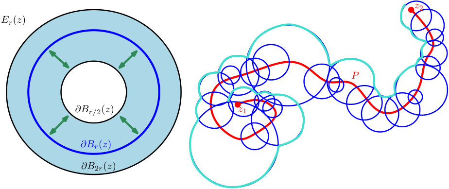 Figure 1
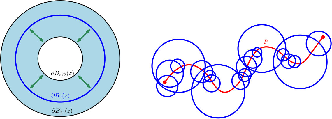 Figure 2
Peer Reviews
No public reviews on file for this paper yet. If you reviewed it on a platform where reviews are public (OpenReview, ICLR, NeurIPS, ICML), you can paste yours below so the community can read it here.
Videos
No videos yet. Explain this paper in a talk, walkthrough, or lecture? Add one.
Local metrics of the Gaussian free field
Ewain Gwynne and Jason Miller
Ewain Gwynne and Jason Miller
University of Cambridge
Abstract
We introduce the concept of a local metric of the Gaussian free field (GFF) , which is a random metric coupled with in such a way that it depends locally on in a certain sense. This definition is a metric analog of the concept of a local set for . We establish general criteria for two local metrics of the same GFF to be bi-Lipschitz equivalent to each other and for a local metric to be a.s. determined by . Our results are used in subsequent works which prove the existence, uniqueness, and basic properties of the -Liouville quantum gravity (LQG) metric for all , but no knowledge of LQG is needed to understand this paper.
Contents
1 Introduction
1.1 Overview
Let be an open planar domain. The Gaussian free field (GFF) on is a random distribution (generalized function) on which can be thought of as a generalization of Brownian motion but with two time variables instead of one, in the sense that the one-dimensional Gaussian free field is simply the Brownian bridge. We refer to Section 2.2, [She07], and/or the introductory sections of [SS13, She16, MS16c, MS17] for more on the GFF.
If is a coupling of with a random compact subset of , we say that is a local set for if for any open set , the event is conditionally independent from given .111The restriction of to an open set can be defined as the restriction of the distributional pairing to test functions which are supported on . The -algebra generated by for a closed set can be defined as , where is the Euclidean -neighborhood of . Hence it makes sense to speak of “conditioning on ” or to say that a random variable is “determined by ”. In other words, depends “locally” on , although is not required to be determined by . Local sets of were first defined in [SS13, Lemma 3.9]. Important examples of local sets include sets which are independent from as well as so-called “level lines” [SS13] and “flow lines” [MS16c, MS16d, MS16e, MS17] of , both of which are SLEκ-type curves that are a.s. determined by .
In this paper, we will study random metrics coupled with the GFF instead of random sets. As we will explain in more detail Section 1.3, this work is motivated by the question of constructing the Liouville quantum gravity metric for . This is the distance function associated with the Riemannian metric tensor “”, where denotes the Euclidean metric tensor on , which is in some sense a canonical model of a random two-dimensional Riemannian metric tensor. However, the ideas we develop here will apply in a more general framework.
We will now introduce a concept of a local metric of the GFF, which is directly analogous to the above definition of a local set. We first need some preliminary definitions. Suppose is a metric space.
For a curve , the -length of is defined by
[TABLE]
where the supremum is over all partitions of . Note that the -length of a curve may be infinite.
For , the internal metric of on is defined by
[TABLE]
where the infimum is over all paths in from to . Then is a metric on , except that it is allowed to take infinite values.
We say that is a length space if for each and each , there exists a curve of -length at most from to .
A continuous metric on an open domain is a metric on which induces the Euclidean topology on , i.e., the identity map is a homeomorphism. We equip the space of continuous metrics on with the local uniform topology for functions from to and the associated Borel -algebra. Note that the space of continuous metrics is not complete w.r.t. this topology. We allow a continuous metric to satisfy if and are in different connected components of . In this case, in order to have w.r.t. the local uniform topology we require that for large enough , if and only if .
Lemma 1.1**.**
Let be a continuous length metric on and let be open. The internal metric is a continuous length metric on .
Proof.
Since , it is clear that the identity map is continuous. To check that the inverse map is continuous, suppose is a sequence in which converges to with respect to the Euclidean topology. By the continuity of , for large enough , the -distance from to is smaller than the -distance from to . This implies that a path of near-minimal -length from to must stay in , so since is a length metric we have for large enough . By the continuity of , we have so also . ∎
Definition 1.2** (Local metric).**
Let be a connected open set and let be a coupling of a GFF on and a random continuous length metric on . We say that is a local metric for if for any open set , the internal metric is conditionally independent from the pair given .
By convention, we define to be a graveyard point in the probability space if . We emphasize that in Definition 1.2, is required to be conditionally independent from the pair given . This means that, unlike in the case of a local set, a random metric which is independent from is not necessarily a local metric for . If is determined by , then is a local metric for if and only if is determined by for each open set . If is not necessarily determined by , then Definition 1.3 implies that is conditionally independent from given ; see also Lemma 2.4 for a stronger version of this statement. See Section 2.3 for some equivalent formulations of Definition 1.2.
The goal of this paper is to prove several general theorems about local metrics of the GFF. We will give a condition under which two local metrics are bi-Lipschitz equivalent to each other (Theorem 1.6) and a condition under which a local metric is a measurable function of the field (Theorem 1.7).
As mentioned above, our results play an important role in related works [DDDF19, DFG*+*19, GM19a, GM19c, GM19b] which construct a certain special family of local metrics of the GFF: the -Liouville quantum gravity (LQG) metric for . We discuss these works further in Section 1.3. However, we emphasize that one does not need to know anything about LQG to understand this paper.
Acknowledgments. We thank an anonymous referee for helpful comments on an earlier version of this article. We thank Jian Ding, Julien Dubédat, Alex Dunlap, Hugo Falconet, Josh Pfeffer, Scott Sheffield, and Xin Sun for helpful discussions. EG was supported by a Herchel Smith fellowship and a Trinity College junior research fellowship. JM was supported by ERC Starting Grant 804166.
1.2 Main results
Before stating our main results concerning local metrics, we need some additional definitions which build on Definition 1.2.
Definition 1.3** (Jointly local metrics).**
Let be a connected open set and let be a coupling of a GFF on and random continuous length metrics. We say that are jointly local metrics for if for any open set , the collection of internal metrics is conditionally independent from given .
The following lemma gives a convenient way to produce jointly local metrics. See [SS13, Lemma 3.10] for the analog of the lemma for local sets.
Lemma 1.4**.**
Let be a coupling of a GFF on a domain with random continuous length metrics such that each for is local for and are conditionally independent given . Then are jointly local for .
Proof.
Fix . We first treat the case when . We will apply the following elementary probability fact: if is a coupling of three random variables such that is independent from , is independent from , and are conditionally independent given , then is independent from . See, e.g., [SS13, Lemma 3.5]. For our purposes, we will take
[TABLE]
and apply the statement to the conditional law of given .
Since and are conditionally independent given , the conditional law of given \mathopen{}\mathclose{{}\left(D_{1}(\cdot,\cdot;U\setminus\overline{V}),D_{2}(\cdot,\cdot;U\setminus\overline{V}),h}\right) is the same as the conditional law of given only \mathopen{}\mathclose{{}\left(D_{1}(\cdot,\cdot;U\setminus\overline{V}),h}\right). By the locality of , this is the same as the conditional law of given only . Hence, in the notation above, and are conditionally independent given . Similarly, and are conditionally independent given . Since and are conditionally independent given , it follows that also and are conditionally independent given and . The above probability fact therefore shows that is conditionally independent from given . This means precisely that and are jointly local for .
This completes the proof when . The case when follows from induction and a similar argument to the one above. ∎
We will sometimes work with GFF’s which are naturally defined modulo additive constant. When we do so, we will typically normalize the field so that its circle average over is zero for some and (see [DS11, Section 3.1] for the definition and basic properties of circle averages). We will be interested in local metrics which behave nicely when we make a different choice of normalization.
Definition 1.5** (Additive local metrics).**
Let be a connected open set and let be a coupling of a GFF on and random continuous length metric which are jointly local for . For , we say that are -additive for if for each and each such that , the metrics are jointly local metrics for .
The first main result of this article is the following criterion for two local metrics to be bi-Lipschitz equivalent. Roughly speaking, it states that if we can compare the distance across an annulus for one metric to the diameter of a circle w.r.t. the internal metric on an annulus for the other metric with high probability at all scales, then we get an a.s. global comparison of the metrics.
Theorem 1.6** (Bi-Lipschitz equivalence of local metrics).**
Let , let be a whole-plane GFF normalized so that , let , and let be a coupling of with two random continuous metrics on which are jointly local and -additive for . There is a universal constant such that the following is true. Suppose there is a deterministic constant such that for each compact set , there exists such that
[TABLE]
Then a.s. for each .
We also have a criterion for a local metric to be determined by , which says that, roughly speaking, if a local metric is determined by up to bi-Lipschitz equivalence then it is in fact itself determined by .
Theorem 1.7** (Measurability of local metrics).**
Let , let be a GFF on , and let be a coupling of with a random continuous length metric which is local for . Assume that is determined by up to bi-Lipschitz equivalence in the following sense. Suppose we condition on and let be conditionally i.i.d. samples from the conditional law of given . There is a random constant , depending only , such that a.s. for each . Then is a.s. determined by , i.e., one can take .
Combining Theorem 1.6 with Theorem 1.7 yields the following corollary.
Corollary 1.8**.**
There is a universal constant such that the following is true. Let be a domain which contains the unit disk, let be a whole-plane GFF normalized so that , and let be a coupling of with a random continuous length metric on which is local for and satisfies the following hypotheses.
* is -additive for for some (Definition 1.5).* 2. 2.
Condition on and let and be conditionally i.i.d. samples from the conditional law of given . There is a deterministic constant such that for each compact set , there exists such that (1.3) holds for this choice of and .
Then is a.s. determined by .
Proof.
We first claim that is a pair of -additive local metrics for . We know from Definition 1.5 that for each and each such that , each of and is individually local for . Since , it follows that and determine each other. Since and are conditionally independent given , they are also conditionally independent given . By Lemma 1.4, these two metrics are jointly local for . Theorem 1.6 tells us that if (1.3) holds for a large enough universal , then a.s. for each . Therefore, Theorem 1.7 implies that is a.s. determined by . ∎
1.3 Applications to Liouville quantum gravity
Here we briefly summarize how our results are used in the construction of the -Liouville quantum gravity (LQG) metric for general . This section is included only for context and is not needed to understand the rest of the paper.
For , a -LQG surface is, heuristically speaking, the random two-dimensional Riemannian manifold parameterized by a domain whose Riemannian metric tensor is , where is some variant of the GFF on and is the Euclidean metric tensor. This definition does not make literal sense since the GFF is only a distribution, not a function, so cannot be exponentiated. So, one needs to use regularization procedures to define LQG rigorously. Previous work has constructed the volume form associated with an LQG surface, called the -LQG area measure [Kah85, DS11, RV14]. This is a random measure which can be obtained as a limit of regularized versions of , where denotes Lebesgue measure.
It is expected that a -LQG surface also admits a canonical metric. This metric should be a local metric for which is, in some sense, obtained by exponentiating . Previously, such a metric was only constructed in the special case when [MS15, MS16a, MS16b], in which case the associated metric space is isometric to the Brownian map [Le 13, Mie13].
Ding, Dubédat, Dunlap, and Falconet [DDDF19] showed that for general , a certain natural approximation scheme for the -LQG metric called Liouville first passage percolation (LFPP) admits non-trivial subsequential limiting metrics. To construct a metric on -LQG, one wants to show that there is a unique subsequential limit and that it satisfies certain scale invariance properties. This is accomplished in [GM19c], building on [DFG*+*19, GM19a] and the present paper.
It can be checked that every subsequential limit of LFPP is a local metric of the GFF (see [DFG*+*19, Section 2]). Hence our results can be applied to study such subsequential limits. In particular, Corollary 1.8 will be used in [DFG*+*19] to show that every subsequential limit can be realized as a measurable function of the GFF. Theorem 1.6 is used in [GM19c] to show that certain pairs of subsequential limiting metrics are bi-Lipschitz equivalent, which reduces the problem of proving uniqueness of the subsequential limit to the (quite involved) problem of showing that the two bi-Lipschitz equivalent metrics in fact differ by a scaling (i.e., the ratio of the two metrics is a positive and finite constant). Theorem 1.6 is also used in [GM19b] as an intermediate step in the proof of the conformal covariance of the LQG metric.
1.4 Outline
The rest of this paper is structured as follows. In Section 2.2, we review some facts about the Gaussian free field and record some elementary properties of local metrics. In Section 3 we prove a general lemma (Lemma 3.1) concerning the near-independence of events which depend on the GFF and a collection of jointly local metrics restricted to disjoint concentric annuli. This lemma is an extension of a result from [MQ18] and will also be used in [DFG*+*19, GM19a, GM19c, GM19b]. In Section 4, we use this general “independence across annuli” lemma to prove Theorem 1.6. In Section 5, we prove Theorem 1.7.
2 Preliminaries
2.1 Basic notation
We write and .
For , we define the discrete interval .
If and , we say that (resp. ) as if remains bounded (resp. tends to zero) as .
For and , we write for the Euclidean ball of radius centered at . We also define the open annulus
[TABLE]
2.2 The Gaussian free field
Here we give a brief review of the definition of the zero-boundary and whole-plane Gaussian free fields. We refer the reader to [She07] and the introductory sections of [SS13, MS16c, MS17] for more detailed expositions.
For an open domain with harmonically non-trivial boundary (i.e., Brownian motion started from a point in a.s. hits ), we define be the Hilbert space completion of the set of smooth, compactly supported functions on with respect to the Dirichlet inner product,
[TABLE]
In the case when , constant functions satisfy , so to get a positive definite norm in this case we instead take to be the Hilbert space completion of the set of smooth, compactly supported functions on with , with respect to the same inner product (2.2).
The (zero-boundary) Gaussian free field on is defined by the formal sum
[TABLE]
where the ’s are i.i.d. standard Gaussian random variables and the ’s are an orthonormal basis for . The sum (2.3) does not converge pointwise, but it is easy to see that for each fixed , the formal inner product is a mean-zero Gaussian random variable and these random variables have covariances . In the case when and has harmonically non-trivial boundary, one can use integration by parts to define the ordinary inner products , where is the inverse Laplacian with zero boundary conditions, whenever .
In the case when , one can similarly define where is the inverse Laplacian normalized so that . With this definition, one has for each , so the whole-plane GFF is only defined modulo a global additive constant. We will typically fix this additive constant by requiring that the circle average over is zero for some and . That is, we consider the field , which is well-defined not just modulo additive constant. We refer to [DS11, Section 3.1] for more on the circle average. The law of the whole-plane GFF is scale and translation invariant modulo additive constant, which means that for and one has .
The zero-boundary GFF on a domain with harmonically non-trivial boundary possesses the following Markov property (see, e.g., [She07, Section 2.6]). Let be a sub-domain with harmonically non-trivial boundary. Then we can write , where is a random distribution on which is harmonic on and is determined by ; and is a zero-boundary GFF on which is independent from .
In the whole-plane case, the Markov property is slightly more complicated due to the need to fix the additive constant. We will use the following version, which is proven in [GMS19, Lemma 2.2].
Lemma 2.1** ([GMS19]).**
Let be a whole-plane GFF with the additive constant chosen so that . For each open set with harmonically non-trivial boundary, we have the decomposition
[TABLE]
where is a random distribution which is harmonic on and is determined by and is independent from and has the law of a zero-boundary GFF on minus its average over . If is disjoint from , then is a zero-boundary GFF and is independent from .
2.3 Further basic properties of local metrics
Local metrics are related to local sets in the sense of [SS13, Lemma 3.9] in the following manner.
Lemma 2.2**.**
Let be a coupling of a GFF on and a random continuous length metric on . For and , let be the open -metric ball of radius centered at .
If is a local metric for and is a stopping time for the filtration generated by , then is a local set for . 2. 2.
If is determined by and each closed metric ball for and is a local set for , then is a local metric for .
Assertion 2 is not true without the assumption that is determined by . A counterexample can be found by considering a random metric which is independent from ; see the discussion just after Definition 1.2.
Proof of Lemma 2.2.
Proof of Assertion 1. We first treat the case of a deterministic time . We will use the following criterion from [SS13, Lemma 3.9]: a closed set coupled with is a local set if and only if for each open set , the event is conditionally independent from given . Suppose now that we are given an open set and a deterministic . The event is empty if , and if it is the same as the event that the -distance from to each point of is strictly larger than . This event is determined by the internal metric , so it is conditionally independent from given by Definition 1.2.
The case of stopping times which take on only countably many possible values is immediate from the case of deterministic times. The case of general stopping times follows from the standard strong Markov property argument (i.e., look at the times and send ) and the fact that local sets behave nicely under limits [MS16f, Lemma 6.8].
Proof of Assertion 2. Assume that is determined by and let be open. Our locality assumption on metric balls together with [SS13, Lemma 3.9] implies that for each and , the -metric ball is determined by on the event . Letting vary over , letting vary over , and using the continuity of shows that the set
[TABLE]
and the restriction of to this set are each determined by .
Now suppose that is open and bounded with . By the continuity of , a.s. . By the conclusion of the preceding paragraph, determines the set and the restriction of to this set. This information, in turn, determines . Letting increase to all of now shows that determined . Since is assumed to be determined by , this implies that is a local metric for . ∎
There are a few arbitrary choices in Definition 1.2 involving whether to restrict to an open set or to its closure. The following lemma says that these choices do not matter.
Lemma 2.3**.**
Let be a coupling of a GFF on and a random continuous length metric on . The following are equivalent.
* is a local metric for .* 2. 2.
(Replacing by ) For each open set , the internal metric is conditionally independent from the pair given . 3. 3.
(Conditioning on instead of ) For each open set , the internal metric is conditionally independent from the pair given .
Proof.
Fix an open set . Since is determined by and , it is obvious that 1 is equivalent to 2. That 2 implies 3 is a consequence of the following probability fact: if are random variables such that and are independent, then and are conditionally independent given . Indeed, if we assume 2 then 3 is immediate from this probability fact applied under the conditional law given and with , , and .
Now assume that satisfies 3. For each open set with , we know that the metric is conditionally independent from the pair given . The field is determined by . The metric is equal to the internal metric of on , so is determined by . Therefore, is conditionally independent from given . Letting increase to all of now shows that is conditionally independent from given , so satisfies condition 3. ∎
The following lemma is an immediate consequence of Definition 1.2 and will be important for the proof of Theorem 1.7.
Lemma 2.4**.**
Let be a coupling of a GFF on and a random continuous length metric on which is local for . Let be a countable collection of disjoint open subsets of . Then the internal metrics are conditionally independent given .
Proof.
By further conditioning on in Definition 1.2, we get that if is an open set, then and are conditionally independent given . We now apply this in the case when is a countable union of sets in . Since the elements of are disjoint, we find that coincides with on each with and any two distinct sets with have infinite -distance from each other. Therefore, generates the same -algebra as . We also note that if , equivalently , then is the internal metric of on . Applying these observations with ranging over all finite unions of sets in gives the lemma statement. ∎
3 Iterating events for local metrics in an annulus
Throughout this subsection, we let be a whole-plane GFF normalized so that , we fix , and we let be random metrics on which are coupled with and are jointly local and -additive for (Definitions 1.3 and 1.5). We will prove the following local independence property for events which depend on and the metrics in concentric annuli, which is a key tool in the proof of Theorem 1.6 and will also be used in [DFG*+*19, GM19a, GM19c, GM19b]. This property is essentially proven in [MQ18, Section 4], but the statements there are given at a slightly lower level of generality so we explain the necessary changes here. For the statement, we recall the notation for Euclidean annuli from (2.1).
Lemma 3.1**.**
Fix . Let be a decreasing sequence of positive numbers such that for each and let be events such that each is measurable w.r.t. the -algebra generated by
[TABLE]
For , let be the number of for which occurs.
For each and each , there exists and such that if
[TABLE]
then
[TABLE] 2. 2.
For each , there exists , , and , depending only on such that if (3.2) holds, then (3.3) holds.
In practice, one most often uses Lemma 3.1 to say that it is very likely that at least one of the events occurs, i.e., we do not care about the particular value of . However, it is occasionally useful to make many of the ’s occur, rather than just one.
For , we define the -algebra
[TABLE]
which contains all of the information about what happens outside of . The idea of the proof of Lemma 3.1 is to bound the Radon-Nikodym derivative between the conditional law of the -tuple (3.1) given and the marginal law of this -tuple, and thereby get approximate independence between the events for different values of . For this purposes we need the following elementary observation.
Lemma 3.2**.**
For , we have .
Proof.
The random variable is equal to the circle average of over . Therefore, . Since , we also have . Since is equal to the internal metric of on , it follows that also . By (3.4), we now get . ∎
By Lemma 2.1, for each we can write , where is a random harmonic function on which is determined by and is a zero-boundary GFF on which is independent from .
Our Radon-Nikodym derivative will be in terms of the fluctuation of the harmonic part of on a smaller ball: for , let
[TABLE]
Note that is determined by and hence by .
Lemma 3.3**.**
Fix and let be as in (3.4). For , a.s. the conditional law given of the -tuple
[TABLE]
is absolutely continuous with respect to its marginal law. Furthermore, for each and there exists such that such that if denotes the Radon-Nikodym derivative of the conditional law with respect to the marginal law, then on the (-measurable) event , a.s.
[TABLE]
Proof.
By -additivity, the metrics for are jointly local for . Therefore, the metrics \mathopen{}\mathclose{{}\left\{e^{-\xi h_{r}(0)}D_{n}\mathopen{}\mathclose{{}\left(\cdot,\cdot;B_{sr}(0)}\right)}\right\}_{n=1,\dots,N} are conditionally independent from given . We therefore only need to compare the conditional law of given to the marginal law of . Again by locality, the conditional law of given depends only on . We have therefore reduced to estimating the Radon-Nikodym derivative of the conditional law of given with respect to the marginal law of . By the scale invariance of the law of the GFF, modulo additive constant, it suffices to estimate this law in the case when . This is a standard calculation for the GFF and is carried out in [MQ18, Lemma 4.1] in the special case when and . The same proof works for a general choice of and . ∎
The following lemma will allow us to apply Lemma 3.3 at a dense set of scales.
Lemma 3.4**.**
Fix and let be a decreasing sequence of positive numbers such that for each . For and , let be the number of for which . For each and each , there exists , depending only on , , and , such that
[TABLE]
Proof.
This follows from exactly the same argument used to prove [MQ18, Proposition 4.3], although [MQ18, Proposition 4.3] is only stated in the special case when for some . ∎
For the proof of Lemma 3.1, we will also need the following elementary tail estimate for the binomial distribution; see, e.g., [MQ18, Lemma 2.6].
Lemma 3.5**.**
Let and and let be a random variable with the binomial distribution with parameters and . For ,
[TABLE]
where satisfies as ( fixed).
Proof of Lemma 3.1.
Set . Also fix a parameter which we will eventually choose to be sufficiently large, depending on in the case of assertion 1 or in the case of assertion 2. By Lemma 3.3 and Hölder’s inequality and since is determined by the -tuple (3.1), we can find such that the following is true. If (3.2) holds, then for each ,
[TABLE]
Furthermore, for any there exists such that if , then . As in the proof of Lemma 3.2, we have and hence the triple (3.1) is -measurable. By this and our measurability hypothesis for the ’s, and the fact that , we infer that
[TABLE]
For , let be the th smallest for which . By Lemma 3.4 applied with and in place of , for a given choice of and we can find depending only on such that (in the notation of that lemma)
[TABLE]
In the setting of assertion 1, we henceforth fix so that (3.12) holds for the given choice of . In the setting of assertion 2, we instead choose so that (3.12) holds for and , say.
Each is a stopping time for . By (3.10), for , a.s.
[TABLE]
Combining this with (3.11) shows that for , the number as defined in the lemma statement with stochastically dominates a binomial distribution with trials and success probability .
Since can be made arbitrarily close to 1 by choosing to be sufficiently close to 1 (depending on ), it follows from Lemma 3.5 (applied with ) that for each and , there exists and , depending only on , such that if (3.2) holds, then
[TABLE]
Furthermore, if (3.2) holds for some choice of , then since , it follows that (3.13) holds for some choice of (depending on ).
In the setting of assertion 1, for a given , we now set and combine (3.12) with (3.13) to get that
[TABLE]
This gives assertion 1. We similarly obtain assertion 2 by combining (3.12) and (3.13). ∎
4 Bi-Lipschitz equivalence
In this section we will prove Theorem 1.6. Throughout, we assume that we are in the setting of that theorem, so that is a whole-plane GFF normalized so that and are jointly local, -additive metrics for . Let be as in (1.3). For , and such that , let
[TABLE]
so that if is compact, then for all and all . We think of annuli for which occurs as “good”. We will eventually show that with high probability every point in is contained in a ball of the form for which occurs. Stringing together paths in such balls leads to a proof of Theorem 1.6. See Figure 1 for an illustration and outline of the proof. The main estimate which we need is the following lemma, which is a consequence of Lemma 3.1.
Lemma 4.1**.**
For , and such that , let be the largest such that for some and occurs. For each , there is a constant depending only on such that the following is true. If is compact and (1.3) holds for some and , then for each ,
[TABLE]
at a rate depending only on .
Proof.
Since scaling each of and by the same constant factor does not affect the occurrence of , it follows that is a.s. determined by e^{-\xi h_{r}(z)}D\mathopen{}\mathclose{{}\left(\cdot,\cdot;\mathbbm{A}_{r/2,2r}(z)}\right) and e^{-\xi h_{r}(z)}\widetilde{D}\mathopen{}\mathclose{{}\left(\cdot,\cdot;\mathbbm{A}_{r/2,2r}(z)}\right). Furthermore, by the -additivity of and the fact that the locality condition is preserved under translating and scaling space, it follows that and are jointly local metrics for the field . The field has the same law as , so we can apply Lemma 3.1 to this field (with , any choice of , , and ) to get the statement of the lemma. ∎
Applying Lemma 4.1 a large finite number of times leads to the following.
Lemma 4.2**.**
There exists a universal constant such that if is compact and there exists such that (1.3) holds with this choice of , then it holds with probability tending to 1 as (at a rate which depends on and ) that the following is true. For each , there exists and such that and occurs.
Proof.
By Lemma 4.1 applied with , say, and a union bound over all , if then it holds with probability tending to 1 as that for every such . Since the balls for cover , the statement of the lemma follows. ∎
We now turn our attention to the proof of Theorem 1.6. Fix . We will show that a.s.
[TABLE]
This implies that a.s. (4.3) holds simultaneously for every . By the continuity of and , it follows that a.s. (4.3) holds for every simultaneously. Thus we only need to prove (4.3) for an arbitrary fixed choice of .
To this end, fix a small (which we will eventually send to zero) and let be a path from to with -length smaller than , chosen in a measurable manner. We assume that is parameterized by its -length. Since the range of is a compact subset of , we can find compact set such that \mathbbm{P}\mathopen{}\mathclose{{}\left[P\subset K}\right]\geq 1-\delta. For , let be the event of Lemma 4.2 with this choice of , so that as . We will work on the event , which happens with probability tending to 1 as and then .
Let and inductively let for be the smallest time at which exits a Euclidean ball of the form for and such that and occurs; or let if no such exists. If , let and be the corresponding values of and . Let be the smallest for which .
The definition of implies that a path in cannot travel Euclidean distance further than without crossing one of the annuli with and such that occurs. Since is a path from to , it follows that
[TABLE]
By the definition of and since is parameterized by -length and crosses during the time interval , for each one has
[TABLE]
In order to use this to get an upper bound for in terms of , we need the following elementary topological lemma.
Lemma 4.3**.**
On the event , the union of the circles for contains a path from to .
Proof.
By definition, the union of the balls for covers , and each such ball has radius at most . Let be a sub-collection of the balls for which is minimal in the sense that and is not covered by any proper subset of the balls in . Since is connected, it follows that is connected. Indeed, if this set had two proper disjoint open subsets, then each would have to intersect (by minimality) which would contradict the connectedness of . Furthermore, by minimality, no ball in is properly contained in another ball in .
We claim that is connected. Indeed, if this were not the case then we could partition such that and are non-empty and and are disjoint. By the minimality of , it cannot be the case that any ball in is contained in . Furthermore, since and are disjoint, it cannot be the case that any ball in intersects both and (otherwise, such a ball would have to intersect the boundary of some ball in ). Therefore, and are disjoint. Since no element of can be contained in , we get that and are disjoint. This contradicts the connectedness of , and therefore gives our claim.
Since contains , , and each ball in has radius at most , it follows that contains a path from to , as required. ∎
By (4.5), Lemma 4.3, and the triangle inequality, on the event ,
[TABLE]
Since is a continuous function on , a.s. \widetilde{D}\mathopen{}\mathclose{{}\left(B_{2\varepsilon}(z_{1}),B_{2\varepsilon}(z_{2})}\right)\rightarrow\widetilde{D}(z_{1},z_{2}) as . Since as and then , a.s. (4.3) holds. ∎
5 Measurability
In this section we will prove Theorem 1.7. Throughout, we assume that we are in the setting of Theorem 1.7.
The key tool in the proof is the Efron-Stein inequality [ES81], which says that if is a measurable function of independent random variables, then
[TABLE]
To apply (5.1) in our setting, we will divide into a fine square grid (which will be randomly shifted, for technical reasons; see Lemma 5.2) and use the locality of to get that the internal metrics of on the squares of this grid are conditionally independent given . We will also show that is a.s. determined by this internal metrics (Lemma 5.3). We then fix and apply (5.1) to the conditional law of the random variable given . To do this we need to bound the conditional variance when we re-sample the internal metric on one square . For this purpose, we will consider a path from to in of near-minimal -length and use our bi-Lipschitz hypothesis to get that the difference between the original value of and the new value when we re-sample in is at most a constant times the -length of . When we send the mesh size to zero, the sum over all of the squared error will converge to zero a.s., which will show that \operatorname{Var}\mathopen{}\mathclose{{}\left[D(z,w)\,|\,h}\right]=0 and hence that is a.s. determined by .
We will need a few preparatory lemmas. The following is essentially a re-formulation of our bi-Lipschitz equivalence hypothesis. The lemma implies in particular that if we condition on and sample two metrics from the conditional law of given , then a.s. the two metrics are bi-Lipschitz equivalent, even if we do not assume that the metrics are conditionally independent given .
Lemma 5.1**.**
Assume we are in the setting of Theorem 1.7, i.e., is a GFF on , is a local metric for , and there is a random constant , depending only , such that the following is true. If are conditionally independent samples from the conditional law of given then a.s. for each . Fix a connected open set and distinct points . Then a.s. .
Proof.
Condition on and sample and conditionally independently from the conditional law of given . By our hypothesis for and from Theorem 1.7, a.s. the -length of any path in is at most times its -length. In particular, a.s. . Let
[TABLE]
Then and are determined by and a.s. each of and is in . To prove the lemma it therefore suffices to show that a.s. .
For any , we can choose and such that . By the conditional independence of and given and the definitions of and ,
[TABLE]
Since a.s. , we must have so a.s. . ∎
We now define the fine square grid which we will work with. Let be sampled uniformly from Lebesgue measure on , independently from everything else. Let be the randomly shifted square grid which is the union of all of the horizontal and vertical line segments joining points of . The reason for the random index shift is to make the following lemma true.
Lemma 5.2**.**
Let be a random curve with finite -length chosen in a manner depending only on (not on ). For each , a.s. .
We note that is a countable union of excursions of into , so its -length is well-defined.
Proof of Lemma 5.2.
Assume without loss of generality that is parameterized by -length. For each fixed (chosen in a manner depending only on ), we have since is independent from . Hence a.s. the Lebesgue measure of is zero. ∎
For , let be the set of open squares which are the connected components of and which intersect . As a consequence of Lemma 5.2, if is a path as in that lemma then a.s.
[TABLE]
In fact, we can a.s. recover from its internal metrics on the squares , as the following lemma demonstrates.
Lemma 5.3**.**
The metric is a.s. determined by , and the set of internal metrics .
Proof.
Condition on and and let and be two conditionally independent samples from the conditional law of , so that a.s. for each . To prove the lemma it suffices to show that a.s. .
We first observe that since , Lemma 5.1 (applied with ) implies that for each fixed , a.s.
[TABLE]
This holds a.s. for all simultaneously, so since and are continuous metrics, a.s.
[TABLE]
Now fix and and let be a path from to with -length at most , chosen in a manner depending only on . By Lemma 5.2, a.s.
[TABLE]
By (5.4), we infer that (5.5) also holds with -length instead of -length. Consequently, a.s.
[TABLE]
Since the internal metrics of and on coincide for each , a.s. the -length of every path which is contained in some is the same as its -length. Therefore, (5.6) implies that a.s. . Since is a length metric and by our choice of , we have . Since is arbitrary, a.s. . Symmetrically, a.s. . Applying this for all now shows that a.s. , as required. ∎
Lemma 5.3 together with the following lemma will allow us to express as a function of a collection of random variables which are conditionally independent given , so that we can apply the Efron-Stein inequality.
Lemma 5.4**.**
Fix . Under the conditional law given , a.s. the internal metrics are conditionally independent.
Proof.
We condition on , which determines , then apply Lemma 2.4 to the collection of disjoint open sets . ∎
Proof of Theorem 1.7.
It will be convenient to only have to consider a finite set of squares in , so we fix a large bounded, connected open set (if itself is bounded, we can just take ). Let
[TABLE]
Also fix points . We will show that the internal distance is a.s. determined by . Letting vary over and then letting increase to all of will conclude the proof.
Step 1: application of the Efron-Stein inequality. By Lemma 5.3, is a.s. given by a measurable function of , and the set of internal metrics . By Lemma 5.4, these internal metrics are conditionally independent given . Hence, for each , we can produce a new random metric by re-sampling from its conditional law given and leaving unchanged for each . This metric satisfies .
By the Efron-Stein inequality (5.1), applied under the conditional law given , a.s.
[TABLE]
Since the conditional laws of and given agree, the conditional law of is symmetric around the origin, so each summand in (5.7) satisfies
[TABLE]
where if or 0 if . Most of the rest of the proof is devoted to showing that the right side of (5.7) tends to zero a.s. as .
Step 2: comparison of and . Since , Lemma 5.1 implies that if , then a.s.
[TABLE]
This holds a.s. for all simultaneously, so since and are continuous metrics on , a.s.
[TABLE]
Since is a length metric, we can choose, in a manner depending only on , a path from to in whose -length is at most . Henceforth fix such a path and recall (5.3). By the definition of ,
[TABLE]
By (5.9),
[TABLE]
By Lemma 5.2, a.s. the contribution to the -length of of the intersections of with the boundaries of the squares in is zero. Since and are a.s. bi-Lipschitz equivalent (by (5.9)), an argument as in the proof of Lemma 5.3 shows that the same is true with the -length in place of the -length. By combining this with (5.10) and (5.11), we get that a.s.
[TABLE]
Therefore, a.s.,
[TABLE]
By plugging (5.12) into (5.8) and then into (5.7) and then applying the Cauchy-Schwarz inequality,
[TABLE]
Step 3: conclusion. We will now argue that the right side of (5) tends to zero a.s. as . Since is bounded, we have , so as . By Lemma 5.1, a.s. the first expectation the last line of (5) is finite. We will now argue that the second expectation a.s. tends to zero as . The path is a.s. contained in , so in particular the range of is a compact subset of .
Since , for any the -length of is at most (otherwise, by replacing the segment of between the first and last points of hit by , we could find a path from to of -length smaller than ). Since is a continuous metric on and the Euclidean side length of each is , it is a.s. the case that
[TABLE]
Each of the random variables \operatorname{len}\mathopen{}\mathclose{{}\left(P\cap S;D}\right) is bounded above by , which by Lemma 5.1 and our choice of is a.s. bounded above by the -measurable random variable . By (5.14) and the bounded convergence theorem, the second expectation in the last line of (5) a.s. tends to zero as . Consequently, a.s. \operatorname{Var}\mathopen{}\mathclose{{}\left[D(z,w;V)\,|\,h,\theta}\right]\rightarrow 0 as , so a.s. is determined by . Since is continuous and this holds for any fixed choice of , a.s. is determined by . Since is independent from , a.s. is determined by . Since is a length metric, letting increase to all of shows that a.s. is determined by . ∎
The reference list from the paper itself. Each links out to its DOI / PubMed record.
- 1[DDDF 19] J. Ding, J. Dubédat, A. Dunlap, and H. Falconet. Tightness of Liouville first passage percolation for γ ∈ ( 0 , 2 ) 𝛾 0 2 \gamma\in(0,2) . Ar Xiv e-prints , Apr 2019, 1904.08021 .
- 2[DFG + 19] J. Dubédat, H. Falconet, E. Gwynne, J. Pfeffer, and X. Sun. Weak LQG metrics and Liouville first passage percolation. Ar Xiv e-prints , May 2019, 1905.00380 .
- 3[DS 11] B. Duplantier and S. Sheffield. Liouville quantum gravity and KPZ. Invent. Math. , 185(2):333–393, 2011, 1206.0212 . MR 2819163 (2012 f:81251)
- 4[ES 81] B. Efron and C. Stein. The jackknife estimate of variance. Ann. Statist. , 9(3):586–596, 1981. MR 615434 (82k:62074)
- 5[GM 19a] E. Gwynne and J. Miller. Confluence of geodesics in Liouville quantum gravity for γ ∈ ( 0 , 2 ) 𝛾 0 2 \gamma\in(0,2) . Annals of Probability , to appear, 2019, 1905.00381 .
- 6[GM 19b] E. Gwynne and J. Miller. Conformal covariance of the Liouville quantum gravity metric for γ ∈ ( 0 , 2 ) 𝛾 0 2 \gamma\in(0,2) . Ar Xiv e-prints , May 2019, 1905.00384 .
- 7[GM 19c] E. Gwynne and J. Miller. Existence and uniqueness of the Liouville quantum gravity metric for γ ∈ ( 0 , 2 ) 𝛾 0 2 \gamma\in(0,2) . Ar Xiv e-prints , May 2019, 1905.00383 .
- 8[GMS 19] E. Gwynne, J. Miller, and S. Sheffield. Harmonic functions on mated-CRT maps. Electron. J. Probab. , 24:no. 58, 55, 2019, 1807.07511 .