Parameterized Complexity of Conflict-free Graph Coloring
Hans L. Bodlaender, Sudeshna Kolay, and Astrid Pieterse

TL;DR
This paper investigates the computational complexity and parameterized algorithms for conflict-free graph coloring problems, providing new bounds, kernelization results, and combinatorial bounds related to structural graph parameters.
Contribution
It improves FPT-algorithm bounds, establishes kernelization hardness results, and provides tight combinatorial bounds for conflict-free coloring parameters.
Findings
Improved FPT-algorithm bounds for treewidth parameter.
Polynomial kernel for 2-CNCF-coloring with vertex cover.
Hardness results ruling out polynomial kernels for certain parameters.
Abstract
Given a graph G, a q-open neighborhood conflict-free coloring or q-ONCF-coloring is a vertex coloring such that for each vertex there is a vertex in that is uniquely colored from the rest of the vertices in . When we replace by the closed neighborhood , then we call such a coloring a q-closed neighborhood conflict-free coloring or simply q-CNCF-coloring. In this paper, we study the NP-hard decision questions of whether for a constant q an input graph has a q-ONCF-coloring or a q-CNCF-coloring. We will study these two problems in the parameterized setting. First of all, we study running time bounds on FPT-algorithms for these problems, when parameterized by treewidth. We improve the existing upper bounds, and also provide lower bounds on the running time under ETH and SETH. Secondly, we study the…
Click any figure to enlarge with its caption.
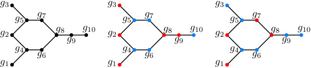 Figure 1
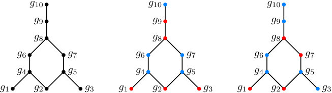 Figure 2
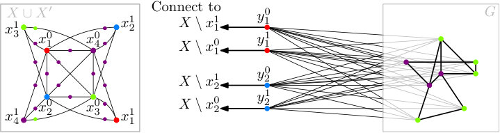 Figure 3
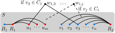 Figure 4
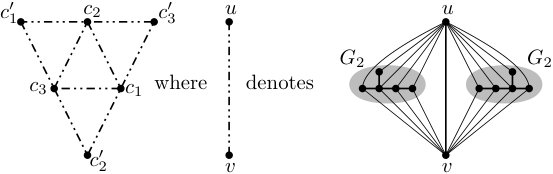 Figure 5
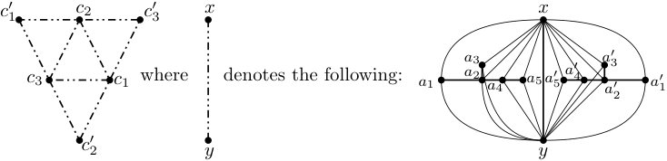 Figure 6
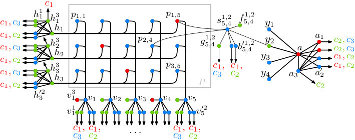 Figure 7
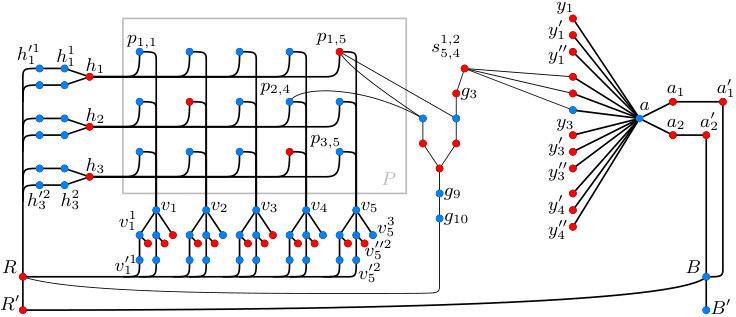 Figure 8
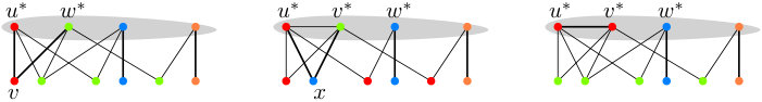 Figure 9
Peer Reviews
No public reviews on file for this paper yet. If you reviewed it on a platform where reviews are public (OpenReview, ICLR, NeurIPS, ICML), you can paste yours below so the community can read it here.
Videos
No videos yet. Explain this paper in a talk, walkthrough, or lecture? Add one.
11institutetext: Utrecht University, Netherlands. 11email: [email protected] 22institutetext: Ben Gurion University of Negev, Israel. 22email: [email protected]
33institutetext: Eindhoven University of Technology, Netherlands. 33email: [email protected]
Parameterized Complexity of Conflict-free Graph Coloring††thanks: This research was done with support by the NWO Gravitation grant NETWORKS. The research was partially done when the first and second author were associated with Eindhoven University of Technology.
Hans L. Bodlaender 11
Sudeshna Kolay 22
Astrid Pieterse 33
Abstract
Given a graph , a -open neighborhood conflict-free coloring or -ONCF-coloring is a vertex coloring such that for each vertex there is a vertex in that is uniquely colored from the rest of the vertices in . When we replace by the closed neighborhood , then we call such a coloring a -closed neighborhood conflict-free coloring or simply -CNCF-coloring. In this paper, we study the NP-hard decision questions of whether for a constant an input graph has a -ONCF-coloring or a -CNCF-coloring. We will study these two problems in the parameterized setting. First of all, we study running time bounds on FPT-algorithms for these problems, when parameterized by treewidth. We improve the existing upper bounds, and also provide lower bounds on the running time under ETH and SETH. Secondly, we study the kernelization complexity of both problems, using vertex cover as the parameter. We show that both -ONCF-coloring and -CNCF-coloring cannot have polynomial kernels when parameterized by the size of a vertex cover unless . On the other hand, we obtain a polynomial kernel for -CNCF-coloring parameterized by vertex cover. We conclude the study with some combinatorial results. Denote and to be the minimum number of colors required to ONCF-color and CNCF-color , respectively. Upper bounds on with respect to structural parameters like minimum vertex cover size, minimum feedback vertex set size and treewidth are known. To the best of our knowledge only an upper bound on with respect to minimum vertex cover size was known. We provide tight bounds for with respect to minimum vertex cover size. Also, we provide the first upper bounds on with respect to minimum feedback vertex set size and treewidth.
Keywords:
Conflict-free coloring, kernelization, fixed-parameter tractability, combinatorial bounds
1 Introduction
Often, in frequency allocation problems for cellular networks, it is important to allot a unique frequency for each client, so that at least one frequency is unaffected by cancellation. Such problems can be theoretically formulated as a coloring problem on a set system, better known as conflict-free coloring [7]. Formally, given a set system , a -conflict-free coloring is a function where for each set , there is an element such that for all , . In other words, each set has at least one element that is uniquely colored in the set. This variant of coloring has also been extensively studied for set systems induced by various geometric regions [2, 12, 20].
A natural step to study most coloring problems is to study them in graphs. Given a graph , denotes the set of vertices of while denotes the set of edges in . A -coloring of , for is a function . The most well-studied coloring problem on graphs is proper-coloring. A -coloring is called a proper-coloring if for each edge , . In this paper, we study two specialized variants of -conflict-free coloring on graphs, known as -ONCF-coloring and -CNCF-coloring, which are defined as follows.
Definition 1
Given a graph , a -coloring is called a -ONCF-coloring, if for every vertex , there is a vertex in the open neighborhood such that for all . In other words, every open neighborhood in has a uniquely colored vertex.
Definition 2
Given a graph , a -coloring is called a -CNCF-coloring, if for for every vertex , there is a vertex in the closed neighborhood such that for all . In other words, every closed neighborhood in has a uniquely colored vertex.
Observe that by the above definitions, the -ONCF-coloring (or -CNCF-coloring) problem is a special case of the conflict-free coloring of set systems. Given a graph , we can associate it with the set system , where consists of the sets given by open neighborhoods (respectively, closed neighborhoods ) for . A -ONCF-coloring (or -CNCF-coloring) of then corresponds to a -conflict-free coloring of the associated set system.
Notationally, let denote the minimum number of colors required for a conflict-free coloring of a set system . Similarly, we denote by and the minimum number of colors required for an ONCF-coloring and a CNCF-coloring of a graph , respectively. The study of conflict-free coloring was initially restricted to combinatorial studies. This was first explored in [7] and [19]. Pach and Tardos [17] gave an upper bound of on for a set system when the size of is . In [17], it was also shown that for a graph with vertices . This bound was shown to be tight in [11]. Similarly, [5] showed that .
However, computing or is NP-hard. This is because deciding whether a -ONCF-coloring or a -CNCF-coloring of exists is NP-hard [10]. This motivates the study of the following decision problems under the lens of parameterized complexity.
-ONCF-Coloring
Input: A graph .
Question: Is there a -ONCF-coloring of ?
The -CNCF-Coloring problem is defined analogously.
Note that because of the NP-hardness for -ONCF-Coloring or -CNCF-Coloring even when , the two problems are para-NP-hard under the natural parameter . Thus, the problems were studied under structural parameters. Gargano and Rescigno [10] showed that both -ONCF-Coloring and -CNCF-Coloring have FPT algorithms when parameterized by (i) the size of a vertex cover of the input graph , (ii) and the neighborhood diversity of the input graph. Gargano and Rescigno also mention that due to Courcelle’s theorem, for a non-negative constant , the two decision problems are FPT with the treewidth of the input graph as the parameter.
Our Results and Contributions.
In this paper, we extend the parameterized study of the above two problems with respect to structural parameters. Our first objective is to provide both upper and lower bounds for FPT algorithms when using treewidth as the parameter (Section 3). We show that both -ONCF-Coloring and -CNCF-Coloring parameterized by treewidth can be solved in time . On the other hand, for , both problems cannot be solved in time under Strong Exponential Time Hypothesis (SETH). For , both problems cannot be solved in time under Exponential Time Hypothesis (ETH).
We also study the polynomial kernelization question (Section 4). Observe that both -ONCF-Coloring and -CNCF-Coloring cannot have polynomial kernels under treewidth as the parameter, as there are straightforward and-cross-compositions from each problem to itself.111This is true for a number of graph problems when parameterized by treewidth. For more information, see [6, Theorem 15.12] and the example given for Treewidth (parameterized by solution size) in [6, page 534]. Therefore, we will study the kernelization question by a larger parameter, namely the size of a vertex cover in the input graph. The kernelization complexity of the -Coloring problem (asking for a proper-coloring of the input graph) is very well-studied for this parameter, the problem admits a kernel of size [14] which is known to be tight unless [13]. From this perspective however, -CNCF-Coloring and -ONCF-Coloring turn out to be much harder: -CNCF-Coloring for and -ONCF-Coloring for do not have polynomial kernels under the standard complexity assumptions, when parameterized by the size of a vertex cover. Interestingly, -CNCF-Coloring parameterized by vertex cover size does have a polynomial kernel and we obtain an explicit polynomial compression for the problem. Although this does not lead to a polynomial kernel of reasonable size, we study a restricted version called -CNCF-Coloring-VC-Extension (Section 4.4) and show that this problem has a kernel where is the vertex cover size. Therefore, -CNCF-Coloring behaves significantly differently from the other problems.
Finally, we obtain a number of combinatorial results regarding ONCF-colorings of graphs. Denote by the minimum for which a -proper-coloring for exists. While , the same upper bound does not hold for [10]. For a graph , let , and denote the size of a minimum vertex cover, the size of a minimum feedback vertex set and the treewidth of , respectively. From the known result that , we could immediately obtain the fact that the same behavior holds for . However, to show that behaves similarly more work needs to be done. To the best of our knowledge no upper bounds on with respect to and were known, while a loose upper bound was provided with respect to in [10]. We give a tight upper bound on with respect to and also provide the first upper bounds on with respect to and (Section 5).
Our main contributions in this work are structural results for the conflict-free coloring problem, which we believe gives more insight into the decision problems on graphs. Firstly, the gadgets we build for the ETH-based lower bounds could be useful for future lower bounds, but are also useful to understand difficult examples for conflict-free coloring which have not been known in abundance so far. We are able to reuse these gadgets in the constructions needed to prove the kernelization lower bounds. Secondly, our combinatorial results also give constructible conflict-free colorings of graphs and therefore provide more insight into conflict-free colored graphs. Finally, the kernelization dichotomy we obtain for -ONCF-Coloring and -CNCF-Coloring under vertex cover size as a parameter is a very surprising one.
2 Preliminaries
For a positive integer , we denote the set in short with . For a graph , given a -coloring and a subset , we denote by the restriction of to the subset . For a graph that is -ONCF-colored by a coloring , for a vertex , suppose is such that for each ; then is referred to as the ONCF-color of . Similarly, for a graph that is -CNCF-colored by a coloring , for a vertex , a unique color in is referred to as the CNCF-color of .
An edge-star graph is a generalization of a star graph where there is a central edge and all other vertices have . A triangle is an example of an edge-star graph.
2.1 Tree decompositions and treewidth
We define treewidth and tree decompositions.
Definition 3 (Tree Decomposition [6])
A tree decomposition of a (undirected or directed) graph is a tuple , where is a tree in which each vertex has an assigned set of vertices (called a bag) such that the following properties hold:
- •
.
- •
For any , there exists a such that .
- •
If and , then for all on the path from to in .
In short, we denote as .
The treewidth of a tree decomposition is the size of the largest bag of minus one. A graph may have several distinct tree decompositions. The treewidth of a graph is defined as the minimum of treewidths over all possible tree decompositions of . Note that for the tree of a tree decomposition, we denote a vertex of in bold font. If is rooted at a vertex , for a vertex , , where is the subtree rooted at .
A tree decomposition is called a nice tree decomposition if is a tree rooted at some node where , each node of has at most two children, and each node is of one of the following kinds:
- •
Introduce node: a node that has only one child where and .
- •
Forget vertex node: a node that has only one child where and .
- •
Join node: a node with two children and such that .
- •
Leaf node: a node that is a leaf of , and .
One can show that a tree decomposition of width can be transformed into a nice tree decomposition of the same width and with nodes, see e.g. [6].
We modify the definition of a nice tree decomposition slightly by ensuring that no bag in the tree decomposition is empty. This can easily be done by adding an arbitrary vertex to all bags of the current nice tree decomposition. This will ensure the non-emptiness property. Note that our nice tree decomposition will have width .
2.2 Parameterized complexity
Let be a finite alphabet. A parameterized problem is a subset of .
Definition 4 (Kernelization)
Let be two parameterized problems and let be some computable function. A generalized kernel from to of size is an algorithm that given an instance , outputs in time such that (i) if and only if , and (ii) and .
The algorithm is a kernel if . It is a polynomial (generalized) kernel if is a polynomial in .
Next, we describe a few methods that can be used to rule out the existence of polynomial kernels. One such method is by a polynomial parameter transformation [4] from a problem that is known to not admit a polynomial kernel. We repeat the necessary information here for completeness.
Definition 5 (Polynomial parameter transformation [4])
Let and be parameterized problems. A polynomial parameter transformation from to is an algorithm that takes an input and outputs such that the following hold.
- •
if and only if , and
- •
is bounded by a polynomial in .
We denote this as .
The following Theorem follows from [3, Prop. 2.16] and shows how to obtain lower bounds using polynomial parameter transformations.
Theorem 2.1 ([3])
Let and be parameterized problems with . If admits a polynomial generalized kernel, then admits a polynomial generalized kernel.
Another way to rule out the existence of polynomial kernels is using the framework of cross-compositions [3]. We start by providing the necessary definitions.
Definition 6 (Polynomial equivalence relation [3])
An equivalence relation on is called a polynomial equivalence relation if the following two conditions hold:
- •
There is an algorithm that given two strings decides whether and belong to the same equivalence class in time polynomial in .
- •
For any finite set the equivalence relation partitions the elements of into a number of classes that is polynomially bounded in the size of the largest element of .
Definition 7 (Cross-composition [3])
Let be a language, let be a polynomial equivalence relation on , and let be a parameterized problem. An or-cross-composition of into (with respect to ) is an algorithm that, given instances of belonging to the same equivalence class of , takes time polynomial in and outputs an instance such that the following hold:
- •
The parameter value is polynomially bounded in , and
- •
The instance is a yes-instance for if and only if at least one instance is a yes-instance for .
The following theorem shows how cross-compositions are used to prove kernelization lower bounds.
Theorem 2.2 ([3])
If an NP-hard language or-cross-composes into the parameterized problem , then does not admit a (generalized) polynomial kernelization unless .
2.3 Fast Subset Convolution Computation.
Given a universe with elements, the subset convolution of two functions is a function such that for every , . Equivalently, .
Proposition 1 ([8])
For two functions , given all the values of and in the input, all the values of the subset convolution can be computed in arithmetic operations.
In fact, this result can be extended to subset convolution of functions that map to any ring, instead of [6]. Consider the set , with the added relation that . The operator takes two elements from this set and outputs the maximum of the two elements. Notice that , along with as an additive operator and as a multiplicative operator, forms a semi-ring [6]. We will call this semi-ring the integer max-sum semi-ring. The subset convolution of two functions , with and as the additive and multiplicative operators, becomes .
Proposition 2 ([8])
Given two functions , all the values of and in the input, and all the values of the subset convolution over the integer max-sum semiring can be computed in time .
For more details about subset convolutions and fast calculations of subset convolutions, please refer to [6, 8].
3 Algorithmic results parameterized by treewidth
In this section, we state the algorithmic results obtained for the ONCF-Coloring and CNCF-Coloring problems parameterized by treewidth. On the algorithmic side, we have the following theorem.
Theorem 3.1
-ONCF-Coloring and -CNCF-Coloring parameterized by treewidth admits a time algorithm.
We also obtain algorithmic lower bounds for the problems under standard assumptions.
Theorem 3.2
The following algorithmic lower bounds can be obtained:
For , -ONCF-Coloring or -CNCF-Coloring parameterized by treewidth cannot be solved in time, under SETH. 2. 2.
-ONCF-Coloring or -CNCF-Coloring parameterized by treewidth cannot be solved in time, under ETH.
In the remainder of this section, we will prove the two theorems stated above.
3.1 Algorithms
In this section, we prove Theorem 3.1. In the following Lemma, we describe an algorithm for -ONCF-Coloring, parameterized by treewidth. The algorithm for -CNCF-Coloring parameterized by treewidth is very similar and has the same running time.
Lemma 1
-ONCF-Coloring parameterized by treewidth admits a time algorithm.
Proof
We assume that a nice tree decomposition , rooted at a leaf , is given to us. Also, recall that no bag in empty, and that each leaf bag or the root bag has exactly one vertex in it. We proceed with the following treewidth dynamic programming. Given a bag corresponding to the vertex , a state for the bag is a tuple , where
- •
determines the bag,
- •
is a vertex coloring of . Intuitively, for a vertex , is the color receives in the conflict-free coloring we are after.
- •
is a color assignment to each vertex of . For a vertex , should be the color that occurs exactly once in the neighborhood of .
- •
is an indicator function for the vertices of . The idea is that indicates whether already has a neighbor of color in the subtree rooted at i.
Let be the set of all states associated with . A function is defined as follows: For a state , suppose there is a vertex coloring such that (i) its restriction to the vertices in is the coloring , (ii) for each , the color is used at most once in , (iii) for each , if there is a a vertex such that then and otherwise , (iv) for any vertex , has a uniquely colored vertex under coloring . Then . Otherwise, . In other words, is such that except for the vertices in the graph induced on is ONCF-colored and a state stores a snapshot of at the boundary of the graph seen so far.
Our dynamic programming will calculate the function for each bag . Note that for the root , if in there is a state such that and , then the graph has a -ONCF-coloring. We describe our dynamic programming in cases according to the types of nodes of the tree decomposition.
Leaf Node:
Let be a leaf node. Then,
[TABLE]
This can be calculated in time. For the correctness, note that the uniquely colored neighbor of cannot appear in the graph seen so far as a leaf node only contains .
Forget Node:
Let be a forget node with its child being . Also, let . Consider a state and a state . We say that is consistent with , or if (i) , (ii) and . Then,
[TABLE]
This can be calculated in time. To prove correctness, first suppose and let be a coloring that is a witness to this. By definition of consistency, there is only one state such that . Since , the same coloring also witnesses the fact that . Conversely, suppose where is the unique state such that . Let be a coloring that is a witness to this. Since and by definition of consistency , the same coloring also witnesses the fact that . Thus, our recurrence correctly calculates .
Introduce Node:
Let be an introduce node with its child being . Also, let . Consider a state and a state . We say that is consistent with , or if (i) , (ii) if there is a such that then there is exactly one such and , otherwise there is no such and , (iii) If there is a such that then and , (iv) for all other , . Then,
[TABLE]
This can be calculated in time. To prove correctness, first suppose and let be a coloring that is a witness to this. By definition of consistency, there is at least one state such that and the same coloring also witnesses the fact that . Conversely, suppose there is a state such that and . Then by definition of consistency, . Thus, our recurrence correctly calculates .
Join Node:
Let be a join node with its children being and . This means that . Consider a state , and states . We say that is consistent with , or if (i) , (ii) if there is a such that () then () and , (iii) for all other , . Then,
[TABLE]
As before, the correctness of the recurrence follows from the definition of consistency.
It is straightforward to calculate this in time, we will further improve this to time as follows.
Notice that if we fix and , then get fixed for consistent states. Also, given , , and , consider the vertices . Then for each vertex , . Now consider . For consistent states, the following relations hold: (i) , (ii) and . Thus, if we are given the function , we can completely determine when we are looking at consistent states. Now, fix a function . We define functions in the following way. For a subset , define a function such that for any , and otherwise. Now, define and .
Then,
[TABLE]
The correctness of this recurrence is same as the correctness of the previous recurrence. Due to fast subset convolution over the max-sum semi-ring [6], this can be calculated in time. ∎
3.2 Running time lower bounds
In this section, we given the proof of Theorem 3.2 by describing lower bounds on algorithmic running times for the ONCF-Coloring and CNCF-Coloring problems parameterized by treewidth.
We start by providing a running time lower bound on -ONCF-Coloring under ETH claimed in Theorem 3.2. The bound will be obtained by giving a reduction from -SAT, and in order to give the reduction we will need the following type of gadget.
Definition 8
An ONCF-gadget is a gadget on ten vertices, as depicted in Figure 1.
The objective of this gadget is the following. The vertices in Figure 1 will be the interaction points of the ONCF-gadget with the outside world. As will be proved in the following two lemmas, the gadget is designed so as to (i) disallow certain -ONCF-colorings and (ii) allow certain -ONCF-colorings on its interaction points.
Lemma 2
Let be a ONCF-gadget with a coloring such that for all the neighborhood of is ONCF-colored by . If , then .
Proof
Suppose . Since , this implies . Similarly, we find . Since now has two blue vertices, we conclude that .∎
Lemma 3
Let be a ONCF-gadget. Let be a partial -ONCF-coloring of . If there exists such that , then can be extended to a coloring satisfying
For every , the neighborhood of vertex is ONCF-colored by (contains at most one red, or at most one blue vertex), and 2. 2.
, , , and .
Proof
Let equal on vertex and and define , , , and . If or , define else define . If or , define , otherwise let . This completes the definition of . It is easy to verify that both requirements are satisfied by this coloring, refer to Figure 1 for an example coloring.∎
Now that we have introduced the necessary gadgets, we can prove the running time lower bound for -ONCF-Coloring.
Lemma 4
-ONCF-Coloring parameterized by treewidth cannot be solved in time, under ETH.
Proof
We show this by giving a reduction from -SAT. Given an instance of -SAT with variables and clauses , create a graph as follows. Start by creating palette vertices , and , and edges and . For each variable , create vertices and add edges and . For the remainder of the construction we will reuse the ONCF-gadget as defined in Definition 8. For each , add an ONCF-gadget and connect of this gadget to . Add vertices , and and connect to in for . Let clause . Now if for some , connect to . Similarly, if , connect to . This concludes the construction of , it remains to show that is -ONCF-colorable if and only if the formula was satisfiable.
Suppose the satisfiability instance has satisfying assignment , we show how to color . Let , and . Let for all and define for all , . Finally, if , let and . Otherwise, let and . For each gadget , vertex for has neighbor . Let be the other neighbor of vertex . Define such that . Since the formula was satisfied by , for each there hereby exists such that . We use Lemma 3 to extend the partial coloring to color gadget , with and . It is straightforward to verify that is a -ONCF-coloring of .
Suppose has a -ONCF-coloring, we give a satisfying assignment . Assume without loss of generality that . Since for all , it follows that . We therefore define if and if . Let be a clause, we will show that satisfies to conclude the proof. Suppose for contradiction that does not satisfy . Then every vertex for had one neighbor in that is blue in . Thereby, its only other neighbor in gadget must be colored red. It follows from Lemma 2 that . Observe however that and that both these vertices are red, contradicting that is a -ONCF-coloring of . Thus, the formula is satisfied by .
Note that the graph induced by is a disjoint union of ONCF-gadgets and has treewidth two. As such, has treewidth at most .
In this reduction a -SAT formula on variables and clauses is reduced to a graph with treewidth at most . We proved that is satisfiable if and only if has a -ONCF-coloring. Since -SAT cannot be solved in time under ETH, this also implies that -CNCF-Coloring parameterized by treewidth cannot be solved in time, under ETH. ∎
Note that a reduction from -SAT to -ONCF-Coloring was given in Theorem 2 of [10]. However, that reduction led to a quadratic blow-up in the input size. Hence, the need for the alternative reduction given above.
Lemma 5
For , -ONCF-Coloring parameterized by treewidth cannot be solved in time, under SETH.
Proof
It was shown in [16] that for a constant , -Coloring cannot be solved in time, under SETH. For a graph , let be the graph obtained by subdiving every edge of once. It was shown in Theorem 3 of [10], that has a -coloring if and only if has a -ONCF-coloring. Also, note that since it is a subdivision of . Thus, for a constant , the lower bound of on the running time of any algorithm under SETH follows. ∎
Lemma 6
-CNCF-Coloring parameterized by treewidth cannot be solved in time, under ETH.
Proof
In [10], a reduction of -CNCF-Coloring was given from -SAT. In this reduction a -SAT formula on variables and clauses is reduced to a graph with treewidth at most . It was shown that is satisfiable if and only if has a -CNCF-coloring. Since -SAT cannot be solved in time under ETH, this also implies that -CNCF-Coloring parameterized by treewidth cannot be solved in time, under ETH. ∎
Lemma 7
For , -CNCF-Coloring parameterized by treewidth cannot be solved in time, under SETH.
Proof
It was shown in [16] that for a constant , -Coloring cannot be solved in time, under SETH. For a graph , Theorem 3.1 of [1] constructs a graph such that has a -coloring if and only if has a -CNCF-coloring. The construction of requires the graphs as described in Section 4.2, and first constructed in [1]. Recall that the is defined recursively as in Definition 9.
Returning to the construction of , we obtain from in the following manner: (i) for each vertex we add two copies and of and make adjacent to all vertices of and , (ii) for each edge we add two copies and of and make the vertices and adjacent to all vertices of and . This completes the construction of . For the completion of our proof it remains to show that in order to obtain a lower bound of on the running time of any algorithm under SETH.
Claim 1
For a graph , .
Proof
We prove our statement by induction on . In the base case, it is true that and . Let the induction hypothesis be that for any , . We prove the statement for . By construction, contains a clique on vertices. We create a bag with all the vertices of . By induction hypothesis, for each copy of we have a tree decomposition of width . Similarly, let be a tree decomposition of with width . Note that by construction, each copy of only has edges with a single vertex, say from the clique . To each bag of the corresponding tree decomposition, we add the vertex , thereby making the treewidth of the tree decomposition at most . We pick an arbitrary bag of the tree decomposition and attach it to the bag containing the vertices of . Similarly, each copy of only has edges with the end points of a single edge, say from the clique . To each bag of the corresponding tree decomposition, we add the vertices , thereby making the treewidth of the tree decomposition at most . We pick an arbitrary bag of the tree decomposition and attach it to the bag . The resulting tree decomposition has width at most . Thus, .
This helps us to show the desired treewidth bound for .
Claim 2
For a graph , .
Proof
The construction of a desired tree decomposition is similar to the construction given in the previous Claim. Let be a tree decomposition of . By construction, each copy of , that is added to to form , is attached to a single vertex in , say . From the previous Claim, we have a tree decomposition of width for this copy of . To each bag of , we add the vertex , thereby increasing the treewidth to at most . We pick an arbitrary bag of that contains and an arbitrary bag of and attach them together. Similarly, each copy of , that is added to to form , is attached to the end points of a single edge in , say . From the previous Claim, we have a tree decomposition of width for this copy of . To each bag of , we add the vertices , thereby increasing the treewidth to at most . We pick an arbitrary bag of that contains the edge and an arbitrary bag of and attach them together. Note that the resulting tree decomposition is a tree decomposition of and has width at most . Thus, we are done.
Thus, since is a constant. Thus, for a constant , the lower bound of on the running time of any algorithm under SETH follows. ∎
Thus, using Lemmas 4, 5, 7 and 6 we complete the proof of Theorem 3.2.
4 Kernelization
In this section, we will study the kernelizability of the ONCF- and CNCF-coloring problems, when parameterized by the size of a vertex cover. We prove the following two theorems to obtain a dichotomy on the kernelization question.
Theorem 4.1
-ONCF-Coloring for and -CNCF-Coloring for , parameterized by vertex cover size do not have polynomial kernels, unless .
Sections 4.1 and 4.2 together give a full proof of Theorem 4.1.
Theorem 4.2
-CNCF-Coloring parameterized by vertex cover size has a generalized kernel of size .
We prove the above theorem in Section 4.3. Note that by using an NP-completeness reduction, this results in a polynomial kernel for -CNCF-Coloring parameterized by vertex cover size. We also obtain an kernel for an extension problem of -CNCF-Coloring and this is described in Section 4.4.
4.1 Kernel lower bounds for -ONCF-Coloring
In this part, we begin the proof of Theorem 4.1 by showing that -ONCF-Coloring parameterized by vertex cover size has no polynomial kernel when is at least . We first show the relevant bound for and then use a polynomial parameter transformation to obtain the general lower bound.
For the construction in the following proof, we will again use the ONCF-gadget that was introduced in Definition 8 (and shown in Figure 1). Recall the relevant properties of this gadget that were given in Lemmas 2 and 3.
Lemma 8
-ONCF-Coloring parameterized by vertex cover size does not have a polynomial kernel, unless .
Proof
We show this by giving an or-cross-composition (see Definition 7) from Clique to -ONCF-Coloring parameterized by vertex cover size. Note that Clique is an NP-hard problem [9]. Therefore from Theorem 2.2, an or-cross-composition from Clique to -ONCF-Coloring parameterized by vertex cover size implies that the latter does not have a polynomial kernel unless .
We proceed with the description of the OR-cross-composition. For the sake of brevity, in this proof, we use -ONCF-coloring and ONCF-coloring interchangeably. We define a polynomial equivalence relation (see Definition 6) as follows. Let 2 instances of Clique be equivalent under if the graphs have the same number of vertices and they ask for a clique of the same size. It is easy to verify that is a polynomial equivalence relation. Suppose we are given instances of clique that are equivalent under , label them as . Let every instance have vertices and ask for a clique of size , enumerate the vertices in each instance arbitrarily. We create an instance for -ONCF-coloring by the following steps (see Figure 2 for a sketch of ).
Create vertices , , , and . Connect to , to and to . This ensures that and receive distinct colors in any coloring. (We will without loss of generality assume that receives the color red, and receives the color blue). Thus, the vertices and can be thought of as the palette for any -ONCF-coloring for . 2. 2.
Create vertices and let be the set containing these vertices. These vertices will be used to “select” which instance has a clique of size . 3. 3.
Add a vertex and connect to all vertices in . Add vertices , , , and and edges , , , and . Finally, connect to and connect to . This ensures that vertices and are red in any valid ONCF-coloring. Thereby, must have exactly one blue neighbor, implying exactly one vertex in is blue. The vertex that is colored blue in will then correspond to the input instance that has a clique of size . 4. 4.
Add vertices for , . Let be the set consisting of these vertices. These vertices will be used to select the vertices that correspond to a clique in one of the input instances. 5. 5.
Add a vertex for all . Connect to for all . For each vertex , add vertices , and . Connect to and . Connect to , connect to . Connect and to , in order to ensure that and will both be colored blue in any ONCF-coloring. Let be the set of all vertices created in this step. 6. 6.
Add a vertex for . Connect to for all . Create vertex and connect it to . Furthermore, create vertices , , and for all and connect to . Furthermore, connect to . Then, connect to and to for all . By this construction, vertex has at least two blue neighbors, and one neighbor whose coloring can be freely chosen. Let be the set of all vertices created in this step. 7. 7.
For every and , we add a vertex and let be the set containing all these vertices. For each , , and , add the edges , , and if and only if . The idea is that vertex verifies that if we select vertices and to be part of the clique, then no instance where can be selected as the yes-instance. To do this, we add additional gadgets in the following step. 8. 8.
For each and add a new ONCF-gadget . Identify vertex of the gadget with and identify vertex of the gadget with . Add the edge . Finally, connect vertex to .
In the remainder, we observe that for any -ONCF-coloring of . Thereby, we can safely rename the colors such that and .
Claim 3
Let be any -ONCF-coloring of , then , for all , and for all .
Proof
This follows immediately from the fact that there is a degree- vertex connecting these vertices to or respectively.
Claim 4
For any -ONCF-coloring of , there exists exactly one vertex such that and for all other vertices , .
Proof
Observe that and that by Claim 3. Thereby, must have a unique blue neighbor and this neighbor is in .
Claim 5
Let be a gadget and let be a -ONCF-coloring of . Then in this gadget implies that .
Proof
Suppose . It follows from Lemma 2 that thereby . Observe however that by definition. Since both these vertices are red, this contradicts the assumption that is a proper ONCF-coloring.
Claim 6
For any -ONCF-coloring of , there exist distinct such that and for all other , .
Proof
We start by showing that for each , there is exactly one such that . Consider the neighborhood of vertex . . Since by Claim 3, it follows that indeed contains exactly one red vertex, let this be vertex . It remains to show that all are distinct.
We show this by proving that for each , there is at most one such that . Consider vertex , observe that . Since by Claim 3, it follows that has a unique red neighbor, and thus there is at most one such that . Hereby, the claim follows.
Claim 7
If there exists an instance that has a clique of size , then can be -ONCF-colored.
Proof
Let be such that is a yes-instance for clique. Choose such that these vertices form a clique in . We now give an ONCF-coloring for , see Figure 2 for an example ONCF-coloring of .
Let and . 2. 2.
Let . For all other vertices in , let . 3. 3.
Let and . 4. 4.
Let for all . For all other vertices , let . 5. 5.
Let for all . Let for all other vertices . 6. 6.
For , let if , let otherwise. Let for all . Let for all remaining vertices . 7. 7.
Let for all . 8. 8.
It remains to color the introduced gadgets. Observe that vertices and of each gadget have already been colored, as they were identified with vertices from . We now proceed as follows. Define whenever has no blue neighbor in and define otherwise. Observe that since form a clique in instance , it never happens that by this definition. Color the remainder of each gadget using Lemma 3, such that the coloring satisfies property 2 of the lemma statement.
This defines a -coloring of , it remains to verify that is indeed a -ONCF-coloring. We consider the neighborhood of each vertex in .
. Since and for all , is ONCF-colored. , of which only is red. Thus, is ONCF-colored. Furthermore, and thereby it is trivially ONCF-colored, and which have distinct colors as desired. 2. 2.
For any vertex , contains vertex which is colored blue. Furthermore, and all vertices in are red. 3. 3.
. contains exactly one blue vertex, and and are colored red. , which have distinct colors as desired. Similarly, and these vertices are blue and red respectively. Finally, and , it is easy to verify that these are ONCF-colored. 4. 4.
For and , contains vertex which is red. Furthermore, only contains vertices from , which are blue, and vertices and from numerous ONCF-gadgets, which are also blue. Thereby it has red as a unique color in its neighborhood. 5. 5.
For , . Observe that all vertices in are blue, except vertex which is red. For , and these vertices receive distinct colors. and these vertices also receive distinct colors. 6. 6.
For , we observe that has exactly one red neighbor in and all its other neighbors are blue. Vertices and both have exactly one red neighbor, namely vertex or , respectively. Vertices have one blue and one red neighbor for . The vertices for and vertex have degree one and are thus ONCF-colored by definition. 7. 7.
For , , vertex has neighbors in and vertex in gadget . It follows from the definition of the coloring of and the fact that has at most one blue vertex that has exactly one blue neighbor. 8. 8.
It remains to verify that all gadget vertices are ONCF-colored properly, consider the vertices of gadget . The neighborhoods of vertices are ONCF-colored by definition. Vertices and were identified with vertices from and have already been discussed above. and these are blue and red, respectively. and these are also blue and red.
Claim 8
If can be -ONCF-colored, then there exists such that instance has a clique of size .
Proof
Let a -ONCF-coloring of be given. By Claim 4, there exists with . Pick such that . By Claim 6, take distinct such that . We will show that instance has a clique of size , by proving that vertices form a clique in .
Suppose not, then there exist such that and are not connected by an edge in . We show that this leads to a contradiction. Consider gadget . Vertices and of this gadget are colored red, as they were identified with vertices and respectively. It follows from Claim 5 that thereby in this gadget. Now consider the neighborhood of vertex . It contains vertex from gadget and the vertices since edge does not occur in instance . It now follows that vertex has at least two blue and two red neighbors in , which contradicts that is an ONCF-coloring of .
From Claims 7 and 8, it follows that can be -ONCF-colored if and only if there exists an such that has a clique of size . To prove the lower bound, it remains to bound the size of a vertex cover in . Since is an independent set in , it follows that is a vertex cover of . Observe that
[TABLE]
To conclude, since we have given a cross-composition from Clique to -ONCF-Coloring parameterized by vertex cover size, the lower bound now follows from Theorem 2.2.∎
Now, we use the lower bound obtained for -ONCF-Coloring in Lemma 8 and exhibit a polynomial parameter transformation to obtain the general lower bound for -ONCF-Coloring for all . This completes the lower bound results for -ONCF-Coloring claimed in Theorem 4.1.
Lemma 9
For any , -ONCF-Coloring parameterized by vertex cover size does not have a polynomial kernel, unless .
Proof
We prove the result by giving a polynomial parameter transformation from -ONCF-Coloring parameterized by vertex cover size to -ONCF-Coloring parameterized by vertex cover size for any constant . By Theorem 2.1 and Lemma 8, this implies that -ONCF-Coloring parameterized by vertex cover size, does not have a polynomial kernel unless for . We will do this by adding additional structures to the graph, that ensure that the original graph is colored using only colors, and that for any vertex in the original graph, its ONCF-color is also one of these two colors. Suppose we are given a graph for -ONCF-Coloring, we show how to obtain for -ONCF-Coloring.
Start by initiating as . Let . 2. 2.
Add vertices and . Let be the set of all these vertices. Add a clique on . Connect to for all with . Finally, subdivide all the edges between vertices in . (Thus, vertices form a subdivided clique in ). Let the set of vertices used to subdivide these edges be . 3. 3.
Add vertices for , let be the set containing all these vertices. Connect and to all vertices in . Then, connect to and connect to . Finally, connect and to every vertex . 4. 4.
For and , use a subdivided edge to connect to for all . Let be the set containing all vertices used for subdividing these edges. This ensures that always receives color .
Claim 9
If , then .
Proof
Suppose has a -ONCF-coloring , we will now show that has an -ONCF-coloring. It is easy to observe that for all , and furthermore for all , by the subdivided edges introduced in Step 2. By this observation, we may assume without loss of generality that . It is easy to observe using Step 4 of the construction, that in such a coloring . Thereby, for every , contains two vertices of color , for all . This implies that for any and , we know that is not the color that ensures that is -ONCF-colored.
Furthermore, contains two vertices of color for all (namely and ), and one vertex of color . Thereby, no vertex in can have color . This implies that only two colors are used in , namely and . We conclude that the coloring restricted to vertices in is a -ONCF-coloring for , after renaming the colors to .
Claim 10
If , then .
Proof
Suppose has a -ONCF-Coloring-coloring , we show how to -ONCF-color . First of all, let for all and let for all . For , let when and let otherwise. For the vertex on the subdivided edge from to , let . Similarly, for the vertex on the subdivided edge from to , let . For all remaining vertices, let . It remains to show that this gives a -ONCF-coloring of . See Figure 3 for a sketch of .
The neighborhoods of vertices in are trivially -ONCF-colored since they have no vertices of color or outside , and was a valid -ONCF-coloring. 2. 2.
For , vertex has exactly one neighbor of color , namely . For , vertices in have exactly one neighbor of color , namely or . Vertices in have degree and have neighborhoods that are -ONCF-colored by this definition. 3. 3.
Vertices and for each have exactly one neighbor of color and are thus -ONCF-colored. 4. 4.
Neighborhoods of the vertices used for subdividing edges always have two vertices of distinct color, by definition.
Since is a copy of to which we add additional vertices, it follows that the vertex cover of is bounded by where is the size of a vertex cover in . Thus, we have given a polynomial-parameter transformation from -ONCF-Coloring to -ONCF-Coloring with both problems having vertex cover size as parameter, and the theorem statement follows from Theorem 2.1 and Lemma 8.∎
4.2 Kernel lower bound for CNCF-Coloring
In this part, we complete the proof of Theorem 4.1 by showing that -CNCF-Coloring parameterized by vertex cover size has no polynomial kernel when is at least . To do this, we first introduce a useful gadget, which will serve as a color palette in our lower bound construction. The gadget is based on the graphs defined by Abel et al. [1, Section 3.1].
Definition 9 ([1])
For every positive integer , a graph is recursively defined as follows:
consists of a single isolated vertex. is a with one edge subdivided by another vertex (refer also to Figure 4). 2. 2.
Given and , is constructed as follows for :
- •
Take a complete graph on vertices.
- •
To each vertex , attach two disjoint and independent copies of , adding an edge from to every vertex of both copies of .
- •
For each edge , add two disjoint and independent copies of , adding an edge from and to every vertex of both copies.
Let denote the minimum number of colors needed to CNCF-color , when it is allowed to not color certain vertices. Abel et al. have shown the following lemma.
Lemma 10 ([1, Lemma 3.3])
For constructed in this manner, .
We use this to define the palette-gadget .
Definition 10
To create a palette-gadget start from a complete graph on vertices . Then, add vertices for and connect to for all . Let be the set of distinguished vertices of the gadget. Finally, for each edge with , add two new distinct copies of and connect all vertices in these copies to both and . See Figure 4 for an example of the palette-gadget .
The next two lemmas are used to establish that a palette gadget can indeed serve as a color palette for CNCF-Coloring.
Lemma 11
Let be a graph and let be a set of vertices such that is isomorphic to the palette-gadget for some . Let be a -CNCF-coloring of . Then for all with . Furthermore, for all .
Proof
We show this by showing that if is an edge such that there are two distinct copies of , say and , that are connected to both and and no other vertices in the graph, then in any -CNCF-coloring of . The results of the lemma statement then follow from the definition of the palette.
Suppose that for contradiction that there exists a -CNCF-coloring with . Let be a color such that . Observe that as and . Therefore, either or does not use color , w.l.o.g. let this be . We show that thereby , which contradicts Lemma 10.
Define partial coloring of as follows. For any with , let . For any with , leave undefined. Observe that hereby, the range of is a subset of and thus defines a -coloring of . From the correctness of and the fact that any vertex in has two neighbors of color under , it follows that is a partial -CNCF-coloring of , which is a contradiction. ∎
Lemma 12
Let be a palette-gadget for . Then there exists a -CNCF-coloring such that
* for all , and* 2. 2.
for all , contains exactly one vertex of color .
Proof
We start by defining for all . Let , observe that the color of all vertices in has now been defined. All vertices in induce distinct copies of . Consider an arbitrary copy of in , and suppose it was added to the palette gadget for the edge with . Color all vertices of this with a color such that . Observe that such a color exists since .
Both requirements are satisfied by the definition of , it remains to show that is a -CNCF-coloring of . Vertices and have color and have no neighbors of color , and are thereby properly CNCF-colored. Vertices in are distinct copies of . It is easy to verify that in there are two vertices with a unique color, corresponding to the edge for which it was added. Since these colors are not used to color , the result follows. ∎
Using the gadget introduced above, we now prove the kernelization lower bound.
Lemma 13
For any , -CNCF-Coloring parameterized by vertex cover size does not have a polynomial kernel, unless .
Proof
To prove this theorem, we will give a cross-composition starting from Clique that is very similar to the one given in Lemma 8.
We define the same polynomial equivalence relation; let two instances of Clique be equivalent if the graphs have the same number of vertices and they ask for a clique of the same size. Suppose we are given instances of clique that are equivalent under this relation, labeled . Let every instance have vertices and ask for a clique of size . We enumerate the vertices in each instance arbitrarily as . We create an instance for -CNCF-Coloring by the following steps, refer to Figure 5 for a sketch of .
Create a palette-gadget with distinguished vertices and by Definition 10. 2. 2.
Create vertices and let . The idea is that exactly one of these vertices will receive color in any -CNCF-coloring, and this indicates that is a yes-instance for clique. 3. 3.
Add a vertex and connect to for all . Create vertices and and connect both of these to vertices and in the palette-gadget. Furthermore, create vertices and and connect them to vertices and . Finally, create vertex , connect to , , , , and . Connect to , , , , and . The idea is that in any -CNCF-coloring, vertices and receive the color of , and receive the color of and that has exactly one neighbor of color and two neighbors of both remaining colors, implying that the color of cannot be . 4. 4.
Add vertices for all , . Let be the set containing all of these vertices. The idea is that vertices in receive colors and , such that for every there is exactly one vertex of color . The vertices of color will correspond to the vertices that form a clique in one of the input instances. 5. 5.
Add a vertex for all and connect to for all . Add vertices , , , and . Add edges , , , , , , , and . For all , add a vertex and connect it to . Connect to , , , and . Finally, connect to , , , , and . Let be the set of all vertices created in this step. These vertices will ensure that for each , there is exactly one vertex of color . 6. 6.
Add a vertex for all and connect to for all . Add vertices and and connect them to and . Add vertices and and connect these to and . Add a vertex . Finally, connect vertex to , , , , and . The vertices added in this step ensure that there cannot be such that both and receive color for some . 7. 7.
For each and , add vertex , let the set containing all these vertices be . Connect to and . Furthermore, connect to whenever is not an edge in instance . These vertices are used to verify whether the vertices selected by indeed form a clique in the selected input instance. 8. 8.
For each and , add vertices , , , and , and connect all these vertices to . Connect to and , connect to and , and finally connect to and . 9. 9.
For every vertex in , add the edges and for all . Thus, we connect every non-palette vertex in to all but the first three colors from the palette. This step ensures that colors are not used to color .
It follows from Lemma 11 that all receive distinct colors. Therefore, we will from now on assume that for any coloring . Furthermore, we observe that for , vertex is connected to and for all . It follows that vertex has its own color (if any) as its CNCF-color, since it is connected to two vertices of all remaining colors.
In the proofs of the remaining claims, we will regularly use that any non-palette vertex in has two neighbors of color for all .
Claim 11
For any -CNCF-coloring of , there exists exactly one vertex such that .
Proof
It follows from the observation above, that and . Furthermore, . Thereby, contains vertex , together with one vertex of color and two vertices of color for all , implying . It follows that contains at least two vertices of color and two of color and that contains no vertices of color . Thereby, must have exactly one vertex of color .
Claim 12
For any -CNCF-coloring of , there exist distinct such that and for all other , .
Proof
We start by showing that for each , there exists such that . We will then show that these are indeed distinct.
Let , then and thus contains two vertices of colors and . Since is connected to and contains at least one vertex of color , and two vertices of both color and , it follows that . Thereby, the CNCF-color for is and thus there exists a unique vertex in that receives color .
It remains to show that these are indeed distinct. We do this by showing that there cannot be vertices and such that . Suppose for contradiction that there are and such that . But then contains vertices and that have color , vertices and of color , and the aforementioned two vertices of color . Since it furthermore contains two vertices of color for all , this contradicts that is a CNCF-coloring for .
Claim 13
If there exists such that has a clique of size , then is -CNCF-colorable.
Proof
Take such that is a yes-instance for Clique and let be such that vertices form this clique in instance . We give a coloring of . We start by showing how to color the vertices defined in each step of the construction, this coloring is also depicted in Figure 5.
We start by coloring the palette as in Lemma 12, such that . 2. 2.
Let and for all other vertices . 3. 3.
Let and . 4. 4.
For all , let . For all other , let . 5. 5.
For all , let and let . 6. 6.
For all , let . For all , let and let . Let if there exists such that . Let otherwise. 7. 7.
For and , let . 8. 8.
For and , let , . Finally, if at this point has no neighbor of color , let . Furthermore, if is not connected to (meaning is an edge in ), define . Otherwise, let .
It remains to show that this indeed gives a -CNCF-coloring of . We verify this for all vertices. is CNCF-colored by the fact that and are colored by their own color and not connected to any other vertex of color . Vertices in are CNCF-colored by vertex which has color . contains exactly one vertex of color , namely . , and all contain exactly one vertex of color , namely . For , contains exactly one vertex of color and no other vertices of color . For all , contains exactly one vertex of color and not other vertices of color . Vertices , and have as their unique neighbor with color . Similarly, for all , the vertex has exactly one neighbor of color from the set . Vertices , and have as their only neighbor of color . Vertex has a distinct color from its only neighbor and thereby its closed neighborhood is CNCF-colored. Since and for all , , vertex receives a different color than its only neighbor. Vertices , , and all have a unique neighbor of color , namely vertex . Finally we check the closed neighborhood of vertices for , . If is not connected to , it is ensured that it has exactly one neighbor of color , namely vertex . Otherwise, observe that or as is not an edge in . The choice of coloring for ensures that in this case, has a unique neighbor of color .
Claim 14
If has a -CNCF-coloring, then there exists such that has a clique of size .
Proof
Let be a CNCF-coloring of . It follows from Claim 11 that there exists a vertex with . Let be such that . We show that has a clique of size . By Claim 12, there exist distinct such that . We show that the vertices form the desired clique in .
Suppose for contradiction that there are distinct such that is not an edge in instance . We will show that is not properly CNCF-colored. First of all, contains the two vertices and with . Furthermore it contains the two vertices and that have color , and finally it contains two vertices of color , namely and . Furthermore, contains two vertices of color for all , by Step 9 of the construction. This however contradicts that is a CNCF-coloring of , and thus we conclude that form a clique of size in instance .
It follows from Claims 13 and 14 that has a -CNCF-coloring if and only if one of the given input instances was a yes-instance for Clique. It remains to bound the size of a vertex cover in , to conclude the cross-composition. It is easy to verify that is a vertex cover for , since is an independent set. Thereby the size of a vertex cover in is at most , where is the size of palette-gadget . As this is properly bounded for a cross-composition, the theorem statement follows from Theorem 2.2. ∎
4.3 Generalized kernel for -CNCF-Coloring
In this part we prove Theorem 4.2, by obtaining a polynomial generalized kernel for -CNCF-Coloring parameterized by vertex cover size. This result is in contrast to the kernelization results we obtain for -CNCF-Coloring for as well as -ONCF-Coloring for . We will start by transforming an instance of -CNCF-Coloring to an equivalent instance of another problem, namely -Polynomial root CSP. We will then carefully rephrase the -Polynomial root CSP instance such that it uses only a limited number of variables, such that we can use a known kernelization result for -Polynomial root CSP to obtain our desired compression. We start by introducing the relevant definitions.
Define -Polynomial root CSP over a field as follows [15].
-Polynomial root CSP
Input: A list of polynomial equalities over variables . An equality is of the form , where is a multivariate polynomial over of degree at most .
Question: Does there exist an assignment of the variables satisfying all equalities (over ) in ?
A field is said to be efficient if both the field operations and Gaussian elimination can be done in polynomial time in the size of a reasonable input encoding. In particular, is an efficient field by this definition. The following theorem was shown by Jansen and Pieterse.
Theorem 4.3 ([15, Theorem 5])
There is a polynomial-time algorithm that, given an instance of -Polynomial root CSP over an efficient field , outputs an equivalent instance with at most constraints such that .
Using the theorem introduced above, we can now prove Theorem 4.2.
Proof (Proof of Theorem 4.2)
Given an input instance with vertex cover of size , we start by preprocessing . For each set with , mark vertices in with (if there do not exist such vertices, simply mark all). Let be the set of all marked vertices. Remove all with from . Let the resulting graph be .
Claim 15
* is -CNCF-colorable if and only if is -CNCF-colorable.*
Proof
In one direction, suppose has a -CNCF coloring using colors . Consider a vertex . Let be the neighborhood of . Note that is at most . Consider . Since was deleted, there are vertices in . Consider the color from that appears in majority on the vertices of . If we color with the same color, it is easy to verify that this extension of to is a -CNCF coloring of .
In the reverse direction, suppose has a -CNCF coloring using colors . We describe a new coloring for as follows. Consider a subset of size at most and let be the set of vertices in that have as their neighborhood. If and has a vertex that is uniquely colored in the set , then we arbitrarily choose a vertex . We define and . All other vertices have the same color in and . It is easy to verify that is also a -CNCF coloring of and the restriction of to is a -CNCF coloring of .
We continue by creating an instance of -Polynomial root CSP that is satisfiable if and only if is -CNCF-colorable. Let be the variable set. We create over as follows.
For each , add the constraint to . 2. 2.
For all , add the constraint 3. 3.
For each of degree add the constraint
[TABLE]
Note that such a constraint is a quadratic polynomial.
Intuitively, the first constraint ensures that every vertex is either red or blue. The second constraint ensures that in the closed neighborhood of every vertex, exactly one vertex is red or exactly one is blue. The third constraint is seemingly redundant, saying that the open neighborhood of every vertex outside the vertex cover does not have two red or two blue vertices, which is clearly forbidden. The requirement for these last constraints is made clear in the proof of Claim 18.
We show that this results in an instance that is equivalent to the original input instance, in the following sense.
Claim 16
* is a yes-instance of -Polynomial root CSP if and only if is -CNCF-colorable.*
Proof
Suppose is a satisfying assignment for . We show how to define a -CNCF coloring for . Let if and let if . Note that this defines exactly one color for each vertex, as by Step 1, and we used at most two distinct colors. It remains to show that this is indeed a CNCF-coloring. Let be an arbitrary vertex, we show that is conflict-free colored. It follows from the equations added in Step 2, that one of the following holds.
- •
. In this case, contains exactly one vertex with , showing that is conflict-free colored.
- •
. In this case, contains exactly one vertex with , showing that is conflict-free colored.
This concludes this direction of the proof.
For the other direction, suppose has -CNCF-coloring , we show how to define a satisfying assignment for . For , let if and let otherwise. Similarly, if and let otherwise. Observe that by this definition, for all , showing that we satisfy all equations introduced in Step 1. For the equations introduced in Step 2, consider an arbitrary vertex . Suppose its CNCF-color is red, then contains exactly one vertex with and thus , implying as desired. Similarly, if its CNCF-color is blue we obtain and again . It remains to prove that the equations added in Step 3 are satisfied. For this, let be an arbitrary vertex for which the equation was added. Observe that if is colored red, then its neighborhood contains no red vertices, such that and the equation is satisfied, or red vertices, such that and again the equation is satisfied. If is colored blue, then either its neighborhood is entirely red, such that or it contains exactly one red vertex, such that . In both cases the equation is satisfied.
Clearly, if is the number of vertices of . We will now show how to modify , such that it uses only variables for the vertices in . To this end, we introduce the following function. For , let f_{v}(V):=g\big{(}\sum\nolimits_{u\in N(v)}r_{u},|N(v)|\big{)}, where
[TABLE]
Note that for any fixed , describes a degree- polynomial in over . The following is easy to verify.
Observation 1
, and for all .
Observe that only uses variables defined for vertices that are in . As such, let , and let be equal to with every occurrence of for substituted by and every occurrence of for substituted by .
Claim 17
If is a satisfying assignment for , then is a satisfying assignment for .
Proof
We show this by showing that for all , in this case. Since by the constraints added in Step 1, this will conclude the proof. Consider an arbitrary vertex . Observe that by the equations added in Step 2, we are in one of the following cases.
- •
and . In this case, and thereby , by Observation 1.
- •
and . In this case, and thereby , using Observation 1.
- •
and . In this case, since for all , we obtain that , and thus . Thereby, by Observation 1.
- •
and . Hereby, and thus . Thus, using Observation 1.
The next claim shows the equivalence between and .
Claim 18
If is a satisfying assignment for , then there exists a satisfying assignment for such that .
Proof
Let be given, we show how to construct . For all , let . Furthermore, for , let and let . Since was simply obtained from by substituting by and by in all constraints, it is clear that satisfied all equations in . It remains to show that for all . If , this is obvious, so suppose such that . Observe that an equation was added for in Step 3. Therefore, we know that and it follows from Lemma 1 that takes a boolean value.
Using the method described above, we obtain an instance of -Polynomial root CSP such that has a satisfying assignment if and only if is -CNCF-colorable by Claims 15 and 16. Then we obtain an instance such that is satisfiable if and only if is satisfiable by Claims 17 and 18. As such, is a yes-instance if and only if is -CNCF-colorable and it suffices to give a kernel for . Observe that .
We start by partitioning into three sets , and . Let contain all equalities created for a vertex . Let contain all equations that contain at least one of the variables in and let contain the remaining equalities. Observe that by definition. Furthermore, the polynomials in have degree at most , as they were created for vertices in , and these are not connected. As such, we use Theorem 4.3 to obtain such that and any boolean assignment satisfying all equalities in satisfies all equalities in .
Similarly, we observe that by definition contains none of the variables in , implying that the equations in are equations over only variables. Since the polynomials in have degree at most , we can apply Theorem 4.3 to obtain such that and any assignment satisfying all equations in satisfies all equalities in .
We now define , and the output of our polynomial generalized kernel will be . The correctness of the procedure is proven above, it remains to bound the number of bits needed to store instance .
By this definition, . To represent a single constraint, it is sufficient to store the coefficients for each variable in . The storage space needed for a single coefficient is , as the coefficients are bounded by a polynomial in . Thereby, can be stored in bits. To bound this in terms of , we observe that it is easy to solve -CNCF-Coloring in time . This is done by guessing the coloring of , extending this coloring to the entire graph (observe has no vertices of degree less than three) and verifying whether this results in a CNCF-coloring. Therefore, we can assume that , as otherwise we can solve the -CNCF-Coloring problem in time, which is then polynomial in . Thereby we conclude that can be stored in bits. ∎
4.4 Kernelization bounds for conflict-free coloring extension
We furthermore provide kernelization bounds for the following extension problems.
-CNCF-Coloring-VC-Extension
Input: A graph with vertex cover and partial -coloring .
Question: Does there exist a -CNCF-coloring of that extends ?
We define -ONCF-Coloring-VC-Extension analogously.
We obtain the following kernelization results when parameterized by vertex cover size, thereby classifying the situations where the extension problem has a polynomial kernel. The extension problem turns out to have a polynomial kernel in the same case as the normal problem. However, we manage to give a significantly smaller kernel. Observe that the kernelization result is non-trivial, since -CNCF-Coloring-VC-Extension is NP-hard (see Theorem 4.5 below).
Theorem 4.4
The following results hold.
-CNCF-Coloring-VC-Extension* has a kernel with vertices and edges that can be stored in bits. Here is the size of the input vertex cover .* 2. 2.
-CNCF-Coloring-VC-Extension for any , and -ONCF-Coloring-VC-Extension parameterized by the size of a vertex cover do not have a polynomial kernel, unless .
We start by noting that the kernelization lower bounds given in the previous sections still apply. In particular, we obtain the following two Corollaries.
Corollary 1
-ONCF-Coloring-VC-Extension parameterized by the size of a vertex cover does not have a polynomial kernel, unless .
Proof
Observe that in the cross-composition given in Lemma 8, the vertices
[TABLE]
form a vertex cover of appropriately bounded size, and that these vertices receive always receive the same color in the proof of Claim 13. ∎
Furthermore, Lemma 13 immediately gives us the following result on this extension problem.
Corollary 2
For any , -CNCF-Coloring-VC-Extension parameterized by the size of a vertex cover does not have a polynomial kernel, unless .
Proof
The result follows immediately from the same cross-composition as given in the proof of Lemma 13. Observe that the vertices form a vertex cover of the created graph of size , and that they are always given the same coloring in the proof of Claim 13.∎
The results above prove part 2 of Theorem 4.4. We will now show that -CNCF-Coloring-VC-Extension has a simple polynomial kernel of size , where is the size of the vertex cover. This proves part 1 of Theorem 4.4. We start by arguing that -CNCF-Coloring-VC-Extension is indeed NP-hard.
Theorem 4.5
-CNCF-Coloring-VC-Extension is NP-hard.
Proof
We prove this by a reduction from Monotone Exact Sat, which is defined as follows.
Monotone Exact Sat
Input: A formula over variable set that is a conjunction of clauses, where each clause consists of a number of variables from .
Question: Does there exist an assignment such that every clause in contains exactly one variable that is set to ?
It is known that the Monotone Exact Sat problem is NP-hard, as it generalizes problem NP1 in [18]. Let an instance over variables be given, we show how to construct a graph with vertex cover and precoloring for -CNCF-Coloring-VC-Extension. See Figure 6 for a sketch of .
- •
Add vertices , , and to and to . Let and let . Connect to .
- •
For every clause in , add a vertex to . Let be contained in and let . Connect all vertices to .
- •
For every variable , add a vertex to , let be contained in and set . Connect to .
- •
For every , , if variable is in clause , construct a new vertex and connect to and . is not contained in .
Clearly, is hereby a vertex cover of and it is colored by . It is easy to see that the construction above can be done in polynomial time. It remains to show that can be extended to a -CNCF-coloring of if and only if is satisfiable.
Suppose is satisfiable and has satisfying assignment , we give a -CNCF-coloring of , such that extends . Naturally, for every vertex , let . For , let if and let otherwise. It remains to show that this is a valid CNCF-coloring of . We check the neighborhoods of all vertices.
. Here is a unique blue vertex. and is a unique red vertex in this set. and these vertices are red and blue, as desired. For any vertex , contains one blue vertex, namely where is such that is the unique variable in clause with . For any , . Since all vertices in receive the same color, this set has a uniquely colored vertex which is either (which is blue) or (which is red). For any , vertex has exactly two neighbors and these receive different colors, and thus is has a neighbor with a unique color.
Let be a CNCF-Coloring of . Let , then . Thereby, we observe that the vertices in all receive the same color since and . Let if all vertices in have color blue, and let otherwise. We show that is a satisfying assignment for . Let be a clause of , we show that there is exactly one such that , by showing that there is exactly one such that vertex . Consider vertex , then . Since since extends , it trivially follows that there is indeed a unique such that . This concludes the proof.∎
We now show that, unlike -CNCF-Coloring-VC-Extension, -CNCF-Coloring-VC-Extension has a simple polynomial kernel.
Lemma 14
-CNCF-Coloring-VC-Extension parameterized by the size of the vertex cover has a kernel of size .
Proof
Let with partial coloring and vertex cover be an instance of the problem, with . We first show how to obtain an equivalent instance such that and such that every vertex in has degree at most two. Then we can use a procedure given by Gargano and Rescigno [10] to further reduce the number of vertices in to at most .
If there exists a vertex that has at least two red and two blue neighbors by this precoloring, output a trivial no-instance. For the rest of the kernelization, we can thus assume that this case does not occur. Initialize as . Observe that for any vertex of degree at least , its coloring is now completely determined. While there exists a vertex of degree at least three in , we define as follows. If has only red neighbors, let . Otherwise, if has at least two red and exactly one blue neighbor, let . Similarly, if has only blue neighbors let and if has exactly one red neighbor let . It is easy to see that there is a -CNCF coloring of that extends , if and only if there is one extending .
For each vertex , mark two neighbors that are colored red by , and two that are blue (if these exist). Add all marked vertices to , and delete all vertices that have degree at least three and are not marked. Observe that hereby, is a coloring of the vertices of , is a vertex cover of , and each vertex in has degree at most two. We argue the following.
Claim 19
The graph has a -CNCF-coloring extension if and only if has a -CNCF-coloring extension.
Proof
Suppose has a -CNCF-coloring extension of , by the observation above there is also a -CNCF-extension of , let this be . We show that is a proper coloring of . Every vertex in has the same neighborhood as in , and thus this neighborhood is conflict-free colored by . For every vertex in , is the same in and . For the vertices in the color is the same for any -CNCF-coloring of and we kept two red and two blue vertices. As such, is a CNCF-coloring of .
Suppose has a -CNCF-coloring extension of . We define a -CNCF-coloring of that extends . Start by defining for any vertex . Hereby, all vertices in the vertex cover of are colored. Let . Note that has at least three neighbors in , as otherwise would have been a vertex in . Note that . Define as red if has only blue vertices. Furthermore, let if contains exactly one blue vertex. In all other cases, define . This concludes the definition of , it remains to show that is indeed a CNCF-coloring.
Clearly, by this definition, for any we have that is conflict-free colored by , as we assumed that no such vertex had two red and two blue neighbors. It remains to show that for , is conflict-free colored. Suppose for contradiction that it is not. Since any vertex was conflict-free colored by in , this implies that there exists a vertex that has two red and two blue neighbors under . Without loss of generality, suppose red was the conflict-free color of in . Thus, there is a vertex that is a neighbor of , with . But this contradicts that is removed by the marking procedure, as we always keep at least two red neighbors of if they exist. Thereby, is a CNCF-coloring of .
To obtain the kernel, for every set of size at most two, mark vertices with , if less than three such vertices exist, mark all. Remove all unmarked vertices from . This concludes the procedure. It follows from [10, Lemma 6] that this last step does not change the -CNCF-colorability of , observe that this still holds after predefining the coloring of the vertex cover. It is easy to observe that and . Furthermore, since any vertex in has degree at most two, . Using adjacency lists, this kernel can thus be stored in bits. ∎
This completes the proof of Theorem 4.4.
5 Combinatorial bounds
Given a graph , it is easy to prove that . However, there are examples that negate the existence of such bounds with respect to [10]. In this section, we prove combinatorial bounds for with respect to common graph parameters like treewidth, feedback vertex set and vertex cover.
First, note that if is a graph with isolated vertices then the graph can have no ONCF-coloring. Therefore, in all the arguments below we assume that does not have any isolated vertices. We obtain the following result. Recall that for a graph , , and denote the size of a minimum vertex cover, the size of a minimum feedback vertex set and the treewidth of , respectively.
Theorem 5.1
Given a connected graph ,
, 2. 2.
, 3. 3.
. Furthermore, if is not a star graph or an edge-star graph, then .
In order to prove the above theorem, we prove each item separately. In the following lemma, we consider the bound on with respect to the treewidth of a given graph.
Lemma 15
If is a graph with treewidth , then .
Proof
Consider a nice tree decomposition of . We give a vertex coloring of , which we will prove to be a -ONCF-coloring of . Furthermore, we give a function such that is the color that is uniquely used in the neighborhood of . We will color the graph such that
- •
If two vertices are in the same bag of , they receive distinct colors.
- •
The graph induced by the colored vertices is ONCF-colored, with the exception of vertices that are isolated.
Observe that by these two properties, is not only a ONCF-coloring, but also a proper coloring of .
Let an arbitrary leaf be the root, and let the corresponding bag be denoted as . Note that . Color each of the vertices in with a unique color from . For each vertex , if , pick one arbitrary vertex and let . Else, let .
Now, let be a vertex of such that its parent has been handled. We show how to color the vertices of . If , all vertices of have already been taken care of. Given that is a nice tree decomposition, the only alternative is is a forget node in . Hence, for some . Let and let . Since , it follows that . Thereby, . We color with a color from . If there is a vertex for which and , we let . Furthermore, if is not isolated in the graph constructed thus far, we let for some . Note that in the graph colored so far, .
We argue that is a -ONCF-coloring of . Consider a vertex . Let be the vertex that is a forget node for and that is closest to . By definition of a nice tree decomposition rooted at , is unique for the vertex . Let be the child of - by definition contains . Let be a bag closest to that contains both and a neighbor of . Then, by the definition of our coloring , there is a vertex that witnesses the conflict-free coloring of .
Thus, . ∎
A larger parameter than the treewidth of a graph is the size of a minimum feedback vertex set of a graph. In the following result, we compare with the size of a minimum feedback vertex set.
Lemma 16
If is a graph with a feedback vertex set of size , then .
Proof
Let be a FVS of size in . Using the color set , we define a vertex coloring , which we prove is a -ONCF-coloring of . The general idea is as follows. Vertices in are colored with , and vertices not in are conflict-free colored with . The only problem with this coloring are vertices in with no neighbors in . We resolve this issue by a careful recoloring of some of these vertices with color , and some of the vertices in with colors from .
Let . Initialize . Color the vertices in by the following procedure.
For all , let . 2. 2.
Each connected component of is a tree. If , then ONCF-color with colors and . Otherwise, (when ), color the single vertex in with . 3. 3.
while there exists such that 4. 4.
For each let 5. 5.
Let 6. 6.
Pick an arbitrary and let 7. 7.
for each 8. 8.
Let 9. 9.
If there is no , such that 10. 10.
Pick an arbitrary and recolor by letting
We argue that is a ONCF-coloring. We consider the different vertices in and argue their ONCF-coloring by . Let be the set as in line 7 of the procedure.
- •
Consider a vertex , if . In line 2, is given a conflict-free coloring using the colors , which are not used for vertices in . In line 9, some of these vertices may be recolored to for , but observe that any such color is used at most once in . This implies that is conflict-free colored by .
- •
For a vertex , if , then it cannot be the case that as this would contradict the while loop in the definition of the coloring. All other colors are used at most once on vertices in and therefore is ONCF-colored by .
- •
For a vertex , there is a neighbor in the color of which is unique in . Hence, is ONCF-colored by .
- •
Consider a vertex with . Note that . By definition of , there is a vertex and such that and . The color is used at most once in , and thus it is ONCF-colored by .
- •
Let be a vertex with . Note that . By definition of , there is a vertex that obtains a color , for some . Since color is used only once in , vertex witnesses the ONCF-coloring of .
Thus, . ∎
Observe that the bound given in Lemma 16 is close to being tight. If we start from a clique and subdivide each edge, the resulting graph has a feedback vertex set of size and needs colors to be ONCF-colored.
The next lemma bounds the value of for graphs with a vertex cover of size . In particular, we improve the bound given by Gargano and Rescigno [10, Lemma 4], who showed that .
Lemma 17
Let be a connected graph with . Then . Furthermore, if is not a star graph or an edge-star graph, then .
Proof
See Figure 7 for a sketch of the colorings described in the proof.
We start by proving the bounds for the case where is not a star and not an edge-star. Let be a minimum vertex cover of and let be the size of . We do a case distinction on the size and connectedness of .
( and connected) First, we prove the bounds for and is an edge . Note that is not an edge-star graph. Therefore at least one of or have neighbors with degree exactly in . We show that it is possible to ONCF-color such a graph with colors, namely and . Without loss of generality, let have degree- neighbor . We proceed as follows. Let , and . For any other vertex in , let . It remains to verify that this is a ONCF-coloring. Any is clearly ONCF-colored by the fact that their neighborhood is a subset of , and the vertices in receive different colors. Furthermore, has exactly one neighbor of color (namely ), and has one neighbor of color , namely , concluding this part of the proof.
( disconnected or ) We now prove the bounds for and is disconnected, and . We consider a number of cases.
(Suppose contains a connected component of size at least three.) Let be a vertex such that remains connected. We color the vertices in as follows. For every vertex , let . For every vertex that is isolated in , pick an arbitrary neighbor and (re)color such that . Notice that a vertex in may be picked multiple times as the candidate for an arbitrary neighbor for an isolated vertex in , and in this case the color of this vertex is set to the last color it is assigned. For every vertex that is not yet colored, let .
Note that by this definition, every vertex in has a distinct color. The colors that appear on vertices of are either or the color of a vertex that is isolated in . Also, by the choice of , every vertex in the component of has at least one other neighbor in . We verify that is an ONCF-coloring.
- •
From the above, every vertex that belongs to a connected component of size at least two in has a uniquely colored neighbor in S that witnesses the ONCF-coloring of . Note that this includes .
- •
Every isolated vertex in has . By description, every color for occurs at most once in , and sees at least one such vertex. Thus, is ONCF-colored.
- •
Finally, since all vertices in are distinctly colored, the neighborhoods of vertices in are ONCF-colored.
Also, notice that the number of colors used is . Thus, we are done in this case.
(Suppose only contains connected components of size one.) Note that . Start by letting for every vertex . Since is connected, there exists such that . Pick two vertices with . Let . For every vertex pick an arbitrary neighbor and recolor to . Color the vertices that remained uncolored by this procedure with . Note that by this procedure, every vertex in has a distinct color. To see that is a ONCF-coloring:
- •
Every vertex in has . By description, every color for occurs at most once in . Furthermore, has at least one neighbor with a color in . Thus, is ONCF-colored.
- •
Finally, since all vertices in are distinctly colored, the neighborhoods of vertices in are ONCF-colored.
Also, notice that the number of colors used is . Thus, we are done in this case.
(Otherwise.) In this case has size at least , contains multiple connected components, and at least one such component has size two. Let be a connected component in and let be another arbitrarily chosen vertex. We do a further case distinction.
- •
Suppose there exists a vertex with , take one arbitrary such vertex. Then we let for all , and we let . For every vertex that is isolated in , pick an arbitrary neighbor and recolor to . Define for all vertices that remained uncolored thus far. Notice that this coloring is very similar to the colorings in the previous cases. The only verification to be done is that for the sets and and both these neighborhoods have a vertex that is uniquely colored with . Thus, with arguments similar to those in the previous cases we obtain a -ONCF-coloring for in this case.
- •
Alternatively, if there exists no vertex with , then we let , and we let for all vertices in . For every vertex that is isolated in , pick an arbitrary neighbor and recolor to . Color all remaining vertices with . Notice that and have and uniquely colored with , respectively. Using arguments similar to previous cases, we can show that the described coloring is a -ONCF-coloring.
If is not a star and not an edge-star, we are in one of the cases above. Otherwise, it is easy to observe that stars have a vertex cover of size one and can always be colored with two colors, and edge-stars can be colored with three colors while having a minimum vertex cover size of two. ∎
Observe that the bounds of Lemma 17 are tight. First, a star graph requires colors and has vertex cover size while an edge-star graph requires colors and has vertex cover size . On the other hand, given an , taking the complete graph and subdividing each edge once results in a graph that requires colors [10] for an ONCF-coloring and has a vertex cover of size .
Using Lemmas 15, 16 and 17 we complete the proof of Theorem 5.1.
6 Open Problems
The study in this paper leads to some interesting open questions. In this paper we only exhibit a generalized kernel of size for -CNCF-Coloring and it remains to resolve the size of tight polynomial kernels for the problem. On the combinatorial side, with respect to minimum vertex cover, we obtain tight upper bounds on . It would be interesting to obtain corresponding tight bounds for with respect to feedback vertex set and treewidth.
The reference list from the paper itself. Each links out to its DOI / PubMed record.
- 1[1] Abel, Z., Alvarez, V., Demaine, E.D., Fekete, S.P., Gour, A., Hesterberg, A., Keldenich, P., Scheffer, C.: Three colors suffice: Conflict-free coloring of planar graphs. In: Proc. 28th SODA. pp. 1951–1963 (2017)
- 2[2] Ajwani, D., Elbassioni, K., Govindarajan, S., Ray, S.: Conflict-free coloring for rectangle ranges using O ( n .382 ) 𝑂 superscript 𝑛 .382 O(n^{.382}) colors. Discrete & Computational Geometry 48 (1), 39–52 (2012). https://doi.org/10.1007/s 00454-012-9425-5
- 3[3] Bodlaender, H.L., Jansen, B.M.P., Kratsch, S.: Kernelization lower bounds by cross-composition. SIAM J. Discrete Math. 28 (1), 277–305 (2014). https://doi.org/10.1137/120880240
- 4[4] Bodlaender, H.L., Thomassé, S., Yeo, A.: Kernel bounds for disjoint cycles and disjoint paths. Theor. Comput. Sci. 412 (35), 4570–4578 (2011). https://doi.org/10.1016/j.tcs.2011.04.039
- 5[5] Cheilaris, P.: Conflict-free Coloring. Ph.D. thesis, City University of New York (2009)
- 6[6] Cygan, M., Fomin, F.V., Kowalik, L., Lokshtanov, D., Marx, D., Pilipczuk, M., Pilipczuk, M., Saurabh, S.: Parameterized Algorithms. Springer (2015). https://doi.org/10.1007/978-3-319-21275-3
- 7[7] Even, G., Lotker, Z., Ron, D., Smorodinsky, S.: Conflict-free colorings of simple geometric regions with applications to frequency assignment in cellular networks. In: Proc. 43rd FOCS. pp. 691–700 (2002). https://doi.org/10.1109/SFCS.2002.1181994
- 8[8] Fomin, F.V., Kratsch, D.: Exact Exponential Algorithms. Springer (2010)