Warshall's algorithm -- survey and applications
Zolt\'an K\'asa

TL;DR
This paper surveys Warshall's algorithm, discussing its generalizations and various applications, providing a comprehensive overview of its utility in graph theory and related fields.
Contribution
It offers a comprehensive survey of Warshall's algorithm, including its generalizations and diverse applications, which was not extensively covered before.
Findings
Detailed overview of Warshall's algorithm and its variants
Examples of applications in graph connectivity and transitive closure
Identification of open problems and future research directions
Abstract
The survey presents the well-known Warshall's algorithm, a generalization and some interesting applications of this.
Click any figure to enlarge with its caption.
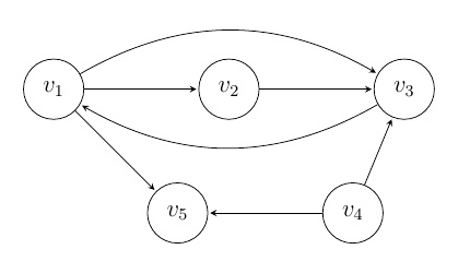 Figure 1
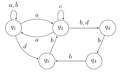 Figure 2
 Figure 1
 Figure 2
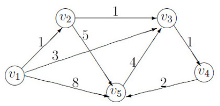 Figure 5
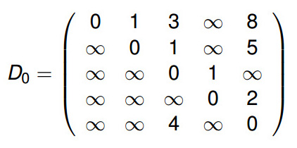 Figure 6
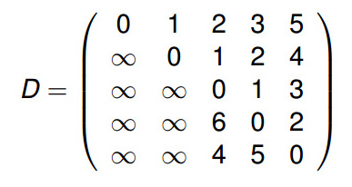 Figure 7
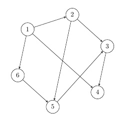 Figure 8
Peer Reviews
No public reviews on file for this paper yet. If you reviewed it on a platform where reviews are public (OpenReview, ICLR, NeurIPS, ICML), you can paste yours below so the community can read it here.
Videos
No videos yet. Explain this paper in a talk, walkthrough, or lecture? Add one.
Warshall’s algorithm—survey and applications
Abstract
The survey presents the well-known Warshall’s algorithm, a generalization and some interesting applications of this.
Zoltán KÁSA
Sapientia Hungarian University of Transylvania, Cluj-Napoca
Department of Mathematics and Informatics,
Tg. Mureş, Romania
1 Introduction
Let be a binary relation on the set , we write if is in relation to . The relation can be represented by the so called relation matrix, which is
[TABLE]
The transitive closure of the relation is the binary relation defined as:
if and only if there exists , , , such that , , . The relation matrix of is .
Let us define the following operations. If then for , and otherwise. for , and otherwise. In this case
[TABLE]
The transitive closure of a relation can be computed easily by the Warshall’s algorithm [6], [1]:
Warshall()
[TABLE]
A binary relation can be represented by a directed graph (i.e. digraph) too. he relation matrix is equal to the adjacency matrix of the corresponding graph. See Fig. 1 for an example. Fig. 2 represents the graph of the corresponding transitive closure relation.
2 Generalization of Warshall’s algorithm
Lines 5 and 6 in the Warshall’s algorithm described above can be changed in
[TABLE]
using the operations defined above. If instead of the operations + and we use two operations and from a semiring, a generalized Warshall’s algorithm results [4]:
Generalized-Warshall()
[TABLE]
This generalization leads us to a number of interesting applications.
3 Applications
3.1 Distances between vertices. The Floyd-Warshall’s algorithm
Given a weighted (di)graph with the modified adjacency matrix , we can obtain the distance matrix in which represents the distance between vertices and . The distance between vertices and is the length of the shortest path between them. The modified adjacency matrix is the following:
[TABLE]
Choosing for the operation (minimum between two reals), and for the real addition (), we obtain the well-known Floyd-Warshall’s algorithm as a special case of the generalized Warshall’s algorithm [4, 5] :
Floyd-Warshall()
[TABLE]
Figures 3 and 4 contain az example. The shortest paths can be easily obtained if in the description of the algorithm in line 5 we store also the previous vertex on the path. In the case of acyclic digraphs, the algorithm can be easily modified to obtain the longest distances between vertices, and consequently the longest paths.
3.2 Number of paths in acyclic digraphs
Here by path we understand directed path. In an acyclic digraph the following algorithm count the number of paths between vertices [3, 2]. The operation are the classical add and multiply operations for real numbers.
Warshall-Path()
[TABLE]
An example can be seen in Figures 5 and 6. For example between vertices 1 and 3 there are 3 paths: (1,2,3); (1,2,5,3) and (1,6,5,3).
3.3 All paths in digraphs
The Warshall’s algorithm combined with the Latin square method can be used to obtain all paths in a (not necessarily acyclic) digraph [3]. A path will be denoted by a string formed by its vertices in there natural order in the path.
Let us consider a matrix with the elements which are set of strings. Initially elements of this matrix are defined as:
[TABLE]
If and are sets of strings, will be formed by the set of concatenation of each string from with each string from , if they have no common elements:
[TABLE]
If is a string, let us denote by the string obtained from by eliminating the first character: . Let us denote by the set in which we eliminate from each element the first character. In this case is a matrix with elements
Operations are: the set union and set product defined as before.
Starting with the matrix defined as before, the algorithm to obtain all paths is the following:
Warshall-Latin()
[TABLE]
In Figures 7 and 8 an example is given. For example between vertices and there are two paths: and .
3.4 Scattered complexity for rainbow words
The application mentioned here can be found in [3]. Let be an alphabet, the set of all length- words over , the set of all finite word over .
Definition 1
Let and be positive integers, and . An -subword of length of is defined as where
,
* for ,*
**
Definition 2
The number of -subwords of a word for a given set is the scattered subword complexity, simply -complexity.
Examples. The word has 11 -subwords: , , , , , , , , , , . The -subwords of the word are the following: , , , , , , , , , , , , , , , , , , , .
Words with different letters are called rainbow words. The -complexity of a length- rainbow word does not depend on what letters it contains, and is denoted by .
To compute the -complexity of a rainbow word of length we will use graph theoretical results. Let us consider the rainbow word and the corresponding digraph , with
V=\big{\{}a_{1},a_{2},\ldots,a_{n}\big{\}},
E=\big{\{}(a_{i},a_{j})\mid j-i\in M,\,i=1,2,\ldots,n,j=1,2,\ldots,n\big{\}}.
For see Fig. 9.
The adjacency matrix A=\big{(}a_{ij}\big{)}_{\!\!\!\tiny\begin{array}[]{c}i\!\!=\!\!\overline{1,\!n}\\ j\!\!=\!\!\overline{1,\!n}\end{array}} of the graph is defined by:
[TABLE]
Because the graph has no directed cycles, the element in row and column in (where , with ) will represent the number of length- directed paths from to . If is the identity matrix (with elements equal to 1 only on the first diagonal, and 0 otherwise), let us define the matrix :
[TABLE]
The -complexity of a rainbow word is then
[TABLE]
Matrix can be better computed using the Warshall-Path algorithm.
From we obtain easily .
For example let us consider the graph in Fig. 9. The corresponding adjacency matrix is:
[TABLE]
After applying the Warshall-Path algorithm:
[TABLE]
and then K\big{(}6,\{2,3,4,5\}\big{)}=20, the sum of elements in .
Using the Warshall-Latin algorithm we can obtain all nontrivial (with length at least 2) -subwords of a given length- rainbow word . Let us consider a matrix with the elements which are set of strings. Initially this matrix is defined as:
[TABLE]
The set of nontrivial -subwords is .
For , the initial matrix is:
\left(\begin{array}[]{cccccccc}\emptyset&\emptyset&\emptyset&\{ad\}&\{ae\}&\{af\}&\{ag\}&\{ah\}\\ \emptyset&\emptyset&\emptyset&\emptyset&\{be\}&\{bf\}&\{bg\}&\{bh\}\\ \emptyset&\emptyset&\emptyset&\emptyset&\emptyset&\{cf\}&\{cg\}&\{ch\}\\ \emptyset&\emptyset&\emptyset&\emptyset&\emptyset&\emptyset&\{dg\}&\{dh\}\\ \emptyset&\emptyset&\emptyset&\emptyset&\emptyset&\emptyset&\emptyset&\{eh\}\\ \emptyset&\emptyset&\emptyset&\emptyset&\emptyset&\emptyset&\emptyset&\emptyset\\ \emptyset&\emptyset&\emptyset&\emptyset&\emptyset&\emptyset&\emptyset&\emptyset\\ \emptyset&\emptyset&\emptyset&\emptyset&\emptyset&\emptyset&\emptyset&\emptyset\\ \end{array}\right).
The result of the algorithm in this case is:
\left(\begin{array}[]{cccccccc}\emptyset&\emptyset&\emptyset&\{ad\}&\{ae\}&\{af\}&\{ag,adg\}&\{ah,adh,aeh\}\\ \emptyset&\emptyset&\emptyset&\emptyset&\{be\}&\{bf\}&\{bg\}&\{bh,beh\}\\ \emptyset&\emptyset&\emptyset&\emptyset&\emptyset&\{cf\}&\{cg\}&\{ch\}\\ \emptyset&\emptyset&\emptyset&\emptyset&\emptyset&\emptyset&\{dg\}&\{dh\}\\ \emptyset&\emptyset&\emptyset&\emptyset&\emptyset&\emptyset&\emptyset&\{eh\}\\ \emptyset&\emptyset&\emptyset&\emptyset&\emptyset&\emptyset&\emptyset&\emptyset\\ \emptyset&\emptyset&\emptyset&\emptyset&\emptyset&\emptyset&\emptyset&\emptyset\\ \emptyset&\emptyset&\emptyset&\emptyset&\emptyset&\emptyset&\emptyset&\emptyset\\ \end{array}\right).
3.5 Special paths in finite automata
Let us consider a finite automaton , where is a finite set of states, the input alphabet, the transition function, the initial state, the set of finale states. In following we do not need to mark the initial and the finite states.
The transition function can be generalized for words too: , where .
We are interesting in finding for each pair of states the letters for which there exists a natural such that we have the transition [4], i.e.:
[TABLE]
Instead of we use here set union () and instead of set intersection ().
Warshall-Automata()
[TABLE]
The transition table of the finite automaton in Fig. 10 is:
\begin{array}[]{c|cccc}\delta&a&b&c&d\\ \hline\cr q_{1}&\{q_{1},q_{2}\}&\{q_{1}\}&\emptyset&\{q_{5}\}\\ q_{2}&\{q_{1}\}&\{q_{3}\}&\{q_{2}\}&\{q_{3}\}\\ q_{3}&\emptyset&\{q_{4}\}&\emptyset&\emptyset\\ q_{4}&\emptyset&\{q_{5}\}&\emptyset&\emptyset\\ q_{5}&\emptyset&\{q_{2}\}&\emptyset&\emptyset\end{array}
Matrices for graph in Fig. 10 are the following:
A=\left(\begin{array}[]{ccccc}\{a,b\}&\{a\}&\emptyset&\emptyset&\{d\}\\ \{a\}&\{c\}&\{b,d\}&\emptyset&\emptyset\\ \emptyset&\emptyset&\emptyset&\{b\}&\emptyset\\ \emptyset&\emptyset&\emptyset&\emptyset&\{b\}\\ \emptyset&\{b\}&\emptyset&\emptyset&\emptyset\end{array}\right)
W=\left(\begin{array}[]{ccccc}\{a,b\}&\{a\}&\emptyset&\emptyset&\{d\}\\ \{a\}&\{a,b,c\}&\{b,d\}&\{b\}&\{b\}\\ \emptyset&\{b\}&\{b\}&\{b\}&\{b\}\\ \emptyset&\{b\}&\{b\}&\{b\}&\{b\}\\ \emptyset&\{b\}&\{b\}&\{b\}&\{b\}\\ \end{array}\right)
For example , , , for .
The reference list from the paper itself. Each links out to its DOI / PubMed record.
- 1[1] S. Baase, Computer Algorithms: Introduction to Design and Analysis, Second edition, Addison–Wesley, 1988.
- 2[2] C. Elzinga , H. Wang, Versatile string kernels , Theor. Comput. Sci. , 495, 1 (2013) 50–65.
- 3[3] Z. Kása , On scattered subword complexity missing 3, 1 (2011) 127–136.
- 4[4] P. Robert, J. Ferland, Généralisation de l’algorithme de Warshall, Revue Française d’Informatique et de Recherche Opérationnelle 2, 7 (1968) 71–85. http://www.numdam.org/item/?id=M 2AN_1968__2_1_71_0
- 5[5] Z. A. Vattai : Floyd-Warshall again, http://www.ekt.bme.hu/Cikkek/54-Vattai_Floyd-Warshall_Again.pdf
- 6[6] S. Warshall , A theorem on boolean matrices , Journal of the ACM , 9, 1 (1962) 11–12.