This paper investigates the stability of good quantum numbers, which are eigenvalues of a bounded self-adjoint operator commuting with the Hamiltonian, under perturbations, using order theory in quantum mechanics.
Contribution
It introduces a new perspective on the stability of quantum numbers by applying order theory to analyze perturbations of Hamiltonians with discrete spectra.
Findings
01
Good quantum numbers remain stable under certain perturbations.
02
Order theory provides a framework for analyzing eigenvalue stability.
03
Results have implications for understanding quantum state properties under perturbations.
Abstract
Let H be a self-adjoint operator, bounded from below and let O be a bounded self-adjoint operator with purely discrete spectrum. Suppose that (i) E(H)=infspec(H) is a simple eigenvalue, and (ii) H strongly commutes with O. Let ψH be the eigenvector associated with E(H). By the assumptions (i) and (ii), ψH is an eigenvector of O: OψH=μ(H)ψH. In the context of quantum mechanics, μ(H) is called a good quantum number. In this note, we examine the stability of μ(H) under perturbations of H from a viewpoint of the order theory.
\displaystyle\mathscr{P}_{\mathfrak{H}_{*},0}(O)=\{H\in\mathscr{P}_{\mathfrak{H}_{*},0}\,|\,\mbox{$e^{isO}e^{itH}=e^{itH}e^{isO}$ for all $s,t\in\mathbb{R}$}\}.
\displaystyle\mathscr{P}_{\mathfrak{H}_{*},0}(O)=\{H\in\mathscr{P}_{\mathfrak{H}_{*},0}\,|\,\mbox{$e^{isO}e^{itH}=e^{itH}e^{isO}$ for all $s,t\in\mathbb{R}$}\}.
No public reviews on file for this paper yet. If you reviewed it on a platform where reviews are public (OpenReview, ICLR, NeurIPS, ICML), you can paste yours below so the community can read it here.
Videos
No videos yet. Explain this paper in a talk, walkthrough, or lecture? Add one.
Taxonomy
TopicsSpectral Theory in Mathematical Physics · Quantum and electron transport phenomena · Quantum many-body systems
Full text
Stability of good quantum numbers in ground states
Let H be a self-adjoint operator, bounded from below and let O be a bounded self-adjoint operator
with purely discrete spectrum. Suppose that (i) E(H)=infspec(H) is a simple eigenvalue, and (ii)
H strongly commutes with O. Let ψH be the eigenvector associated with E(H). By the assumptions (i) and (ii), ψH is an eigenvector of O: OψH=μ(H)ψH.
In the context of quantum mechanics, μ(H) is called a good quantum number.
In this note,
we examine the stability of μ(H) under perturbations of H from a viewpoint of the order theory.
In addition, we provide some applications of the theory to the study of ferromagnetism.
Let H be a complex Hilbert space and let H be a self-adjoint operator on H, bounded from below.
Suppose that E(H)=infspec(H) is a simple eigenvalue, where spec(H) is spectrum of H. The eigenvector associated with E(H) is denoted by ψH.
Let O be a bounded self-adjoint operator with purely discrete spectrum.
Assume that H strongly commutes with O, that is, their spectral measures commute with each other.
Under this setting, we readily see that ψH is an eigenvector of O:
[TABLE]
In quantum mechanics, suppose that a particular Hamiltonian H and an operator O with corresponding eigenvalues and eigenvectors are given. Then the eigenvalues are said to be “good quantum numbers” if every eigenvector remains an eigenvector of the same eigenvalue as time evolves, or H strongly commutes with O.
In this sense, the eigenvalue μ(H) can be regarded as a good quantum number.
In this note, we will examine the stability of μ(H). To be precise, let V
be a self-adjoint operator.
We will consider a perturbation of H by V.
For simplicity, we suppose that V is bounded.
We continue to assume that
E(H+V) is a simple eigenvalue of H+V.
Our main purpose is to answer the following question.
*When does the equation μ(H+V)=μ(H) hold ?
*
In the rest of the present note, we will provide a framework which enables us to solve the above problem.
Our novel idea for constructing the framework is to apply the positivity improvingness of the resolvent of H.
Before we proceed, we briefly explain the motivation behind the aforementioned problem.
An essence of the problem originates from the study of ferromagnetism in many-electron systems;
Mathematical studies of ferromagnetism were initiated by Lieb [6], Nagaoka [12] and Thouless [16].
The origin of ferromagnetism still has been mystery and are actively examined even today, see e.g., [3, 4, 15].
In [8, 9, 10, 11], Miyao examined the stability of ferromagnetism in many-electron systems. In particular, he gave
a model independent framework which describes various stability results concerning
ferromagnetism in the Hubbard model [11].
Remark that in concrete applications to many-electron system, H corresponds to the Hamiltonian and O corresponds to the total spin operator.
In the present note, we focus our attention on a mathematical aspect of the theory established in [11]. We will find that its structure
is well decribed by the order theory.
The rest of the present note is organized as follows.
In Section 2, we introduce some basic notions to state our main result.
In particular, we focus our attention on the study of positivity improving resolvents.
In Section 3, we state our main result; we provide a novel framework which solve the stability problem stated in this introduction. Section 4 is devoted to give an example. This example suggests that our framework contains rich mathematical strucutures. In Appendices A
and B, we prove some operator inequalities which are useful in the main sections.
Acknowledgements
The author was partially supported by KAKENHI 18K03315.
2 Preliminary
2.1 Basic definitions
Let H be a complex Hilbert space.
By a convex cone, we understand a closed convex set P⊂H
such that tP⊆P for all t≥0 and P∩(−P)={0}.
The dual cone ofP is defined by
P†={η∈H∣⟨η∣ξ⟩≥0∀ξ∈P}.
We say that P is self-dual if
P=P†.
In what follows, we always assume that P is self-dual.
A vector ξ is said to be positive w.r.t. P if ξ∈P. We write this as ξ≥0 w.r.t. P.
A vector η∈P is called strictly positive
w.r.t. P whenever ⟨ξ∣η⟩>0 for all ξ∈P\{0}. We write this as η>0
w.r.t. P.
We denote by B(H) the set of all bounded linear operators on
H.
Definition 2.1
Let A∈B(H).
•
If AP⊆P,111
For each subset C⊆H, AC is
defined by AC={Ax∣x∈C}.
we then
write this as A⊵0 w.r.t. P. In
this case, we say that A* preserves the
positivity w.r.t. P.*
•
The set of all positivity preserving operators w.r.t. P is denoted by P(P).
P(P) is a weakly closed convex cone in B(H).
•
We write A⊳0 w.r.t. P, if Aξ>0 w.r.t. P for all ξ∈P\{0}.
In this case, we say that A* improves the
positivity w.r.t. P.*
Let L2(H) be the set of all Hilbert-Schmidt class operators on H.
It is well-known that L2(H) becomes a Hilbert space by introducing the norm
⟨A∣B⟩L2=tr[A∗B],A,B∈L2(H).
Let S(H) be the set of all density matries on H.222
We say that a linear operator ϱ on H is
a density matrix, if it is positive and trace class operator such that tr[ϱ]=1.
For given normalized vector ψ, we set ϱψ=∣ψ⟩⟨ψ∣. Trivially, we have ϱψ∈S(H). If ψ≥0 w.r.t. P, then ϱψ⊵0 w.r.t. P, while, if ψ>0 w.r.t. P, then ϱψ⊳0
w.r.t. P.
In the present note, we will examine self-adjoint operators satisfying the following conditions:
H is self-adjoint and bounded from below;
2.
H has purely discrete spectrum;
3.
(H+s)−1⊵0 w.r.t. P for all s>−E(H), where E(H)=infspec(H).
We denote by AP the set of all operators satisfying the conditions 1.-3. above.
Proposition 2.2
Let H,H′∈AP. If sH+tH′ is essentially self-adjoint for some s>0 and t>0, then
sH+tH′∈AP. In particular,
AP is a convex cone.
Proof.
By Proposition A.1, e−βsH⊵0 and e−βtH′⊵0 w.r.t. P for all β≥0.
By the Trotter product formula [13, Theorem S.20], we have
[TABLE]
where s-n→∞lim indicates the strong limit.
Because e−βsH/n⊵0 and e−βtH′/n⊵0 w.r.t. P, we see that
\big{(}e^{-\beta sH/n}e^{-\beta tH^{\prime}/n}\big{)}^{n}\unrhd 0 w.r.t. P for all β≥0 and n∈N. Thus, the right hand side of (2.2)
preserves the positivity w.r.t. P for all β≥0.
By applying Proposition A.1 again, we obtain that sH+tH′∈AP.
□
Let AP+ is the set of all self-adjoint operators satisfying 1., 2. and 3’. below:
3’.
(H+s)−1⊳0 w.r.t. P for all s>−E(H).
Remark 2.3
If H∈AP+, then E(H) is a simple eigenvalue with strictly positive eigenvector
by Theorem A.5.
**
2.2 Propagation of positivity
Let H1 and H2 be complex Hilbert spaces, and let P1 and P2 be self-dual cones in H1 and H2, respectively.
Suppose that H1 is a closed subspace of H2.
The orthogonal projection from H2 to H1 is denoted by π1,2.
We say that the *positivity is inherited from P1 to P2, * if
the following are satisfied:
P1=π1,2P2;
2.
π1,2⊵0 w.r.t. P2.
In this case, we write P1⇢P2. As we will see, this binary relation defines a partial order333Readers are referred to [14]
for partial orders..
The *conditional expectation * E1,2:B(H2)→B(H2) is defined by
Therefore, we have E1,2(π1,2P(P2)π1,2)⊆P(P1).
Conversely, suppose that A∈P(P1). Then, corresponding to the decomposition H2=H1⊕H1⊥, we have
A⊕0∈P(P2).
Indeed, for all x,y∈P2, we have
⟨x∣A⊕0y⟩=⟨π1,2x∣Aπ1,2y⟩≥0. Because E1,2(A⊕0)=A⊕0, we obtain that π1,2E1,2(P(P2))π1,2⊇P(P1). □
Definition 2.5
Let H1∈AP1 and H2∈AP2 be self-adjoint operators bounded from below.
If P1⇢P2 is satisfied, then we say that
*the P2-positivity of H2 is inherited from the P1-positivity of H1 * and write this as
(H1,P1)⇢(H2,P2).
**
Proposition 2.6
Suppose that (H1,P1)⇢(H2,P2).
Suppose that E(H1) and E(H2) are simple eigenvalues.
Then the corresponding eigenvectors, say ψH1 and ψH2, are positive, namely,
ψH1≥0 w.r.t. P1, and ψH2≥0 w.r.t.
P2. Equivalently, we have ϱψH1⊵0 w.r.t. P1 and ϱψH2⊵0 w.r.t. P2.
Moreover, π1,2E1,2(ϱψH2)π1,2⊵0 w.r.t. P1 and ⟨ψH1∣π1,2ψH2⟩≥0 hold.
Proof. By Proposition A.3, we have ψH1≥0 w.r.t. P1 and ψH2≥0 w.r.t. P2, respectively.
From the property P1=π1,2P2, it holds that π1,2ψH2≥0 w.r.t. P1.
Thus, we obtain that ⟨ψH1∣π1,2ψH2⟩≥0.
Because ϱψH2⊵0 w.r.t. P2, we obtain π1,2E1,2(ϱψH2)π1,2⊵0 by Proposition 2.4.
□
Let {Hn}n=1∞ be a sequence of Hilbert spaces, and let {Pn}n=1∞
and {Pn′}n=1∞ be
sequences of self-dual cones such that
(i)
Hn is a closed subspace of Hn+1;
(ii)
Pn and Pn′ are self-dual cones in Hn.
Assume that APn∩APn′={0} for all n∈N.
Suppose that a sequence of semibounded self-adjoint operators {Hn}n=1∞ satisfies the
following:
[TABLE]
By definition, we have ⟨ψH1∣π1,2ψH2⟩⟨ψH2∣π2,3ψH3⟩⋯⟨ψHn∣πn,n+1ψHn+1⟩≥0
and πj,j+1Ej,j+1(ϱψHj+1)πj,j+1⊵0
w.r.t. Pj, where πj,j+1 is the orthogonal projection from Hj+1 onto Hj.
In this sense, the positivity of ψH1 is propageted to ψHn for every n∈N.
2.3 Propagation of strict positivity
Definition 2.7
Let H1∈AP1+ and H2∈AP2+.
If P1⇢P2 is satisfied, then we say that *the strict
P2-positivity of H2 is inherited from the stirct P1-positivity of H1 * and write this as
(H1,P1)→(H2,P2). By definition, we readily confirm that if (H1,P1)→(H2,P2), then we have (H1,P1)⇢(H2,P2).
**
Let H1∈AP1+ and H2∈AP+. As before,
the ground state of Hj is denoted by ψHj,j=1,2.
Theorem 2.8
If (H1,P1)→(H2,P2), then
⟨ψH1∣π1,2ψH2⟩>0.
Equivalently,
we have \big{\langle}\varrho_{\psi_{H_{1}}}\big{|}\mathscr{E}_{1,2}(\varrho_{\psi_{H_{2}}})\big{\rangle}_{\mathscr{L}^{2}}>0. In addition, π1,2E1,2(ϱψH2)π2,1⊳0 w.r.t. P1.
To prove Theorem 2.8, we begin with the following lemma:
Lemma 2.9
Let A∈B(H) with A=0. Assume that u>0 w.r.t. P.
If A⊵0 w.r.t. P, then Au=0.
Proof.
First, we prove the following claim:
Let A∈B(H). If Au=0 for all u∈P, then A=0.
Indeed, by Proposition A.2, each u∈H can be written as
u=v1−v2+i(w1−w2), where v1,v2,w1,w2∈P such that ⟨v1∣v2⟩=0 and
⟨w1∣w2⟩=0. Thus, the assumption implies that Au=0
for allu∈H.
Assume that Au=0. Then, ⟨v∣Au⟩=0 for all v∈P,
implying that ⟨A∗v∣u⟩=0.
Since u>0 and A∗v≥0 w.r.t. P, we conclude that
A∗v must be zero. Because v is arbitrary,
A∗=0 by the above claim.
This contradicts with the assumption A=0.
□
Note that ψH1>0 w.r.t. P1 and ψH2>0 w.r.t. P2, respectively.
Because P1=π1,2P2 and π1,2⊵0 w.r.t. P2, we obtain that π1,2ψH2≥0 w.r.t. P1 and π1,2ψH2=0 by Lemma 2.9. Since ψH1>0 w.r.t. P1, we conclude that
⟨ψH1∣π1,2ψH2⟩>0.
For each x,y∈P\{0}, we have
⟨x∣E1,2(ϱψH2)y⟩=⟨x⊕0∣ψH2⟩⟨ψH2∣y⊕0⟩>0, which implies that π1,2E(ϱψH2)π1,2⊳0 w.r.t. P1.
□
As before, assume that APn∩APn′={0} for all n=1,…,N.
Suppose that a sequence of semibounded self-adjoint operators {Hn}n=1N satisfies the
following:
[TABLE]
Then, we have ⟨ψH1∣π1,2ψH2⟩⟨ψH2∣π2,3ψH3⟩⋯⟨ψHN−1∣πN−1,NψHN⟩>0 for each N∈N (equivalently,
\big{\langle}\varrho_{\psi_{H_{1}}}\big{|}\mathscr{E}_{1,2}(\varrho_{\psi_{H_{2}}})\big{\rangle}_{\mathscr{L}^{2}}\cdots\big{\langle}\varrho_{\psi_{H_{N-1}}}\big{|}\mathscr{E}_{N-1,N}(\varrho_{\psi_{H_{N}}})\big{\rangle}_{\mathscr{L}^{2}}>0)
by Theorem 2.8. Furthermore, πj,j+1Ej,j+1(ϱHj+1)πj,j+1⊳0 w.r.t. Pj for all j∈N.
In this sense, a strict positivity of ψH1 is propageted to ψHN.
As we will see in the following sections, this property is important to examine the stability of the good quantum numbers.
Definition 2.10
We say that (H1,P1) and (HN,PN′) are connected by
the sequences {(Hj,Pj)}j=1N−1 and {(Hj,Pj′)}j=2N if
(2.6) holds.
We simply express this as H1→HN.
**
For a given Hilbert space H∗, let HH∗ be the set of all Hilbert spaces containing
H∗ as a closed subspace. Let PH∗,0 be the set of self-adjoint operators defined by
[TABLE]
where the union ⋃P⊂H runs over all self-dual cones in H.
Proposition 2.11
The binary relation “ →” is a preoder on PH∗,0. Namely, we have the following:
(i)
H→H;
(ii)
H→H′,H′→H′′⟹H→H′′.
Proof. (i) Because H∈PH∗,0, there is a self-dual cone P such that
H∈AP+. Then we can readily check that (H,P)→(H,P).
(ii) By definition, H and H′ are connected by seqences P={(Hj,Pj)}j=1N−1 and P′={Hj,Pj′}j=2N
with H1=H and HN=H′. Also H′ and H′′ are connected by sequences
Q={(Kj,Qj)}j=1M−1 and Q′={(Kj,Qj′)}j=2M
with K1=H′ and KM=H′′.
Now we define new sequences R and R′ by R=P∪Q and R′=P∪Q′, then H and H′′ are connected by R and R′. □
Definition 2.12
Let H1,H2∈PH∗,0.
If H1→H2 and H2→H1, then we write this as H1≡H2.
The binary relation “ ≡ ” is an equivalence relation on PH∗,0.
Let PH∗,0 be the set of equivalence classes: PH∗=PH∗,0/≡.
The equivalence class containing H is denoted by [H].
The binary relation “→” on PH∗ is naturally defined by
[H1]→[H2]\mboxifH1→H2.
This is a partial order on PH∗; namely, we have, by Proposition 2.11,
(i)
[H]→[H];
(ii)
[H1]→[H2],[H2]→[H1]⟹[H1]=[H2];
(iii)
[H1]→[H2],[H2]→[H3]⟹[H1]→[H3].
In what follows, we abbreviate [H]→[H′] to H→H′ if no confusion arises.
**
3 Stability of good quantum numbers in ground states
3.1 Main result
Let O∈B(H∗) be self-adjoint.
In what follows, we always assume that O has purely discrete spectrum.
In this section, we will explore the following class of self-adjoint operators:
[TABLE]
For each H∈HH∗, O can be naturally extended to a self-adjoint operator on H.444
Indeed, corresponding to the decomposition H=H∗⊕H∗⊥,
the natural extension of O to H is defined by O⊕0. We denote by O this natural extension
if no confusion arises.
The natural extension is also denoted by the same symbol O.
Note that the preorder “→” can be defined on PH∗,0(O) as well.
As before, we set PH∗(O)=PH∗,0(O)/≡.
Then the preoder “→” can be also lifted up to a partial order.
We identify the equivalence class [H]∈PH∗(O) with H if no confusion occurs.
Proposition 3.1
Let H,K∈PH∗(O).
If H→K, then μ(H)=μ(K).
Proof. Suppose that H∈AP+ and K∈AQ+.
There exist sequences {(Hj,Pj)}j=1N−1 and {(Hj,Pj′)}j=2N satisfying (2.6) with H1=H,P1=P,HN=K and PN′=Q.
Let πj,j+1 be the orthogonal projection from Hj+1 onto Hj.
Let Ej,j+1 be the corresponding conditional expectation. Because O∈B(H∗),
we see that Ej,j+1(O)=O, which implies that
[TABLE]
By applying Theorem 2.8, we obtain that
μ(Hj)=μ(Hj+1). Repeating this argument several times, we arrive at
μ(H)=μ(H1)=μ(H2)=⋯=μ(HN)=μ(K). □
Definition 3.2
Let H∗∈PH∗(O). The H∗-stability classUO(H∗) is defined by
UO(H∗)={H∈PH∗(O)∣H∗→H}.
**
Theorem 3.3
For every Hamiltonian H∈PH∗(O) in the H∗-stability class, we have μ(H)=μ(H∗).
Proof. The theorem immediately follows from Proposition 3.1. □
3.2 Basic properties of UO(H∗)
In this subsection, we will prove two basic properties of
UO(H).
Theorem 3.4
For each H∈PH∗(O), the cardinality of UO(H) is greater than ℵ0,
the cardinality of the natural numbers. In this sense, UO(H) is rich.
Proof.
Suppose that H acts in the Hilbert space H. Note that because H∈PH∗(O),
there is a self-dual cone P in H such that H∈AP+.
We consider an extended Hilbert space H⊗C2.
We define a Hamiltonian H1 acting in H⊗C2 by
H1=H⊗1−1⊗σ1,
where σ1 is the standard Pauli matrix: σ1=(0110). Remark the following facts:
\mathbb{R}^{2}_{+}=\bigg{\{}\left(\begin{array}[]{c}x\\
y\end{array}\right)\in\mathbb{C}^{2}\,\bigg{|}\,x,y\geq 0\bigg{\}} is a self-dual cone in C2, and the lowest eigenvalue of −σ1
is simple with strictly positive eigenvector. Indeed, the eigenvector is given by \psi_{-\sigma_{1}}=\left(\begin{array}[]{c}1/\sqrt{2}\\
1/\sqrt{2}\end{array}\right), which is obviously strictly positive w.r.t. R+2.
Now we define a self-dual cone in H⊗C2 by
\mathfrak{P}_{1}=\bigg{\{}\Psi_{1}\otimes\left(\begin{array}[]{c}1\\
0\end{array}\right)+\Psi_{2}\otimes\left(\begin{array}[]{c}0\\
1\end{array}\right)\,\bigg{|}\,\Psi_{1},\Psi_{2}\in\mathfrak{P}\bigg{\}}.
Note that the ground state of H1 is unique and concretely given by ψH1=ψH⊗ψ−σ1.
Since H∈AP+, it holds that ψH>0 w.r.t. P. Thus, we readily confirm
that ⟨Φ∣ψH1⟩>0 for all Φ∈P1\{0}, which implies that ψH1>0
w.r.t. P1.
By applying Theorem A.5, we conlude that (H1+s)−1⊳0 w.r.t. P1 for all s>−E(H1).
We introduce an orthogonal projection P by P\Psi\otimes r=\Psi\otimes\left(\begin{array}[]{c}0\\
r_{2}\end{array}\right) for each Ψ∈H and r=\left(\begin{array}[]{c}r_{1}\\
r_{2}\end{array}\right)\in\mathbb{C}^{2}.
We can identify ran(P) with H
by the isometry \tau:\mathrm{ran}(P)\ni\Psi\otimes\left(\begin{array}[]{c}0\\
r_{2}\end{array}\right)\mapsto r_{2}\Psi\in\mathfrak{H}.
By definition, we have P⊵0 w.r.t. P1 and PP1=P by the aforementioned identification.
Hence, we readily check that H→H1.
Next, let us consider a further extended Hilbert space
(H⊗C2)⊗C2.
Define a Hamiltonian H2 by
H2=H1⊗1−1⊗σ1, and define a self-dual cone P2 by \mathfrak{P}_{2}=\bigg{\{}\Phi_{1}\otimes\left(\begin{array}[]{c}1\\
0\end{array}\right)+\Phi_{2}\otimes\left(\begin{array}[]{c}0\\
1\end{array}\right)\,\bigg{|}\,\Phi_{1},\Phi_{2}\in\mathfrak{P}_{1}\bigg{\}}. Using arguments similar to those in the last paragraph, we can confirm that H1→H2, which implies that H→H2.
Repeating this procedure, we can construct a sequence of Hamiltonians {Hℓ}ℓ=1∞ such that H→Hℓ.
Therefore, UO(H) contains at least countably infinite number of Hamiltonians. □
Proposition 3.5
Let UO be the set of all stability classes: UO={UO(H)∣H∈PH∗(O)}.
Then UO is a partially ordered set under set inclusion.
In addition, the map UO:PH∗(O)→UO is
monotonically decreasing, that is, if H1→H2, then UO(H1)⊇UO(H2).
Proof. Suppose that H∈UO(H2). Then we have H2→H. Because H1→H2,
we conclude that H1→H by Definition 2.12. Thus, H∈UO(H1), i.e., UO(H1)⊇UO(H2). □
3.3 Equivalent Hamiltonians
Let M∗ and N be von Neumann algebras on a separable Hilbert spaces H∗ and X, respectively.
Let Ω∗ and ΩX
be cyclic and separating vectors for M∗ and N, respectively.
We denote by P∗ and PX the natural cones associated with the pairs
{M∗,Ω∗} and {N,ΩX}, respectively.555
We use Δ and J to denote the modular operator and the modular conjugation associated with the pair {M,Ω}.
Let
P0(M)={AJAJ∣A∈M}.
The natural coneP associated with the pair {M,Ω} is defined by
P=P0(M)Ω,
where the bar denotes the strong closure.
It is well-known that P is a self-dual cone in H [1].
We set
[TABLE]
Because Ω is a cyclic and separating vector for M, we can also define the natural cone P associated with M.
Physically, X represents effects from environments surrounding the system described by M∗.
Let π=1⊗∣ΩX⟩⟨ΩX∣. Then π is
the orthogonal projection from H to H∗≅H∗⊗ΩX, where H∗⊗ΩX={φ⊗ΩX∣φ∈H∗}. Note that all results in the previous sections hold true for H1=H∗≅H∗⊗ΩX and H2=H.
For given Hamiltonian H∗ acting in H∗,
let us consider H∗-stability class UO(H∗).
Definition 3.6
We say that the Hamiltonian H is equivalent to H∗, if
there is a semibounded self-adjoint operator L on X
such that L∈APX+ and H=H∗⊗1+1⊗L.
**
Let H∈UO(H∗). Let ψ∗ and ψ be the normalized ground states of H∗ and H, respectively.
The following proposition is readily confirmed.
Proposition 3.7
Suppose that H is equivalent to H∗.
Then there exists a normailzed vector ω∈X such that
ψ=ψ∗⊗ω;
2.
ω>0* w.r.t. PX.*
Remark 3.8
Let {Hℓ}ℓ=1∞ be the sequence of Hamiltonians constructed in the proof of Theorem 3.4. By the construction, Hℓ+1 is equivalent to Hℓ for all ℓ∈N; thus, every Hℓ is equivalent to H. In this sense, this example is rivial.
As we will see in Section 4, we can construct sequences of Hamiltonians in UO(H) which are inequivalent to each other.
**
As before, we set ϱψ∗=∣ψ∗⟩⟨ψ∗∣ and ϱψ=∣ψ⟩⟨ψ∣.
Let trX be the partial trace operations trX:B(H)→B(H∗). We define a density matrix by ϱψH∗=trX[ϱψ].
The quantum relative entropy of ϱψH∗ to ϱψ∗ is given by
[TABLE]
Definition 3.9
We say that H∈UO(H∗) is weakly equivalent to H∗, if S(ϱψH∗∣ϱψ∗)=0.
**
Theorem 3.10
Let H∈UO(H∗). The following (i) and (ii) are equivalent:
(i)
H* is weakly equivalent;*
(ii)
There exists a normailzed vector ω∈X such that
ψ=ψ∗⊗ω;
2.
ω>0* w.r.t. PX.*
Remark 3.11
By Proposition 3.7, the triviality of H implies the condition (ii). However, the converse is false in general.
**
(i) ⇒ (ii): First, note that S(ϱψH∗∣ϱψ∗)=0 if and only if
ϱψH∗=ϱψ∗. Thus, there exists an x∈X such that ψ=ψ∗⊗x.
Because ψ and ψ∗ are strictly positive, x must be strictly positive. □
4 Example: construction of a lattice
In this subsection, we will
show that UO(H) is truly rich in the sense that UO(H)
contains infinitely many inequivalent Hamiltonians, and
illustrate the interesting structure of UO(H) by constructing a
specific example.
Let H0 be a self-adjoint operator on H∗, bounded from below.
In this section, we assume the following condition:
(H)e−βH0⊳0 w.r.t. P∗ for all β>0.
By Proposition A.4, we have H0∈AP∗+.
Suppose that H0 commutes with O.
Our purpose in this subsection is to examine the stability of μ(H0).
For each n∈N with n≥2, we consider a Hilbert space
H∗⊗Cn.
Then H∗
can be regarded as a closed subspace of H∗⊗Cn in the following manner:
H∗≅H∗⊗(1/n,…,1/n)T⊂H∗⊗Cn,
where aT indicates the transpose of a
and H⊗a={ψ⊗a∣ψ∈H}.
Thus, H∗⊗Cn∈HH∗.
A natural self-dual cone in H∗⊗Cn is given by
[TABLE]
where R+n is a natural self-dual cone in Cn: R+n={r=(r1,…,rn)T∈Rn∣rj≥0,j=1,…,n}, {ej}j=1n is a standard orthonormal system in Rn given by ej=(0,…,j1,…0)T, and coni(S) is the conical hull of S.
Before we proceed, we introduce a useful class of operators.
Definition 4.1
Let H be a Hilbert space and let P be a self-dual cone in H.
We say that A∈B(H)
is ergodic w.r.t. P if the following are satisfied:
•
A⊵0 w.r.t. P;
•
For each ξ,η∈P\{0}, there exists a k∈N∪{0} such that ⟨ξ∣Akη⟩>0.
Let {nμ}μ=1ℓ be a set of natural numbers with ℓ≥2 such that n1+⋯+nℓ=N.
We set
[TABLE]
Let X∈B(H∗) be self-adjoint. Let {Yμ}μ=1ℓ be a family of self-adjoint operators
such that Yμ acts in Cnμ. In what follows, we assume the following:
(i)
X⊵0 w.r.t. P∗;
(ii)
X has purely discrete spectrum and commutes with O;
(iii)
Yμ is ergodic w.r.t. R+nμ for all μ=1,…,ℓ.
Lemma 4.2
We define a self-adjoint operator Vμ acting in Hμ by Vμ=X⊗Yμ.
Then H0−Vμ∈APμ+. In particular,
H0−Vμ∈UO(H0) for all μ=1,…,ℓ.
If Xμ=1, then H0−Vμ is inequivalent to H0.
Note that by the assumptions, H0−Vμ has purely discrete spectrum.
We will prove Lemma 4.2 in Appendix B.
Next, let I be the set of all subsets of {1,…,ℓ}.
Trivially, I is a lattice under set inclusion. Let I∂ be the dual poset of I, that is, the poset with the same underlying set but whose order relation is the opposite of set
inclusion.
For a given I={μ1,…,μk}, we set
[TABLE]
and VI=Vμ1+⋯+Vμℓ.
Needless to say, PI is defined by \mathfrak{P}_{I}=\Big{(}\cdots\big{(}(\mathfrak{P}_{*}\otimes\mathbb{R}_{+}^{n_{\mu_{1}}})\otimes\mathbb{R}_{+}^{n_{\mu_{k+1}}}\big{)}\otimes\cdots\otimes\mathbb{R}_{+}^{n_{\mu_{k-1}}}\Big{)}\otimes\mathbb{R}_{+}^{n_{\mu_{k}}}.
If I=∅, we simply set HI=H∗,PI=P∗ and VI=0.
Note that
each Vμj acts in HI in the following manner:
Vμj=X⊗(1⊗⋯⊗Yμjj−th⊗⋯⊗1).
As before, H∗ can be regarded as a closed subspace of HI: H∗≅H∗⊗ωI⊂HI, where
ωI=ωμ1⊗⋯⊗ωμk∈Cnμ1⊗⋯⊗Cnμk with
ωμi=(1/nμi,…,1/nμi)T∈Cnμi.
Lemma 4.3
For each I∈I, we set HI=H0−VI. Then
HI∈API+. In particular,
HI∈UO(H0). If X=1, then HI is inequivalent to H0.
We will provide a proof of Lemma 4.3 in Appendix B.
Let I1,I2∈I. If I1⊆I2, then HI1 can be regarded as a subspace of HI2 in the following manner:
For simplicity, we consider the case where I1={μ1,…,μk} and I2=I1∪{μk+1,…,μk+ℓ}.
Let τ be a linear operator from HI1 to HI2 defined by
[TABLE]
It is readily checked that τ is an isometry. By identifying HI1 with τHI1,
HI1 can be regarded as a subspace of HI2.
Note that we can extend this argument to general I1 and I2 with I1⊆I2.
Theorem 4.4
The map H∙:I∂∋I↦HI∈UO(H0) is order-preserving, that is,
if I1⊆I2, then HI1→HI2. In particular, P={HI}I∈I is a lattice.
The greatest element in P is H0, and the smallest element in P is H{1,…,ℓ}.
Proof. For simplicity, we consider the case where I1={μ1,…,μk} and I2=I1∪{μk+1,…,μk+ℓ}.
As explained before, HI1 can be regarded as a closed subspace of HI2
by the isometry τ defined by (4.15).
Using this identification, we can identify PI1 with τPI1={ψ⊗ωμk+1⊗⋯⊗ωμk+ℓ∣ψ∈PI1}.
Let πI1,I2 be the orthogonal projection from HI2 to HI1:
[TABLE]
where PωI2\I1=1⊗∣ωI2\I1⟩⟨ωI2\I1∣
with ωI2\I1=ωμk+1⊗⋯⊗ωμk+ℓ.
We readily confirm that PI1=πI1,I2PI2. Combining this with Lemma 4.3,
we conclude the assertion in the theorem. □
Example 1
For ℓ=3, we get the following Hasse daigram:
In the above graph, the vertices are labeld with the elements of the partilly ordered set P, and
the edges indicate the covering relation666As for the definition of the covering relation, see [14]. .
**
5 Applications to many-electron systems
In this section, we will briefly explain how the theory presented in this paper can be
applied to the study of ferromagnetism. Note that the detailed proofs can be
found in [11].
Let us consider a finite lattice Λ. Suppose that Λ is bipartite:
Λ=A∪B with A∩B=∅.
The Marshall-Lieb-Mattis Hamiltonian is given by
[TABLE]
where SA=∑x∈ASx and SB=∑x∈BSx; Sx=(Sx(1),Sx(2),Sx(3)) are the spin operators at site
x satisfying the standard commutation relations:
[TABLE]
The total spin operators are
[TABLE]
and Stot2=∑j=13(Stot(j))2
with eigenvalues S(S+1). We say that a vector φ has total spin S if it satisfies Stot2φ=S(S+1)φ.
We set HM=ker(Stot(3)−M), the M-subspace.
We wish to examine properties of UO(HMLM↾HM=0) with
O=Stot2.
The Marshall-Lieb-Mattis theorem [5, 7] claims that μ(HMLM↾H0)=S∗(S∗+1) with S_{*}=\big{|}|A|-|B|\big{|}/2. Hence, we have the following:
Theorem 5.1
Every Hamiltonian H in UO(HMLM↾H0) satisfies
μ(H)=S∗(S∗+1).
Remark 5.2
Assume that the ground state of H has total spin S.
We say that the ground state of H exhibits ferromagnetism,
if S satisfies S=c∣Λ∣+o(∣Λ∣) with c>0 as ∣Λ∣→∞.
Therefore, if the ground state of HMLM↾H0
exhibits ferromagnetism, then every Hamiltonian in
UO(HMLM↾H0) exhibits ferromagnetism as well.
**
Does UO(HMLM↾H0) contain physically interesting Hamiltonians? In [11], we provide the following answer for this question:
Theorem 5.3
Let us consider the half-filled many-electron systems on Λ.
The following Hamiltonians belong to UO(HMLM↾H0):
•
The Heisenberg Hamiltonian HHeis restricted to the M=0-subspace;
•
The Hubbard Hamiltonian HH restricted to the M=0-subspace;
•
The Holstein-Hubbard Hamiltonian HHH restricted to the M=0-subspace;
•
A many-electron model coupled to the quantized radiation field Hrad restricted to the M=0-subspace.
In addition, these Hamiltonians satisfy the following diagram:
[TABLE]
(In the above, we abbreviate the restriction of operator X to the M=0-subspace, i.e., X↾ker(Stot(3)) to
X. )
These Hamiltonians are inequivalent to HMLM↾H0.
Remark 5.4
•
Theorem 5.3 indicates the stability of Lieb’s theorem under the influences from environment, e.g., the lattice vibrations and the quantum radiation field.
•
The Marshall-Lieb-Mattis stability class UO(HMLM↾H0)
is one of the most important examples;
except for this, the Nagaoka-Thouless stability class is examined in details [11].
Appendix A Basic properties of positivity preserving operators
A.1 Positivity preserving operators
Proposition A.1
Let A be a positive self-adjoint operator. The following statements are equivalent:
(i)
e−βA⊵0* w.r.t. P for all β≥0.*
(ii)
(A+s)−1⊵0* w.r.t. P for all s>−E(A), where E(A)=infspec(A).*
Proof. The proposition follows from the following elementary formulas:
[TABLE]
□
Proposition A.2
Let P be a self-dual cone.
Then P has the following properties:
(i)
P∩(−P)={0}.
(ii)
There exists a unique antilinear involution J in H such that
Jξ=ξ for all ξ∈P.
(iii)
Each element ξ∈H with Jξ=ξ has a unique
decomposition ξ=ξ+−ξ− where ξ+,ξ−∈P and
⟨ξ+∣ξ−⟩=0.
(iv)
H* is linearly spanned by P.*
Proof. See, e.g., [1, Proof of Proposition 2.5.28 (2), (3) and (4)]. □
Proposition A.3
Let A be a positive self-adjoint operator. Assume that e−βA⊵0 w.r.t. P for all β≥0. Assume that E(A)=infspec(A) is an eigenvalue of A. Then there exists a nonzero vector
ξ∈ker(A−E(A)) such that ξ≥0 w.r.t. P.
Proof.STEP 1. Let J be an antilinear involution given by
Proposition A.2. Set HJ={ξ∈H∣Jξ=ξ}.
We will show that ker(A−E(A))∩HJ={0}.
To see this, let ξ∈ker(A−E(A)). Then we have the decomposition
ξ=ℜξ+iℑξ with ℜξ=21(1+J)ξ and ℑξ=2i1(1−J)ξ. Clearly , ℜξ,ℑξ∈HJ. Since ξ=0, it holds that ℜξ=0
or ℑξ=0. Since e−βA⊵0 w.r.t. P for all
β≥0, A commutes with J.
Thus, ℜξ,ℑξ∈ker(A−E(A))∩HJ.
STEP 2. Take ξ∈ker(A−E(A))∩HJ. By Proposition
A.2 (iii), we have a unique decomposition ξ=ξ+−ξ−, where
ξ±∈P and ⟨ξ+∣ξ−⟩=0. Let ∣ξ∣=ξ++ξ−. Then we
have
[TABLE]
Thus, ∣ξ∣∈ker(A−E(A)). Clearly, ∣ξ∣≥0 w.r.t. P. □
A.2 Positivity improvingness and ergodicity
Proposition A.4
Let A be a positive self-adjoint operator.
If e−βA⊳0 w.r.t. P for all β>0, then
(A+s)−1⊳0 w.r.t. P for all s>−E(A).
Proof. This proposition immediately follows from the formula (A.20). □
Theorem A.5
Let A be a positive self-adjoint operator. Suppose that E(A)=infspec(A) is an eigenvalue.
Then the following statements are equivalent:
(i)
(A+s)−1⊳0* w.r.t. P for all s>−E(A).*
(ii)
E(A)* is a simple eigenvalue with a strictly positive eigenvector w.r.t. P.*
Proof. This theorem is proved in [2].
Note that the original theorem in [2] is constructed within real Hilbert spaces, however,
we can readily extend it to a theorem within complex Hilbert spaces. □
Definition A.6
Let J be the involution given in Proposition A.2. We set HJ={ξ∈H∣Jξ=ξ}.
Let A,B∈B(H).
Suppose that AHJ⊆HJ and BHJ⊆HJ. If (A−B)P⊆P, then we write this as A⊵B w.r.t. P.
**
Proposition A.7
Let A be a positive self-adjoint operator and B be a bounded self-adjoint operator.
Suppose that the following conditions are satisfied:
(i)
e−βA⊵0* w.r.t. P for all β≥0;*
(ii)
B* is ergodic w.r.t. P.*
Then e−β(A−B)⊳0 w.r.t. P for all β>0.
In particular, (A−B+s)−1⊳0 w.r.t. P for all s>infspec(A−B).
Proof.
By Propositions 2.2 and A.1, we find that e−β(A−B)⊵0 w.r.t. P for all β≥0.
By the Duhamel formula, we get
[TABLE]
where I0(β)=e−βA and
[TABLE]
with B(s)=e−sABesA. Note that the right hand side of (A.23) converges in the operator norm topology.
Because B(s1)⋯B(sn)e−βA⊵0 w.r.t. P, provided that 0≤s1≤⋯≤sn≤β, we see that In(β)⊵0 w.r.t. P for all β≥0. Thus, we get, by Definition A.6,
[TABLE]
for all n∈N∪{0} and β≥0.
For each ξ,η∈P\{0}, there exists an ℓ∈N∪{0} such that
⟨ξ∣Vℓe−βAη⟩>0 due to the ergodicity of V.
On the other hand, by (A.25), we obtain that
[TABLE]
It suffices to show that the right hand side of (A.26) is strictly positive.
To this end, let F(s1,…,sℓ)=⟨ξ∣B(s1)⋯B(sℓ)e−βAη⟩.
Note that F(0,…,0)=⟨ξ∣Vℓe−βAη⟩>0 and
F(s1,…,sℓ)≥0, provided that 0≤s1≤⋯≤sℓ≤β. Because F is continuous in s1,…,sℓ, we have
[TABLE]
Thus, we are done. □
A.3 Composition of ergodic operators
Proposition A.8
Let H be a Hilbert space and let P be a self-dual cone in H.
Let A∈B(H) and let B∈B(Cn).
Suppose that A and B satisfy the following conditions:
(i)
A* is ergodic w.r.t. P.*
(ii)
B* is ergodic w.r.t. R+n.*
Then A⊗1+1⊗B is ergodic w.r.t. P⊗R+n.
Proof.
Set C=A⊗1+1⊗B. Take φ,ψ∈(P⊗R+n)\{0},
arbitrarily.
We can express φ and ψ as
φ=∑j=1nξj⊗ej and ψ=∑j=1nηj⊗ej, where ξj,ηj∈P, and {ej} is the standard orthonormal system in Rn.
Because φ=0 and ψ=0, there exist p,q∈N∪{0} such that ξp=0 and ηq=0. Thus, we have
[TABLE]
By the assumptions, there exist M,N∈N∪{0} such that
⟨ξp∣AMηq⟩>0 and ⟨ep∣BNeq⟩>0.
By the binomial theorem and Definition A.6,
we have
Let H0,O and X be self-adjoint operators acting in H∗ satisfying the all assumptions
in Section 4.
Let Y∈B(Cn) be a self-adjoint operator satisfying the following condtion:
(A)* Y is ergodic w.r.t. R+n.*
Then H=H0⊗1−X⊗Y∈AP∗⊗R+n+.
Proof. By the Duhamel formula, we have the norm convergent expansion:
[TABLE]
where J0(β)=e−βH0⊗1 and
[TABLE]
with X(s)=e−sH0XesH0. Because X(s1)⋯X(sj)e−βH0⊵0 w.r.t. P∗,
provided that 0≤s1≤⋯≤sj≤β, we obtain that
Jj(β)⊵0 w.r.t. P∗⊗R+n. Thus, we get
[TABLE]
Choose φ,ψ∈(P∗⊗R+n)\{0}, arbitrarily.
Using an argument similar to that in the proof of Proposition A.8, we can find p,q∈N
such that φ≥ξp⊗ep and ψ≥ηq⊗eq w.r.t. P∗⊗R+n with ξp,ηq∈P∗\{0}.
Because Y is ergodic w.r.t. R+n, there exists an ℓ∈N∪{0} such that
⟨ep∣Yℓeq⟩>0. For this ℓ, we claim that
[TABLE]
provided that 0<s1<s2<⋯<sℓ<β.
To this end, observe that Xe−(β−sℓ)H0ηq≥0 and
Xe−(β−sℓ)H0ηq=0 by Lemma 2.9. Hence, X(sℓ)e−βH0ηq=e−sℓH0(Xe−(β−sℓ)H0ηq)>0 w.r.t. P∗ if 0<sℓ<β.
Repeating this argument, we see that
X(s1)⋯X(sℓ)e−βH0ηq>0
w.r.t. P∗, provided that 0<s1<s2<⋯<sℓ<β.
Therefore, we conclude (B.34). To sum, we obtain that
By Proposition B.1,
we readily confirm that H0−Vμ∈APμ+.
Recall the identification H∗≅H∗⊗ωμ⊂Hμ, where ωμ=(1/nμ,…,1/nμ)T∈Cnμ.
Let π be the orthogonal projection from Hμ to H∗ defined by
πψ⊗a=⟨ωμ∣a⟩ψ for each ψ∈H∗ and a∈Cnμ.
We readily check that πPμ=P∗, which implies that H0→H0−Vμ. Hence, H0−Vμ∈UO(H0).
□
Suppose that (E) holds true for every I∈I with ∣I∣=k.
Our goal is to prove (E) for every I∈I with ∣I∣=k+1.
For a given I={μ1,…,μk+1}∈I, we set I~={μ1,…,μk}. Thus,
I=I~∪{μk+1} holds.
Corresponding to this, YI can be expressed as
YI=YI~⊗1+1⊗Yμk+1.
Because YI~ is ergodic w.r.t. R+nμ1⊗⋯⊗R+nμk,
we can apply Proposition A.8 and conclude that YI is ergodic
w.r.t. R+nμ1⊗⋯⊗R+nμk+1. □
Write I={μ1,…,μk}.
Recall the identification H∗≅H∗⊗ωI⊂HI.
By Proposition B.1 and Lemma B.2, we
see that HI∈API+.
Let πI be the orthogonal projection from HI to H∗ defined by
πIΨ⊗b=⟨ωI∣b⟩Ψ for every Ψ∈H∗ and b∈Cnμ1⊗⋯⊗Cnμk.
We confirm that πIPI=P∗ holds, which implies that H0→HI.
Thus, HI∈UO(H0).
□
Bibliography16
The reference list from the paper itself. Each links out to its DOI / PubMed record.
1[1] O. Bratteli, D. W. Robinson, Operator algebras and quantum statistical mechanics. 1. C ∗ superscript 𝐶 C^{*} - and W ∗ superscript 𝑊 W^{*} algebras, symmetry groups, decomposition of states Second edition. Texts and Monographs in Physics. Springer-Verlag, Berlin, 1987.
2[2] W. G. Faris, Invariant cones and uniqueness of the ground state for fermion systems. J. Math. Phys. 13 (1972), 1285–1290.
3[3] H. Katsura, A. Tanaka, Nagaoka states in the S U ( n ) 𝑆 𝑈 𝑛 SU(n) Hubbard model. Phys. Rev. A 87 (2013), 013617.
4[4] M. Kollar, R. Strack, D. Vollhardt, Ferromagnetism in correlated electron systems: Generalization of Nagaoka’s theorem. Phys. Rev. B 53 (1996), 9225-9231.
5[5] E. H. Lieb, D. C. Mattis, Ordering energy levels of interacting spin systems. Jour. Math. Phys. 3 (1962), 749-751.
6[6] E. H. Lieb, Two theorems on the Hubbard model. Phys. Rev. Lett. 62 (1989), 1201-1204.
7[7] W. Marshall, Antiferromagnetism. Proc. Roy. Soc. (London) A 232, 48-68 (1955)
8[8] T. Miyao, Rigorous results concering the Holstein-Hubbard model. Annales Henri Poincaré, 18 (2017), 193-232.

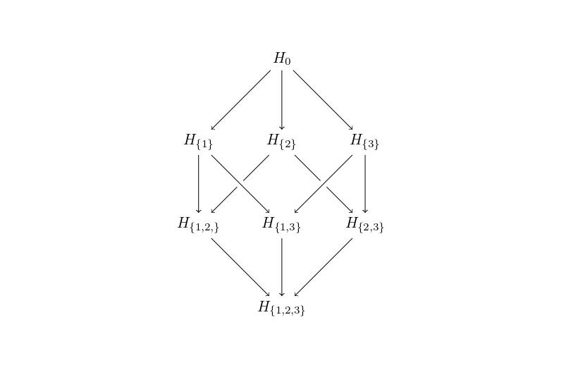 Figure 1
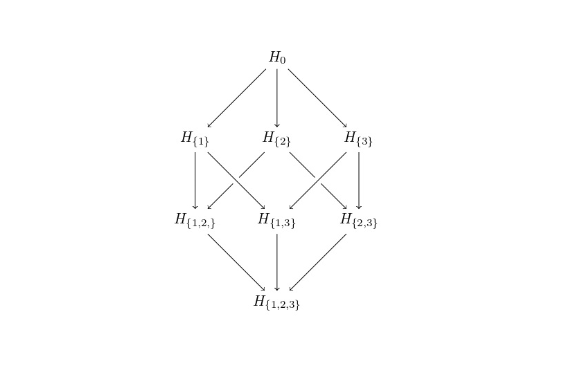 Figure 2