Cut-and-paste for impulsive gravitational waves with $\Lambda$: The geometric picture
Jiri Podolsky, Clemens S\"amann, Roland Steinbauer, Robert Svarc

TL;DR
This paper extends Penrose's geometric 'cut-and-paste' method to impulsive gravitational waves in (anti-)de Sitter spaces, providing a visualisation that clarifies their structure, junction conditions, and implications for the memory effect.
Contribution
It introduces a new geometric picture for impulsive waves in curved backgrounds, generalising Penrose's approach to non-zero cosmological constant scenarios.
Findings
Provides a visualisation of impulsive waves in (anti-)de Sitter space
Clarifies Penrose junction conditions in curved backgrounds
Enhances understanding of the memory effect in impulsive waves
Abstract
Impulsive gravitational waves in Minkowski space were introduced by Roger Penrose at the end of the 1960s, and have been widely studied over the decades. Here we focus on non-expanding waves which later have been generalised to impulses travelling in all constant-curvature backgrounds, that is also the (anti-)de Sitter universe. While Penrose's original construction was based on his vivid geometric `scissors-and-paste' approach in a flat background, until now a comparably powerful visualisation and understanding have been missing in the case. In this work we provide such a picture: The (anti-)de Sitter hyperboloid is cut along the null wave surface, and the `halves' are then re-attached with a suitable shift of their null generators across the wave surface. This special family of global null geodesics defines an appropriate comoving coordinate system, leading to the…
Click any figure to enlarge with its caption.
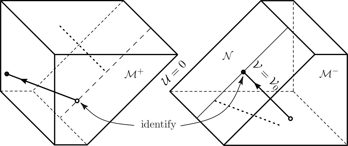 Figure 1
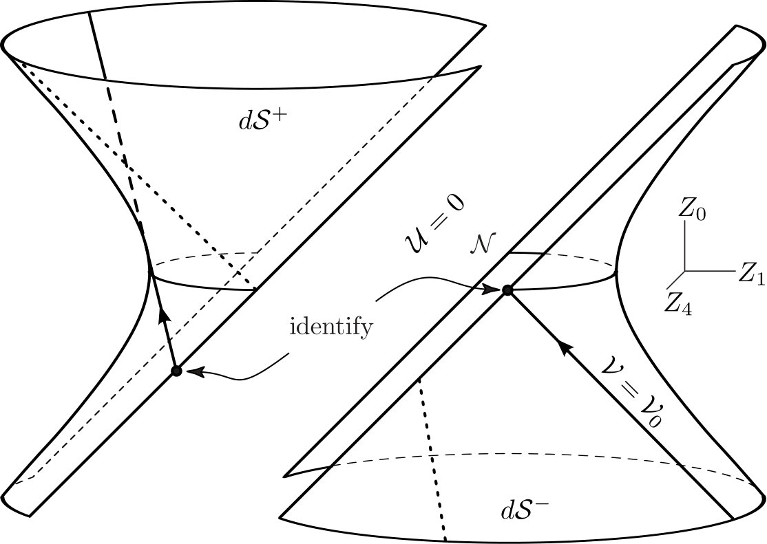 Figure 2
Peer Reviews
No public reviews on file for this paper yet. If you reviewed it on a platform where reviews are public (OpenReview, ICLR, NeurIPS, ICML), you can paste yours below so the community can read it here.
Videos
No videos yet. Explain this paper in a talk, walkthrough, or lecture? Add one.
Cut-and-paste for impulsive gravitational waves with :
The geometric picture
Jiří Podolský1, Clemens Sämann2, Roland Steinbauer2 and Robert Švarc1
1 Institute of Theoretical Physics,
Charles University, Faculty of Mathematics and Physics,
V Holešovičkách 2, 18000 Prague 8, Czech Republic.
2 Faculty of Mathematics, University of Vienna,
Oskar-Morgenstern-Platz 1, 1090 Vienna, Austria. [email protected]@[email protected]@mff.cuni.cz
Abstract
Impulsive gravitational waves in Minkowski space were introduced by Roger Penrose at the end of the 1960s, and have been widely studied over the decades. Here we focus on non-expanding waves which later have been generalised to impulses travelling in all constant-curvature backgrounds, that is also the (anti-)de Sitter universe. While Penrose’s original construction was based on his vivid geometric ‘scissors-and-paste’ approach in a flat background, until now a comparably powerful visualisation and understanding have been missing in the case. In this work we provide such a picture: The (anti-)de Sitter hyperboloid is cut along the null wave surface, and the ‘halves’ are then re-attached with a suitable shift of their null generators across the wave surface. This special family of global null geodesics defines an appropriate comoving coordinate system, leading to the continuous form of the metric. Moreover, it provides a complete understanding of the nature of the Penrose junction conditions and their specific form. These findings shed light on recent discussions of the memory effect in impulsive waves.
Keywords: impulsive gravitational waves, de Sitter space, anti-de Sitter space, cut-and-paste approach, Penrose junction conditions, null geodesics, memory effect
MSC2010: 83C15, 83C35, 83C10
PACS numbers: 04.20.Jb, 04.30.–w, 04.30.Nk
1 Introduction
Impulsive gravitational waves are theoretical models of short but violent bursts of gravitational radiation, which have been introduced by Roger Penrose in the late 1960s [19, p. 189ff], [18, p. 82ff]. Subsequently, in his seminal 1972 paper [20] he studied their geometry most explicitly using a vivid ‘scissors-and-paste’ approach111Nowadays more commonly referred to as cut-and-paste method. to construct impulsive pp-waves: Minkowski space is cut along a null hyperplane into two ‘halves’, which are subsequently re-attached with a warp, given by the so-called Penrose junction conditions, which guarantee that the field equations are satisfied everywhere, see Figure 1.
Penrose also presented these spacetimes in alternative forms using continuous or distributional metrics, for an overview see e.g. [7, Chapter 20], [2], [22]. Moreover, in a classical paper Peter Aichelburg and Roman Sexl [1] showed that certain impulsive pp-waves arise by boosting a Schwarzschild black hole to the speed of light. This AS-procedure has subsequently been applied to other geometries of the Kerr-Newman family, leading to more general impulses. The corresponding geometries have in turn been used as a playground for particle scattering at the Planck scales, see e.g. [15, 33].
In another landmark paper [10], Masahiro Hotta and Masahiro Tanaka in 1993 have managed to include a non-vanishing cosmological constant in the AS-procedure, thereby overcoming severe conceptional intricacies. They boosted the Schwarzschild-(anti-)de Sitter solution to the speed of light to obtain a non-expanding impulsive gravitational wave generated by null monopole particles propagating in (anti-)de Sitter space (abbreviated as (A)dS from now on). Their key-technique was to consider the boost in a convenient representation of (A)dS as hyperboloid in a -dim flat space.
In the late 1990s Jerry Griffiths together with the first author systematically studied the entire class of non-expanding impulsive gravitational waves travelling in (A)dS universe [23, 21, 25, 24], giving also an illustrative description of the geometry of the wave surfaces. These are spherical and hyperboloidal for and , respectively, see also [22, 26]. The explicit construction of the continuous form of the metric [25] was based on the use of conformally flat coordinates. In this approach the cosmological constant does not explicitly appear in the junction conditions, but an analogue of the vivid picture of Penrose’s cut-and-paste construction was not considered. In this work we present such a picture: The (A)dS hyperboloid is first cut along a null-hypersurface into two ‘halves’. These are then re-attached with the ‘dual’ null generators shifted along the generators of the wave surface by a suitable shift, which also changes their speeds. To obtain the details of this construction it is essential to understand the specific behaviour of the null geodesic generators of the (A)dS hyperboloid upon crossing the impulsive wave.
Here we draw on recent works [31, 29] which are in turn based on the analysis of [26]. The fact that it is essentially the behaviour of the null geodesics that determines the Penrose junction conditions, was first explicitly noted for in [34] and put to use in [11]. To emphasise this, we have included a null geodesic perpendicular to the wave surface in our Figure 1. It is not only shifted along the null generator of the wave surface but its speed also changes upon its interaction with the wave, see the ‘jump formulas’ e.g. [12, Thm. 3]. The paper [11] also provides a framework to address the Penrose junction conditions and the corresponding ‘discontinuous coordinate transformation’ in a mathematically rigorous way. The generalisation of the corresponding approach to the case of non-vanishing is now also possible. Its technical implementation is, however, deferred to a separate, more mathematically minded paper.
This letter is organized in the following way: In the next section we summarise the necessary prerequisites, introducing the various forms of the non-expanding impulsive wave metrics, thereby fixing our notations. In the main technical section 3 we study in detail the interaction of the null geodesic generators of the (A)dS hyperboloid with the wave impulse. Then we present our main result, which is the geometric account on the Penrose junction conditions in section 4. Finally, we discuss the way in which our analysis leads to a mathematically watertight treatment of the ‘discontinuous coordinate transformation’ relating the (-dim) continuous and the distributional forms of this large class of impulsive wave metrics to one another.
2 Non-expanding impulsive waves with
To begin, we give a brief account on the various construction methods of non-expanding impulsive gravitational waves with following [7, Chapter 20]. We start with the conformally flat form of the constant-curvature (i.e., Minkowski and (A)dS) backgrounds
[TABLE]
where are the usual null and the usual complex spatial coordinates. Next we apply the coordinate transformation separately for negative and positive values of ,
[TABLE]
where is any real-valued function. This leads to the continuous form of the metric [21, 25]
[TABLE]
where222This choice of sign of is in accordance with [26, 31, 29], which are our main points of reference, but different from e.g. [27]. and for and for is the kink function. Hence the metric (3) is of local Lipschitz regularity in which is beyond the reach of classical smooth Lorentzian geometry. The latter reaches down to — at least as far as convexity and causality are concerned [16, 13, 14, 5]. However, the Lipschitz property is decisive since it prevents the most dramatic downfalls in causality theory which are known to occur for Hölder continuous metrics [9, 3, 30, 6, 17]. More specifically, in the context of the initial value problem for the geodesic equation, the Lipschitz property guarantees the existence of solutions [35] which, due to the special geometry of the models at hand, are even (globally) unique [27].
The corresponding distributional metric for non-expanding impulsive waves in any constant-curvature background has the form [28]
[TABLE]
where is the Dirac-measure and is a real-valued function. Actually, it can formally be derived from (3) by rewriting (2) in the unified form of a ‘discontinuous coordinate transformation’ using the Heaviside function as
[TABLE]
with the specification
[TABLE]
and keeping all distributional terms. Although the metric (4) possesses a distributional coefficient and consequently lies beyond Geroch-Traschen’s ‘maximal sensible class’ of metrics [4], by their simple geometric structure the (distributional) curvature can be computed unambiguously leading to an impulsive component .
The Penrose junction conditions can now be explicitly obtained from the transformation (2). More precisely, defining and we can read off the following relation by taking the limits and in (2)
[TABLE]
While the ‘discontinuous transformation’ (2) thus provides a clear geometric picture, by its lack of smoothness, it is mathematically not meaningful. Nevertheless, in the special case of pp-waves (for ), nonlinear distributional geometry [8, Ch. 3] was invoked to provide a rigorous mathematical interpretation of (2) as a ‘generalised diffeomorphism’ [12]. There the key step was a detailed study of the geodesics in the distributional form of the metric. This study has recently been generalized in [31, 29] to the case, and we will employ these results as well as those of [26] to give a clear geometric interpretation of the transformation (2) in the general case.
These works all use a convenient -dim formalism, and here we will also employ it to explicitly study the null geodesic generators of the (A)dS hyperboloid and their interaction with the impulsive wave. Specifically, we consider the -dim impulsive pp-wave manifold
[TABLE]
with the constraint
[TABLE]
and the parameters given by and . Using the metric (8) with (9) we can easily see the geometry of the impulsive wave spacetime: The impulse is located on the null hypersurface , which is
[TABLE]
corresponding to a non-expanding 2-sphere for and a hyperboloidal 2-surface for . The manifold (8), (9) is related to the -dim form (4) via
[TABLE]
where we use the abbreviation and the associated real coordinates
[TABLE]
as well as the relation
[TABLE]
3 Explicit null geodesics
The key point is to analyse in detail the null geodesics in the impulsive wave spacetimes at hand. Since we ultimately are interested in understanding the transformation (2) relating the two -dim forms (3), (4) of the metric to one another, we start with the geodesics of (4) ‘before’ the impulse, i.e., for . Then we will turn to the -dim representation (8), (9) for two distinct reasons: We have to base our approach on the rigorous results on such geodesics in this representation [26, 31, 29] rather than on the analysis using the -dim approach given in [27], which uses the continuous form of the metric (3). Indeed, in the latter the transformation (2) was explicitly used to derive the form of the geodesics and hence such an approach would lead to a circular argument. Second, the -dim approach leads to a very vivid picture paralleling the one given in Figure 1.
3.1 Background null geodesics in the -dim form (4)
We first explicitly determine a convenient family of null geodesics of the (A)dS background (1), since away from the impulse they will coincide with null geodesics in the impulsive wave (4). To be consistent with the standard case, we choose the following family of geodesics in flat space using the coordinates ,
[TABLE]
These are parametrised by the three real constants , , and . They give the position of the geodesic at the parameter value , which, in the later context, will be the instant when the wave impulse is crossed. Next we apply the conformal transformation to explicitly derive the corresponding null geodesics of the (A)dS background (1). To obtain an affine parameter , we use the relation
[TABLE]
with , and
[TABLE]
where we have defined
[TABLE]
To explicitly integrate (15), we distinguish two cases depending on the value of (which is proportional to ):
- (1)
: Here we trivially obtain , i.e., , and it is natural to set to have iff . The ansatz (14) thus leads to the null geodesics
[TABLE] 2. (2)
: In this case , i.e., , and we again impose the condition to fix the parameter . Thus , which finally implies
[TABLE]
3.2 Background null geodesics in the -dim form (8),
(9)
Next we connect the family of null geodesics (18) and (19) to those of the -dim parametrisation using the coordinates of the (A)dS universe. In general, they can be written as [26, eq. (29)]
[TABLE]
The integration constants are constrained by condition (9), its derivative with respect to the parameter , and the normalization of the -velocity, that is explicitly by
[TABLE]
Using the simple transformation (11), the -dim background null geodesics corresponding to (18) and (19) are
[TABLE]
respectively. We immediately observe the following:
- (1)
The constant in the second expression can be set to zero, , to formally obtain the first one. We can thus continue only with the more general second expression of the -dim geodesics. 2. (2)
The initial value of the coordinate is zero, i.e., . 3. (3)
W.l.o.g. we may set corresponding to , and we will do so in the following.
Consequently, we obtain the following explicit -dim representation of the null generators
[TABLE]
parametrised by the -dim initial data . Notice from the first line that, interestingly,
[TABLE]
Finally, by comparing (20) with (25) we can now identify the complete set of -dim data in terms of the -dim data via
[TABLE]
with , given by (17).
3.3 Global null geodesics in the -dim impulsive
The global geodesics in the -dim distributional representation of non-expanding impulsive gravitational waves were first derived in [26] using a formal approach. These results have been recently confirmed by a careful regularisation analysis in the following sense [31]: The geodesics in a general regularisation of (8), (9), where the Dirac-delta is replaced by a generic mollifier, converge to the distributional geodesics of [26]. For our purpose it suffices to deal with the global null geodesics which have and . In the coordinates where , they take the explicit form [31, Sec. 5]
[TABLE]
with , and ()
[TABLE]
Here and denote the values of and its respective spatial derivatives at the instant of interaction of the geodesic with the wave impulse, i.e., at the parameter value , see (26). Also, in the term summation over is understood.
In this general family of global null geodesics, we can identify those which coincide with the special family of background null geodesics (25) in front of the impulse by simply substituting the constants (27) into (3.3).
3.4 Global null geodesics in the -dim impulsive
metric (4)
Finally, we rewrite these global null geodesics (with the particular choice of initial data (18), (19)) in the -dim metric form (4). To this end, we transform (28) with (27) substituted into (3.3) using the inverse of (11),
[TABLE]
Moreover, we have to rewrite the derivatives of the function on the impulse using and its derivatives, see (13), namely333Here we use the relations and .
[TABLE]
where . A lengthy calculation leads to
[TABLE]
where
[TABLE]
In addition, using (27), (28), and (32), the conformal factor in (30) takes the form
[TABLE]
Finally, by combining (28) with (32) and (30), the specific class of global null geodesics corresponding to the solutions (18), (19) in front of the impulse, take the following form in the -dim ‘distributional’ coordinates
[TABLE]
Here, we have denoted the dependence on the initial data explicitly, and we have used the abbreviation
[TABLE]
Recall also that the constants , are given by (17).
At this point, we infer from the first line in (38) that
[TABLE]
Observe that (since , and ) and have the same sign, and vanish simultaneously on the impulse. This implies , and together with (40) we obtain
[TABLE]
This allows us to finally express our special family of null geodesics (38) in the simple explicit form
[TABLE]
In the following section, we will use this final result to clarify the geometric nature of the comoving ‘continuous’ coordinate system and the related Penrose junction conditions for the entire class of non-expanding impulsive gravitational waves in (A)dS backgrounds.
4 Cut-and-paste with
Let us now discuss the results derived in the above section. Most importantly, the final formula (45) tells us that the discontinuous transformation (2) is closely related to special geodesics in the distributional spacetime (4), namely the null geodesic generators of the (A)dS hyperboloid. Indeed, the explicit form (45) of these geodesics, which are jumping in the -coordinate, and suffer a kink in as well as in the transverse spatial coordinates , matches exactly the transformation (2).
To be more precise, we can employ (45) to transform the coordinates in which the metric is continuous (cf. (3)) to the coordinates in which the metric is distributional (cf. (4)) via
[TABLE]
with the standard relations and . Observe also from (6) that
[TABLE]
and similarly for the spatial derivatives. Hence (46) fully coincides with (2), and we have thus derived the ‘discontinuous transformation’ from a special family of unique global null geodesics of the impulsive wave in the distributional form, obtained previously by a general regularisation procedure in [31].
Moreover, we explicitly see that the transformation (2) respectively (46) turns the special geodesics (45) into coordinate lines, hence the coordinates are comoving with the corresponding null particles. In fact, that is the way how the distributional metric (4) in coordinates is transformed to the much more regular, (locally Lipschitz) continuous metric (3) in the coordinates . This generalises (and is in perfect agreement with) the flat case , in which the Rosen coordinates for pp-waves are again comoving, cf. [34, 12].
This insight can now be put to use to arrive at a vivid picture illustrating the cut-and-paste approach in the -case, see Figure 2. Here we exclusively concentrate on the de Sitter case, the anti-de Sitter case being analogous.
The de Sitter hyperboloid is cut into two ‘halves’ and along the non-expanding spherical impulsive surface (for its geometry see [23, Fig. 3]). Then the two parts are re-attached in the following specific way: The null geodesic generators of the two halves are joined according to (45), or (28) with (27) substituted into (3.3) in the -dim picture, depending on . We will refer to this -dim picture in the remainder of this discussion, since it is more directly related to Figure 2. More precisely, the generators (25) approaching the impulse at from are shifted from the value in to the value in due to the interaction with the wave. They are also tilted (deflected) by the impulse according to , cf. (28), which is precisely the amount needed to turn them into the generators of starting at .
Note, however, the following subtlety: In Figure 2 the - and -directions are suppressed, so that the two families of null generators plotted in each ‘half’ (i.e., those whose only spatial movement is in the -direction) need not in general be the ones that get matched. The reason is that the impulse induces a motion in the - and -directions as is evident from the -term in the spatial part of (28) and the nontrivial constants in (3.3)444Observe that this effect already occurs in the flat case, see Figure 1.. However, if we specialise to waves with , the depicted generators which satisfy implying , are precisely the ones shown in Figure 2. Indeed, in this case we have (cf. (27), (3.3)) and the interaction with such an impulse does not induce any motion in the -directions since by (28) for all . So the null generators of and depicted in Figure 2 are indeed matched to one another.
This explicit visualization thus provides us with a clear geometric insight. It yields a deeper understanding of the various construction methods of impulsive gravitational waves in de Sitter and anti-de Sitter universes. Moreover, it gives a natural explanation on their mutual unambiguous relations, because the key elements of the overall geometric picture — the null generators — are globally unique.
5 Discussion and outlook
We have given a vivid interpretation of the Penrose junction conditions and the corresponding ‘discontinuous coordinate transformation’ which relates the continuous and distributional metric forms of the entire class of non-expanding impulsive gravitational waves travelling in an (A)dS background. It is based on an explicit study of the null geodesics in the distributional -dim form of the metric, which have been derived via a general regularisation procedure in [31]: The (A)dS hyperboloid is cut into two ‘halves’ along the null wave surface , which are then re-attached in such a way that the null geodesic generators of both ‘halves’ are matched with a shift in the -direction. The ‘discontinuous coordinate transformation’ which turns these broken and refracted null generators into coordinate lines also transforms the distributional form of the metric into the continuous one.
In the case this notorious transformation has been treated in a mathematically rigorous way. In [12] it was shown to be connected to a ‘generalised diffeomorphism’ in the framework of nonlinear distributional geometry [8, Ch. 3]. The geometric insight provided by the present work paves the way to a generalisation of this approach to the case of nonvanishing . Indeed, building on the fully nonlinear distributional analysis of the geodesics in the -dim picture [29] the transformation (46) can now be shown to be a (distributional) limit of a ‘generalised diffeomorphism’, which is built up from a regularised version of the geodesics (28). The details of this account will be studied in a separate, more mathematically oriented paper [32].
Finally, our current findings have some consequences for studying the wave memory effect in impulsive spacetimes. In particular, the geometric picture established above makes it obvious that the arguments recently put forward in [36] simply extend to (A)dS backgrounds: The interaction of test particles with the wave impulse can be seen most explicitly and the difference of their positions and velocities before and after the wave has passed can simply be read off from the matching conditions already derived in [27, Sec. 4]. (In particular, there is no need to involve the symmetries of the (A)dS background.) A comprehensive study of the memory effect in impulsive wave spacetimes is, however, subject to current research and will be detailed elsewhere.
Acknowledgement
This work was supported by project P28770 of the Austrian Science Fund FWF, the WTZ-grant CZ12/2018 of OeAD/the Czech-Austrian MOBILITY grant 8J18AT02, and the Czech Science Foundation Grant No. GAČR 19-01850S.
The reference list from the paper itself. Each links out to its DOI / PubMed record.
- 1[1] P. C. Aichelburg and R. U. Sexl. On the gravitational field of a massless particle. Gen. Rel. Grav. , 2:303–312, 1971.
- 2[2] C. Barrabès and P. A. Hogan. Singular null hypersurfaces in general relativity . World Scientific Publishing Co., Inc., River Edge, NJ, 2003.
- 3[3] P. T. Chruściel and J. D. E. Grant. On Lorentzian causality with continuous metrics. Class. Quant. Grav. , 29(14):145001, 32, 2012.
- 4[4] R. Geroch and J. Traschen. Strings and other distributional sources in general relativity. Phys. Rev. D , 36(4):1017–1031, 1987.
- 5[5] M. Graf, J. D. E. Grant, M. Kunzinger, and R. Steinbauer. The Hawking-Penrose singularity theorem for C 1 , 1 superscript 𝐶 1 1 C^{1,1} -Lorentzian metrics. Comm. Math. Phys. , 360(3):1009–1042, 2018.
- 6[6] J. D. E. Grant, M. Kunzinger, C. Sämann, and R. Steinbauer. The future is not always open. preprint, ar Xiv:1901.07996 [math.DG] , 2019.
- 7[7] J. B. Griffiths and J. Podolský. Exact Space-Times in Einstein’s General Relativity . Cambridge University Press, Cambridge, 2009.
- 8[8] M. Grosser, M. Kunzinger, M. Oberguggenberger, and R. Steinbauer. Geometric theory of generalized functions with applications to general relativity , volume 537 of Mathematics and its Applications . Kluwer Academic Publishers, Dordrecht, 2001.