A learning-enhanced projection method for solving convex feasibility problems
Janosch Rieger

TL;DR
This paper introduces a generalized projection method for convex feasibility problems that learns from past projection steps to improve decision-making, with proven convergence and initial numerical results.
Contribution
It presents a novel learning-enhanced projection algorithm that adapts based on previous steps, extending traditional cyclic projection methods.
Findings
Proven convergence of the proposed algorithm.
Initial numerical experiments demonstrate its effectiveness.
The method adapts projections based on learned geometric information.
Abstract
We propose a generalization of the method of cyclic projections, which uses the lengths of projection steps carried out in the past to learn about the geometry of the problem and decides on this basis which projections to carry out in the future. We prove the convergence of this algorithm and illustrate its behavior in a first numerical study.
Click any figure to enlarge with its caption.
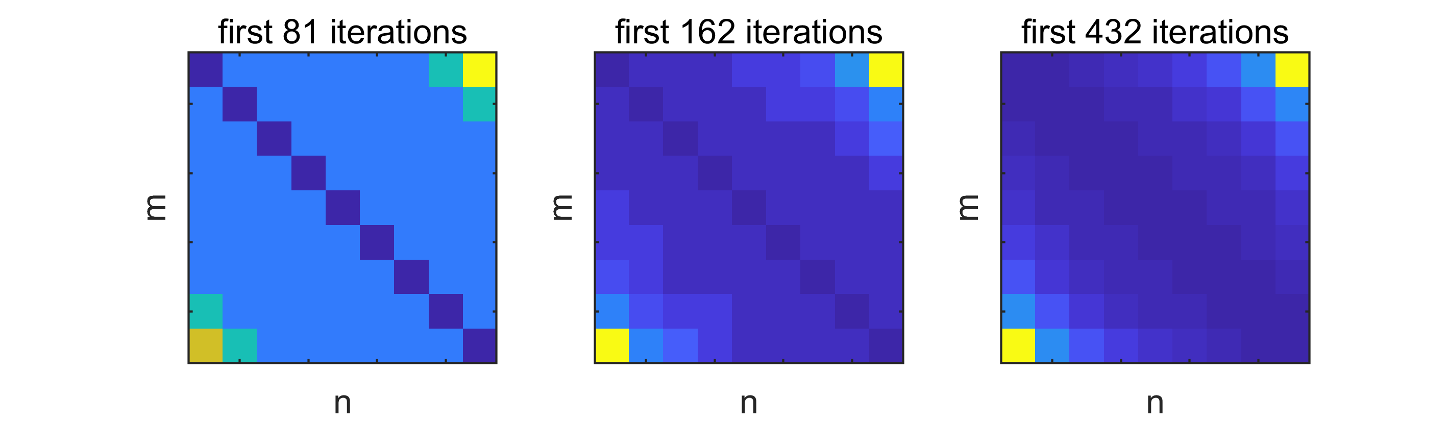 Figure 1
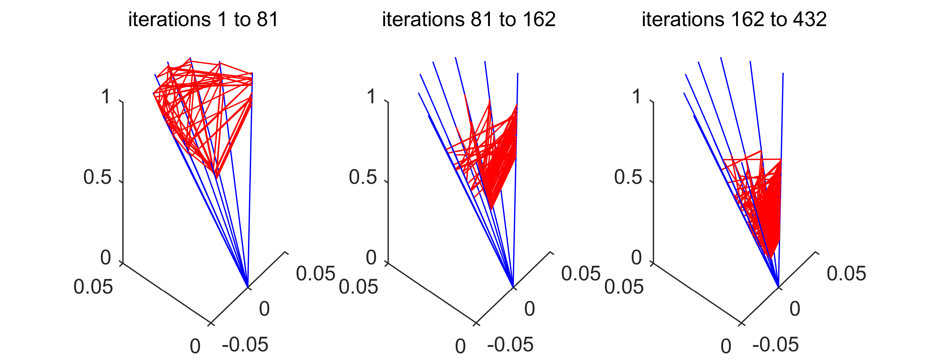 Figure 2
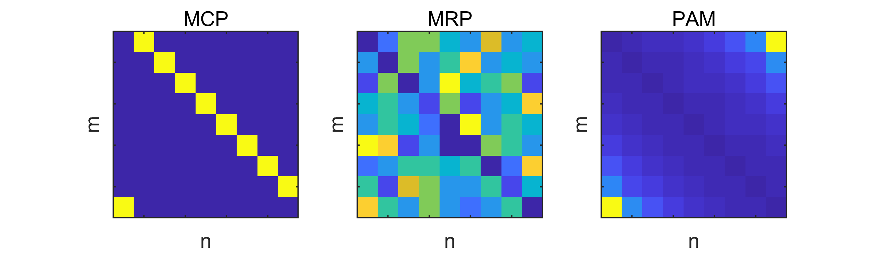 Figure 3
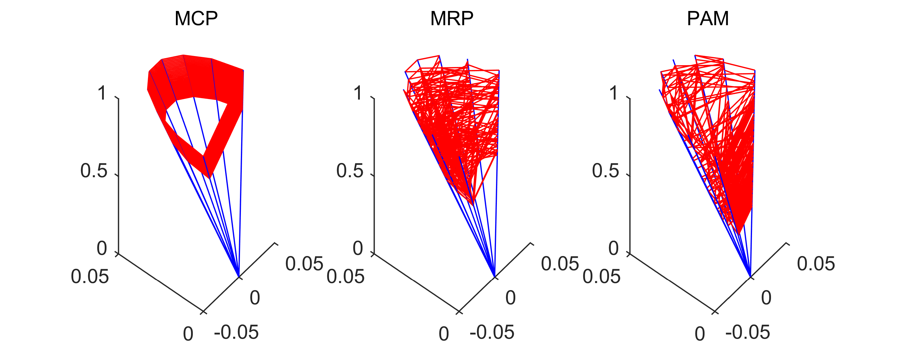 Figure 4
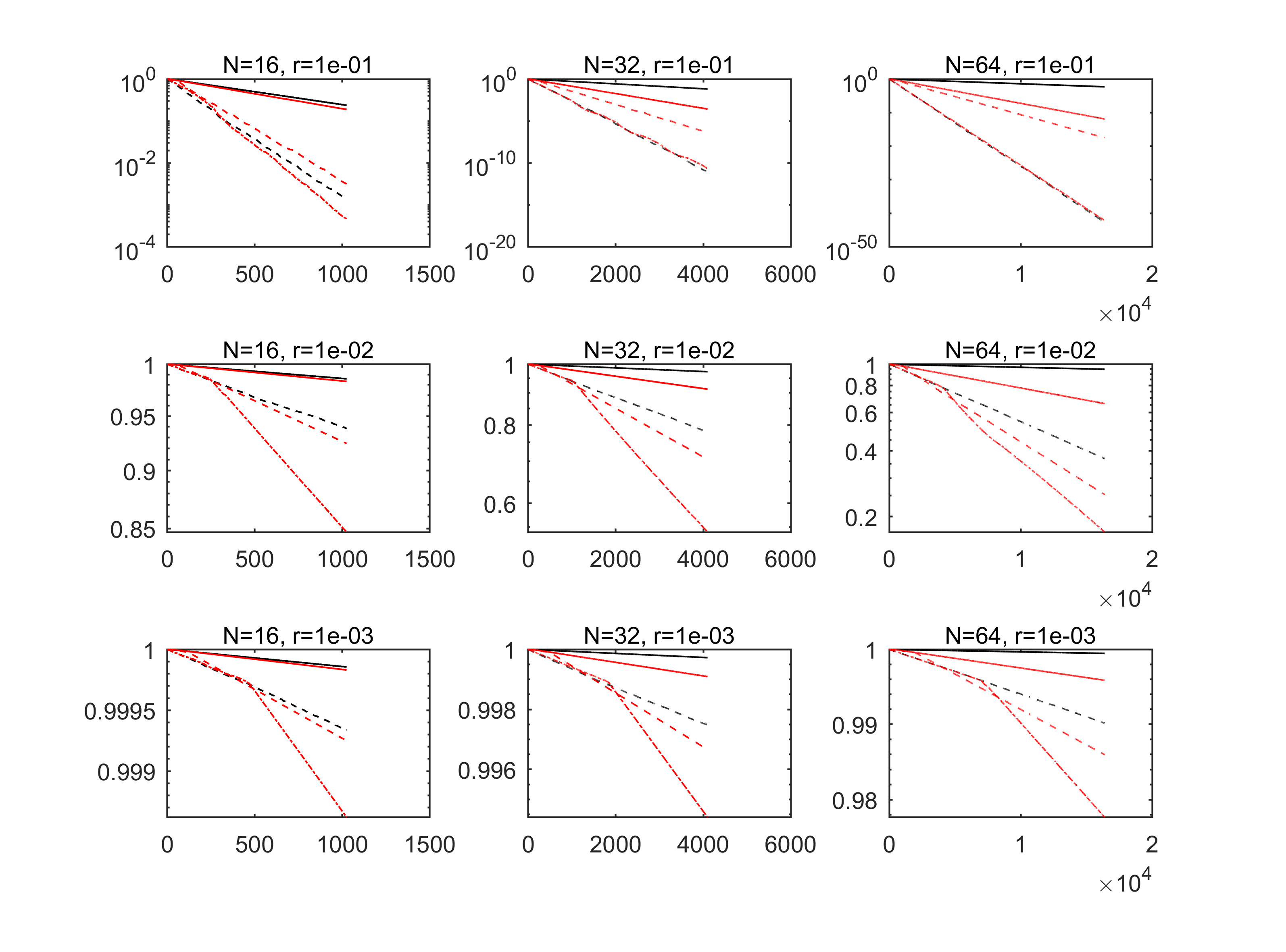 Figure 5
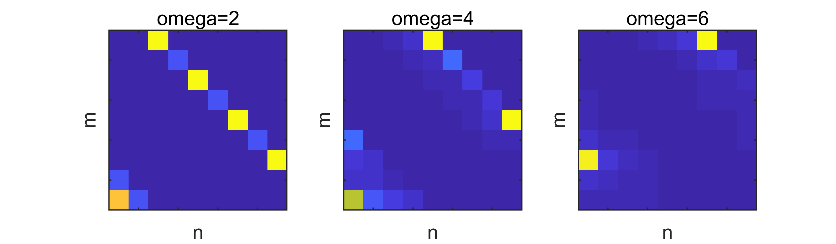 Figure 6
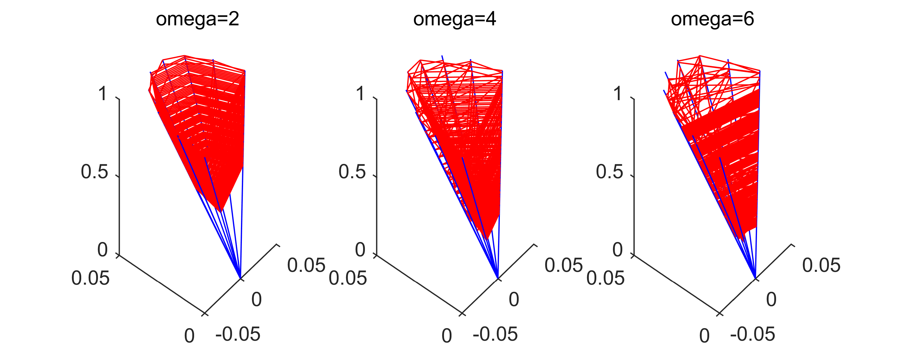 Figure 7
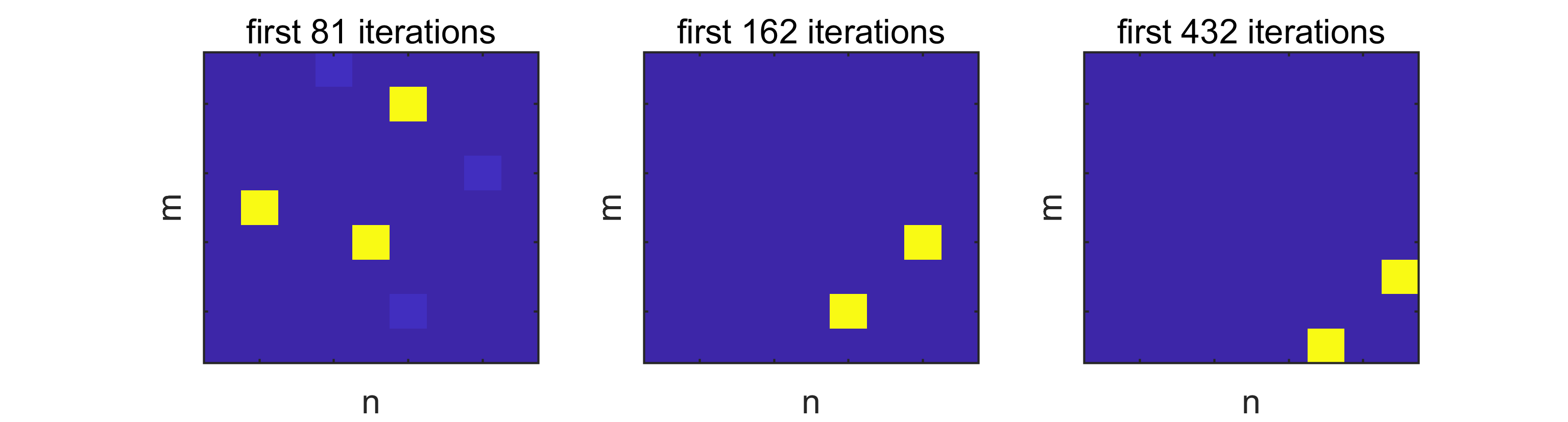 Figure 8
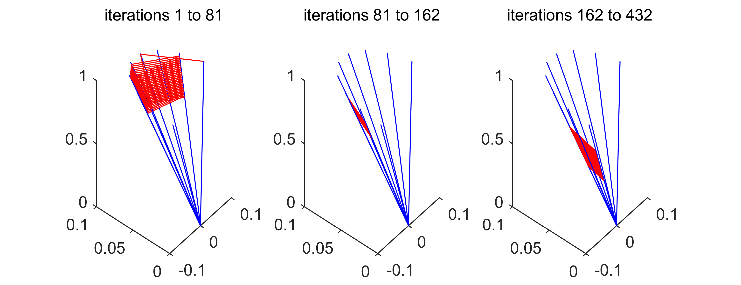 Figure 9
Peer Reviews
No public reviews on file for this paper yet. If you reviewed it on a platform where reviews are public (OpenReview, ICLR, NeurIPS, ICML), you can paste yours below so the community can read it here.
Videos
No videos yet. Explain this paper in a talk, walkthrough, or lecture? Add one.
A learning-enhanced projection method for solving convex feasibility
problems
Janosch Rieger
Abstract
We propose a generalization of the method of cyclic projections, which uses the lengths of projection steps carried out in the past to learn about the geometry of the problem and decides on this basis which projections to carry out in the future. We prove the convergence of this algorithm and illustrate its behavior in a first numerical study.
MSC Codes: 65H20, 52B55, 37B20, 90C59
Keywords: Method of cyclic projections, acceleration of convergence, convex feasibility problem
1 Introduction
The method of cyclic projections, originally proposed in [7], is an established numerical algorithm, which computes a point in the intersection of finitely many closed convex subsets of a Hilbert space when this intersection is nonempty. A broad overview over convergence properties of this method as well as the underlying theory is given in [3], [4], [10] and the references therein.
Estimates for the speed of convergence of the method of cyclic projections are well-known in the case when the sets are affine linear subspaces. For this situation, accelerated variants of the original scheme, which are often based on line-search ideas, have been developed, see e.g. [5] and [13]. Recently, a first result on the speed of convergence of the method of cyclic projections has been given in the case of semi-algebraic sets, see [6]. In general, however, the method can be arbitrarily slow, see [12] for a pathological example.
When the sets are affine linear subspaces with codimension 1, the method of cyclic projections reduces to the Kaczmarz method, see [16], which has gained popularity in the context of very large, but sparse consistent linear systems, see [8]. A probabilistic version of this algorithm, which converges exponentially in expectation, has been introduced in [17], and an accelerated version of this method has been proposed in [2]. The Kaczmarz method is frequently used in medical imaging, see [15], where block and column action strategies have become a topic of active research interest [1] and [11].
The numerical method presented in this paper is supposed to accelerate the method of cyclic projections in settings where the above-mentioned refined algorithms for subspaces are not applicable. The guiding idea behind the method is to gather as much information on the relative geometry of the closed convex sets from the lengths of the projection steps carried out in the past. This is motivated by the convergence proof in [7], which reveals that the performance of the algorithm is in worst case determined by the lengths of the projection steps carried out.
We prove that our method converges, using techniques which are common in the dynamical systems community. The main challenge is to guarantee convergence for a reasonably broad class of strategies our basic algorithm can be equipped with. As it seems very hard to quantify a speed of convergence even in the subspace case, we provide several numerical studies performed on a toy example, which provide some insight as to why and how our method can outperform the standard methods of cyclic and random projections.
2 The algorithm
Given closed convex sets with , we wish to find a point . We first present two common projection algorithms for solving this problem in Section 2.1. Then we propose a new projection algorithm in Section 2.2, which learns the geometry of the problem to some extent from the lengths of the projection steps carried out in the past and uses this knowledge to select favourable projections in the future.
The notation used in this paper is mostly standard. Given a point and a closed convex set , it is well-known that the projection
[TABLE]
of to exists and is a unique point.
By we denote a permutation of the numbers which is sampled uniformly from the set of all such permutations, and by , we denote a uniform random sample from an index set .
2.1 The benchmark: MCP and MRP
The now classical method of cyclic projections, which was originally published in [7], approximates a point by iteratively projecting to the sets in a cyclic fashion, see Algorithm 1.
Algorithm 1 may converge very slowly when many of the projection steps are small. This behavior may originate from an unfavorable ordering of the sets , which can be helped by randomly shuffling the order of the sets in every cycle, see Algorithm 2.
The random Kaczmarz method proposed in [17] is a prominent variant of Algorithm 2 in the framework of row-action methods for solving linear systems, which is known to converge in expectation. Since MRP slightly outperformed the random Kaczmarz method in all examples we have studied, we use MRP as the benchmark for randomized algorithms.
2.2 A projection algorithm with learning ability
The idea behind Algorithm 3 (PAM) is to keep a record of the lengths of projection steps performed in the past and to give preference to operations that have lead to large projection steps. This enables our algorithm to learn to some extent the geometry of the problem with manageable additional computational cost.
From a formalistic point of view, our approach resembles to some extent the techniques of loping and flagging introduced in [11] in the setting of row-action methods. These techniques suppress the effect of noise in the data on MCP by ignoring projections which had very small residuals in previous cycles. From a phenomenological perspective, however, these modifications of MCP do not have much in common with PAM.
In the following, we give an intuitive description how some of the individual components interact in Algorithm 3. They will be treated with proper mathematical rigour in the next section.
- i)
The sequence of matrices records – up to the impact of the function – the length of the -th projection step from set to in the component .
- ii)
The input has three distinct effects.
- a)
If , a transition from to will not occur during the entire runtime of the algorithm, see Lemma 5. Thus, by choosing a sparse as in Example 2(i), one can limit the amount of information that needs to be stored and processed at runtime. For a graphic illustration, see Example 12, and for the impact on performance in the context of a toy model, see Example 13.
- b)
The choice of can incorporate a priori knowledge: The more likely a transition from to is to be beneficial, the larger the entry should be chosen, see Example 2(ii).
- c)
If the entries of are small relative to the first several lengths of steps to be carried out, the algorithm will not perform well in an initial stage, see Example 11(ii). If they are larger, the algorithm will initially behave like MRP, see Example 11(i).
- iii)
The function modifies the step length before it is recorded in the matrix .
- a)
It ensures that only strictly positive values are written into .
- b)
It determines at what level of overall performance a transition from to will get reactivated after it generated a short step.
Finally, we would like to mention that we represent the recorded step-lengths in a matrix to keep the notation manageable. Depending on the size of the problem, the sparsity pattern of and the policy , it can be beneficial to use a different data structure – such as one red-black tree per set – to store and search this data with moderate on-cost compared to MCP and MRP.
3 Admissible input
For Algorithm 3 to converge, we require the inputs to have certain properties. The matrix is required to be irreducible in the following sense.
Definition 1** (admissible matrix).**
A matrix is called admissible if it satisfies
- i)
* for all , and*
- ii)
for any indices with , there exist some and indices such that
[TABLE]
We give a few examples how the matrix can be chosen.
Example 2** (some admissible matrices).**
For a good performance of Algorithm 3, it is helpful to multiply the matrices proposed below with a positive scalar to ensure that their respective nonzero entries are – at least on average and for small – similar to or larger than the length of the -th projection step from set to .
i) To limit the effective size of the matrices , one can choose to be a sparse matrix such as the banded matrices given by
[TABLE]
and given by
[TABLE]
with some with .
ii) In scenarios, where the concept of an angle makes sense, it is reasonable to work with a matrix given by
[TABLE]
to introduce a bias in favour of transitions with large angles, which are more likely to result in large step-lengths.
It is easy to check that the above matrices are admissible. Please note that MCP is a special case of Algorithm 3, which can be realized by choosing to be the matrix with .
The function is required to be strictly positive on all meaningful input, and it must ensure a certain decay of the entries of .
Definition 3** (admissible policies).**
A function
[TABLE]
is called an admissible policy if there exists such that
- i)
* holds for all and satisfying , and*
- ii)
* for all and .*
We propose some particular policies .
Example 4** (some admissible policies).**
It is easy to check that both policies proposed below are indeed admissible for every .
i) The function
[TABLE]
ensures that the number which is written into the distance matrix in line 7 of Algorithm 3 is at least times the minimal previously recorded step-length from to another .
ii) The function
[TABLE]
ensures that the number which is written into in line 7 of Algorithm 3 is at least times the average of the previously recorded step-lengths from to another .
Note that the value of the minimal nonzero entry in a row as well as the average of the nonzero entries in a row can be updated with negligible computational cost in every step.
The proof of the following statement is elementary.
Lemma 5** (preservation of sparsity pattern).**
Let both and be admissible, and let be the matrices generated by Algorithm 3 with arbitrary initial value . Then for any and , we have
[TABLE]
and, in particular, the matrices are admissible for all .
4 Convergence analysis
We first prove a general principle for projection algorithms in Section 4.1. Then we show in Section 4.2 that Algorithm 3 satisfies the assumptions of this statement.
4.1 Recurrence implies convergence
We restate a slightly modified version of Corollaries 1 and 2 from [7].
Lemma 6** (projections reduce error).**
Let be closed convex sets and , and let the sequences and satisfy
[TABLE]
Then we have
[TABLE]
Now we show that every projection algorithm, which projects to every set infinitely often, generates a sequence that converges to a point in . Related results are known in the community working on firmly nonexpansive operators, see Theorem 4.1 from [9]. We include an explicit statement of this fact and an elementary proof to keep the paper self-contained.
Proposition 7** (recurrence implies convergence).**
Let be closed convex sets with , and let and be sequences which satisfy
[TABLE]
as well as the recurrence condition
[TABLE]
Then there exists such that .
Proof.
Because of statement (2) of Lemma 6, there exist a subsequence of and such that
[TABLE]
Clearly, there exist and a subsequence of the sequence with
[TABLE]
Since is closed, we have . We partition into
[TABLE]
By the above, we have . Assume that . By induction, using statement (3), we can construct sequences and given by and the iteration
[TABLE]
for . In particular, we have
[TABLE]
Since is finite, there exists such that
[TABLE]
By construction of the sequence , there exists such that
[TABLE]
Applying statement (2) of Lemma 6 with and the system of sets , and using the construction of the sequence , we obtain
[TABLE]
On the other hand, we have for all , so
[TABLE]
Now let and use statement (5) and statement (1) from Lemma 6 multiple times to obtain
[TABLE]
which is a contradiction. Hence , and . Now statements (4) and statement (2) of Lemma 6 with imply , as desired. ∎
4.2 Convergence of PAM
We check that Algorithm 3 satisfies the assumptions of Proposition 7, whenever the matrix and the policy are admissible.
Proposition 8** (PAM is recurrent).**
Let be closed convex sets which satisfy , and let the matrix and the policy be admissible. Then for any initial point , the sequences and generated by Algorithm 3 satisfy
[TABLE]
Proof.
Let . Applying inequality (1) from Lemma 6 multiple times yields
[TABLE]
which forces
[TABLE]
Let us denote
[TABLE]
Obviously, we have . Let , and let be the maximal strictly increasing sequence with for all . Let . By statement (8), there exists such that
[TABLE]
Because of line 6 of Algorithm 3 and since is admissible with a decay rate , we have
[TABLE]
Now let be such that . We wish to show that
[TABLE]
To this end, we introduce the quantity
[TABLE]
and prove the statement
[TABLE]
by induction. Statement (11) is trivial for . Assume that statement (11) holds for some . If , then statement (9) implies that , and that the induction hypothesis (11) holds for . If , then line 3 of Algorithm 3 selects an index
[TABLE]
that satisfies
[TABLE]
By line 6 of Algorithm 3 and by statemenr (9), we have
[TABLE]
By construction of the sequence , it follows that
[TABLE]
so , and statement (11) holds for . This completes the induction, and statement (10) is verified, because . Since , statements (9) and (10) imply that there exists such that for all . Since and were arbitrary, we have shown that
[TABLE]
In view of Lemma 5, this implies
[TABLE]
Since satisfies part ii) of Definition 1, a simple recursion on statement (13) yields , which is statement (7). Consequently, statement (12) implies (6). ∎
Now we summarize the above in the main theoretical result of this paper.
Theorem 9** (convergence of PAM).**
Let be closed convex sets which satisfy , and let the matrix and the policy be admissible. Then there exists such that the sequence generated by Algorithm 3 satisfies
[TABLE]
Proof.
Proposition 8 verifies that Algorithm 3 satisfies the assumptions of Proposition 7, so PAM is indeed convergent. ∎
5 An instructive toy example
We explore the performance of PAM with different matrices and policies in a very simple toy example, and compare its behavior with MCP and MRP. We are fully aware that this example has many unrealistic features, but it allows us to illustrate key features of our algorithm in a nice graphic way. To keep things simple, we measure the computational cost of all three algorithms in the number of iterations, which is the number of projection steps carried out.
Throughout this section, we consider the one-dimensional subspaces
[TABLE]
with , and the initial point . For aesthetical reasons, we choose and in most illustrations.
Let us first compare MCP, MRP and PAM without going into too much technical detail.
Example 10** (benchmark versus PAM).**
In Figure 1, we see at a glance how the strategies behind MCP, MRP and PAM impact their behavior and performance when applied to the toy model. The fixed order of projections in MCP can result in significant underperformance, while the random order of the projections in MRP guarantees that the average of the achievable progress is realized.
This motivates us to try and outperform the average by assigning a high probability to transitions, which performed better than average in previous iterations, in the new method PAM. The toy problem suggests that this is not a bad idea, when the matrix and the policy are chosen well for the problem at hand. For this showcase, we used and as in Example 11a), and carried out 315 iterations with each method.
In Example 11, we examine how a good performance of PAM can be achieved by a proper scaling of the initial matrix . Please note that the intention of this example is not to discuss the size of numerical errors, but rather the qualitative behavior of PAM. The matrices and the iteration numbers are chosen in such a way that these characteristics become clearly visible.
Example 11** (scaling ).**
i) In Figure 2, we apply PAM with , and initial matrix given by
[TABLE]
While the entries of the matrix are large compared to the actual step-sizes of the algorithm, we see a more or less uniform sampling of the transitions, similar to the behavior of the superior benchmark method MRP. Once the sizes of the entries of the matrix are similar to the sizes of the steps carried out, PAM has learned the geometry of the problem and focusses with high probability on profitable transitions, which allows it to outperform MRP.
ii) In Figure 3, we apply PAM with , and initial matrix given by
[TABLE]
so the entries of the matrices underestimate the actual step-sizes in the initial phase of the algorithm. This leads to unpredictable qualitative behaviour of PAM and incomplete exploration of the admissible transitions, and in many cases to an underperformance relative to MRP. Once the sizes of the entries of the matrix are similar to the sizes of the steps carried out, the qualitative behavior will be as in part i) above.
The effect of choosing a sparse is not surprising.
Example 12** (sparse ).**
We apply PAM to the model problem with , and the matrix from Example 2 with parameters , and obtain the results shown in Figure 4 after 432 iterations. Note that the matrix overestimates the first step-lengths of the algorithm and therefore needs no scaling.
The algorithm behaves exactly as expected: After an initial learning phase, PAM focusses on the most profitable admissible transitions. A small bandwidth results in a shorter initial learning phase, but small gain in long-term performance as compared to MCP. On the other hand, a large results in a longer learning phase with a seizable long-term gain in performance.
Our toy model is not sophisticated enough to reveal a significant difference between the behavior induced by different policies . We can, however, observe how the choice of the bandwidth of the matrix from Example 2 impacts the performance of the method in this particular example.
Example 13** (first quantitative tests in toy example).**
We apply MCP, MRP and PAM with initial matrix from Example 2 and three different choices of the bandwidth to our toy problem. There are a few interesting features of the results displayed in Figure 5 we wish to summarize:
- i)
The initial learning phase in which PAM explores the geometry of the problem is clearly visible in the error plot.
- ii)
When , i.e. when every transition from set to set with is admissible, PAM never performed worse than MRP.
- iii)
The harder the problem is to solve for MCP and MRP (in this example this is the case when is small), the more clearly PAM (with large ) outperforms both methods.
6 Conclusion
This paper introduces the idea of learning to the realm of algorithms for feasibility problems. The focus is on establishing a first feasible algorithm and proving its convergence for a range of admissible learning strategies. Since it was a major effort and achievement to quantify the speed of convergence for MCP and MRP in the setting of affine subspaces, it seems impossible to achieve something similar for PAM, which is, in a sense, path-dependent. For this reason, we believe that we completed the theoretical analysis of PAM in the present paper.
First experiments with PAM applied to computerized and seismic tomography data reveal that the performance of PAM varies between different types of problems. The choice of the matrix and the strategy really seems to matter in a real-world context, which calls for a detailed computational investigation of the performance of PAM. As the numerical handling of these problems is a challenge in itself, and unrelated to the key issue of the present paper, we postpone a detailed exploration of this issue to future work.
Acknowledgement
The author thanks Matthew Tam for an introduction to the world of projection methods and support during the preparation of this paper.
The reference list from the paper itself. Each links out to its DOI / PubMed record.
- 1[1] F. Arroyo, E. Arroyo, X. Li, and J. Zhu. The convergence of the block cyclic projection with an overrelaxation parameter for compressed sensing based tomography. J. Comput. Appl. Math. , 280:59–67, 2015.
- 2[2] Z. Bai and W. Wu. On greedy randomized Kaczmarz method for solving large sparse linear systems. SIAM J. Sci. Comput. , 40(1):A 592–A 606, 2018.
- 3[3] H.H. Bauschke and J.M. Borwein. On projection algorithms for solving convex feasibility problems. SIAM Rev. , 38(3):367–426, 1996.
- 4[4] H.H. Bauschke and P.L. Combettes. Convex analysis and monotone operator theory in Hilbert spaces . CMS Books in Mathematics/Ouvrages de Mathématiques de la SMC. Springer, New York, 2011.
- 5[5] H.H. Bauschke, F. Deutsch, H. Hundal, and S.-H. Park. Accelerating the convergence of the method of alternating projections. Trans. Amer. Math. Soc. , 355(9):3433–3461, 2003.
- 6[6] J.M. Borwein, G. Li, and L. Yao. Analysis of the convergence rate for the cyclic projection algorithm applied to basic semialgebraic convex sets. SIAM J. Optim. , 24(1):498–527, 2014.
- 7[7] L.M. Brègman. Finding the common point of convex sets by the method of successive projection. Dokl. Akad. Nauk SSSR , 162:487–490, 1965.
- 8[8] Y. Censor. Row-action methods for huge and sparse systems and their applications. SIAM Rev. , 23(4):444–466, 1981.