TL;DR
This paper introduces efficient, high-performance algorithms for sampling from general Determinantal Point Processes (DPPs) using modified LU and LDL^H factorizations, avoiding costly spectral decompositions.
Contribution
It demonstrates that simple modifications of LU and LDL^H factorizations enable direct, efficient sampling of both Hermitian and non-Hermitian DPP kernels, expanding practical applicability.
Findings
Efficient DPP sampling schemes for non-Hermitian kernels.
High-performance parallel implementations of DPP samplers.
Open-source C++ software with dense and sparse DPP sampling methods.
Abstract
Determinantal Point Processes (DPPs) were introduced by Macchi as a model for repulsive (fermionic) particle distributions. But their recent popularization is largely due to their usefulness for encouraging diversity in the final stage of a recommender system. The standard sampling scheme for finite DPPs is a spectral decomposition followed by an equivalent of a randomly diagonally-pivoted Cholesky factorization of an orthogonal projection, which is only applicable to Hermitian kernels and has an expensive setup cost. Researchers have begun to connect DPP sampling to factorizations as a means of avoiding the initial spectral decomposition, but existing approaches have only outperformed the spectral decomposition approach in special circumstances, where the number of kept modes is a small percentage of the ground set size. This article proves that trivial modifications of…
Click any figure to enlarge with its caption.
 Figure 1
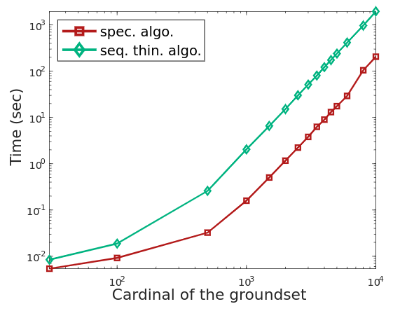 Figure 2
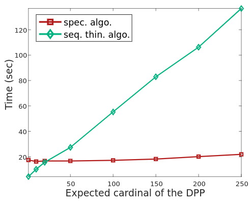 Figure 3
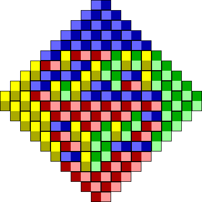 Figure 4
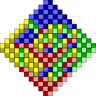 Figure 5
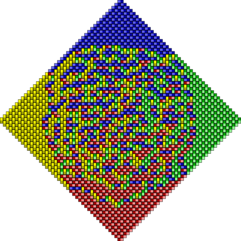 Figure 6
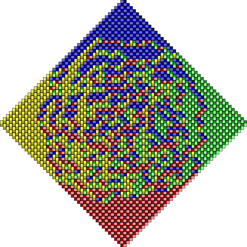 Figure 7
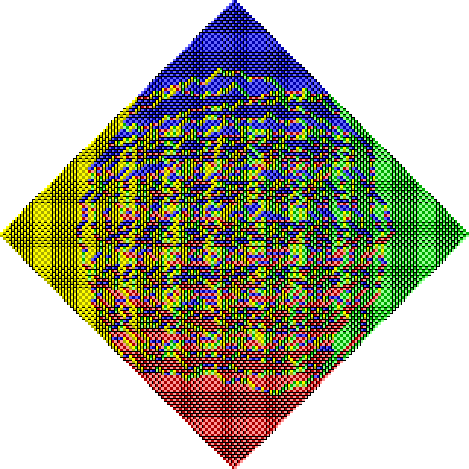 Figure 8
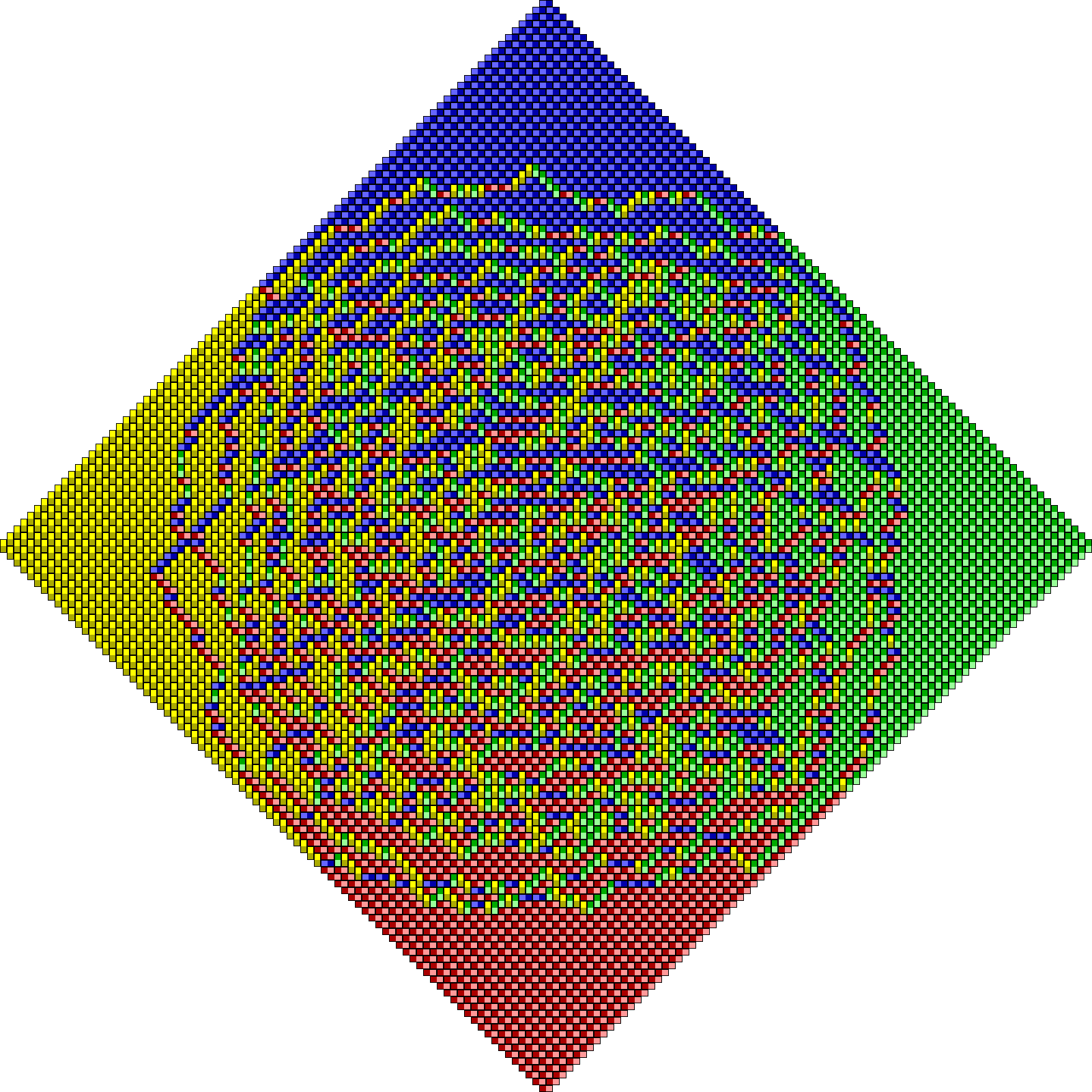 Figure 9
 Figure 10
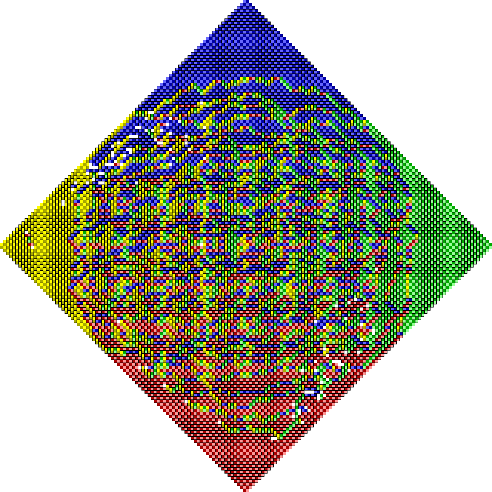 Figure 11
 Figure 12
 Figure 13
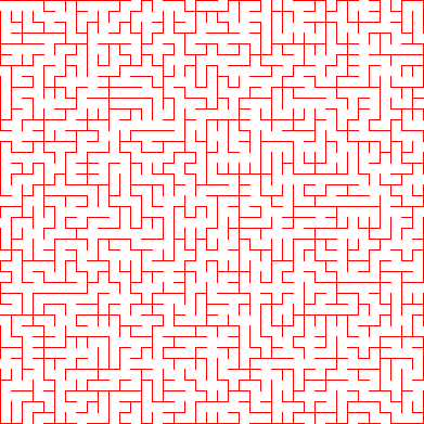 Figure 14
 Figure 15
 Figure 16
 Figure 17
 Figure 18
 Figure 19
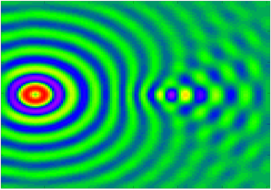 Figure 20
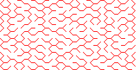 Figure 21
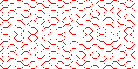 Figure 22
 Figure 23
 Figure 24
 Figure 25
 Figure 26
 Figure 27
 Figure 28
 Figure 29
 Figure 30
Peer Reviews
No public reviews on file for this paper yet. If you reviewed it on a platform where reviews are public (OpenReview, ICLR, NeurIPS, ICML), you can paste yours below so the community can read it here.
Code & Models
Videos
No videos yet. Explain this paper in a talk, walkthrough, or lecture? Add one.
High-performance sampling of generic Determinantal
Point Processes
Jack Poulson111 [email protected], Hodge Star Scientific Computing
Abstract
Determinantal Point Processes (DPPs) were introduced by Macchi [1] as a model for repulsive (fermionic) particle distributions. But their recent popularization is largely due to their usefulness for encouraging diversity in the final stage of a recommender system [2].
The standard sampling scheme for finite DPPs is a spectral decomposition followed by an equivalent of a randomly diagonally-pivoted Cholesky factorization of an orthogonal projection, which is only applicable to Hermitian kernels and has an expensive setup cost. Researchers [3, 4] have begun to connect DPP sampling to factorizations as a means of avoiding the initial spectral decomposition, but existing approaches have only outperformed the spectral decomposition approach in special circumstances, where the number of kept modes is a small percentage of the ground set size.
This article proves that trivial modifications of and factorizations yield efficient direct sampling schemes for non-Hermitian and Hermitian DPP kernels, respectively. Further, it is experimentally shown that even dynamically-scheduled, shared-memory parallelizations of high-performance dense and sparse-direct factorizations can be trivially modified to yield DPP sampling schemes with essentially identical performance.
The software developed as part of this research, Catamari [hodgestar.com/catamari] is released under the Mozilla Public License v2.0. It contains header-only, C++14 plus OpenMP 4.0 implementations of dense and sparse-direct, Hermitian and non-Hermitian DPP samplers.
1 Introduction
Determinantal Point Processes (DPPs) were first studied as a distinct class by Macchi in the mid 1970’s [1, 5] as a probability distribution for the locations of repulsive (fermionic) particles, in direct contrast with Permanental – or, bosonic – Point Processes. Particular instances of DPPs, representing the eigenvalue distributions of classical random matrix ensembles, appeared in a series of papers in the beginning of the 1960’s [6, 7, 8, 9, 10] (see [11] for a review, and [12] for a computational perspective on sampling classical eigenvalue distributions). Some of the early investigations of (finite) DPPs involved their usage for uniformly sampling spanning trees of graphs [13, 14] (see Figs. 1 and 2), non-intersecting random walks [15], and domino tilings of the Aztec diamond [16, 17, 18, 19] (see Figs. 3 and 4).
Let us recall that the class of immanants provides a generalization of the determinant and permanent of a matrix by using an arbitrary character of the symmetric group to determine the signs of terms in the summation:
[TABLE]
Choosing the trivial character yields the permanent, while choosing provides the determinant. The resulting generalization from Determinantal Point Processes and Permanental Point Processes to Immanantal Point Processes was studied in [20].
Definition 1
A finite Determinantal Point Process is a random variable over the power set of a ground set such that
[TABLE]
where is called the marginal kernel matrix and denotes the restriction of to the row and column indices of .
We can immediately observe that the -th diagonal entry of a marginal kernel is the probability of index being in the sample, , so the diagonal of every marginal kernel must lie in . A characteristic requirement for a complex matrix to be admissible as a marginal kernel is given in the following proposition, due to Brunel [22], which we will provide an alternative proof of after introducing our factorization-based sampling algorithm.
Proposition 1** **(Brunel [22])
A matrix is admissible as a DPP marginal kernel iff
[TABLE]
We can also observe that, because determinants are preserved under similarity transformations, there is a nontrivial equivalence class for marginal kernels – which is to say, there are many marginal kernels defining the same DPP:
Proposition 2
The equivalence class of a DPP kernel contains its orbit under the group of diagonal similarity transformations, i.e.,
[TABLE]
If we restrict to the classes of complex Hermitian or real symmetric kernels, the same statement holds with the entries of restricted to the circle group and the scalar orthogonal group , respectively.
Proof.
Determinants are preserved under similarity transformations, so the probability of inclusion of each subset is unchanged by global diagonal similarity. That a unitary diagonal similarity preserves Hermiticity follows from recognition that it becomes a Hermitian congruence. Likewise, a signature matrix similarity transformation becomes a real symmetric congruence. ∎
In most works, with the notable exception of Kasteleyn matrix approaches to studying domino tilings of the Aztec diamond [16, 17, 18, 19], the marginal kernel is assumed Hermitian. And Macchi [1] showed (Cf. [23, 24]) that a Hermitian matrix is admissibile as a marginal kernel if and only if its eigenvalues all lie in . The viewpoint of these eigenvalues as probabilities turns out to be productive, as the most common sampling algorithm for Hermitian DPPs, due to [24] and popularized in the machine learning community by [2], produces an equivalent random orthogonal projection matrix by preserving eigenvectors with probability equal to their eigenvalue:
Theorem 1** **(Theorem 7 of [24])
Given any Hermitian marginal kernel matrix with spectral decomposition , sampling from is equivalent to sampling from a realization of the random DPP with kernel , where consists of the columns of with , independently for each .
Such an orthogonal projection marginal kernel is said to define a Determinantal Projection Process [24], or elementary DPP [2], and it is known that the resulting samples almost surely have cardinality equal to the rank of the projection (e.g., Lemma 17 of [24]). The algebraic specification in Alg. 1 of [2] of the Alg. 18 of [24] involved an approach, where is the rank of the projection kernel. In many important cases, such as uniformly sampling spanning trees or domino tilings, is a large fraction of , and the algorithm has quartic complexity (assuming standard matrix multiplication). In the words of [2]:
Alg. 1 runs in time , where is the number of eigenvectors selected […] the initial eigendecomposition […] is often the computational bottleneck, requiring time. Modern multi-core machines can compute eigendecompositions up to at interactive speeds of a few seconds, or larger problems up to in around ten minutes.
A faster, algorithm for sampling elementary DPPs was given as Alg. 2 of [25]. We will later show that this approach is equivalent to a small modification of a diagonally-pivoted, rank-revealing, left-looking, Cholesky factorization [26], where the pivot index is chosen at each iteration by sampling from the probability distribution implied by the diagonal of the remaining submatrix (which is maintained out-of-place).
As a brief aside, we recall that the distinction between up-looking, left-looking, and right-looking factorizations is based upon their choice of loop invariant. Given the matrix partitioning
[TABLE]
where the diagonal of comprises the list of eliminated pivots: an up-looking algorithm will have only updated (by overwriting it with its factorization), a left-looking algorithm will also have overwritten with the corresponding block column of the lower triangular factor (and with its upper-triangular factor in the nonsymmetric case), and a right-looking algorithm will additionally have overwritten with the Schur complement resulting from the block elimination of .
Researchers have begun proposing algorithms which directly sample from Hermitian marginal kernels by sequentially deciding whether each index should be in the result by sampling the Bernoulli process defined by the probability of the item’s inclusion, conditioned on the combination of all of the explicit inclusion and exclusion decisions made so far. For example, when deciding whether to include index in the sample, we will have already partitioned into a set of included indices, , and excluded indices, . So we must sample index with probability . Directly performing such sampling using formulae for marginal kernels of conditional DPPs is referred to in [3] as sequential sampling (Cf. [4] for greedy, maximum-likelihood inference).
The primary contribution of this manuscript is to show that sequential sampling can be performed via a small modification of an unpivoted factorization process (where is unit lower-triangular and is real diagonal) and to extend them to non-Hermitian marginal kernels using an unpivoted factorization; [27] motivates an algorithm for learning non-Hermitian DPP kernels by their ability to incorporate both attraction and repulsion between items.
It is then demonstrated that high-performance factorizations techniques [28, 29, 30] lead to orders of magnitude accelerations, and that sparse-direct techniques [31, 32, 33] can yield further orders of magnitude speedups.
2 Prototype factorization-based DPP sampling
To describe factorization processes, we will extend our earlier notation that, for an matrix and an index subset , refers to the restriction of to the row and column indices of . Given a second index subset , will denote the restriction of to the submatrix consisting of the rows indices in and the column indices in . And we use the notation to represent the integer range .
Our derivation will make use of a few elementary propositions on the forms of marginal kernels for conditional DPPs. These propositions will allow us to define modifications to the pivots of an LU factorization so that the resulting Schur complements correspond to the marginal kernel of the DPP over the remaining indices, conditioned on the inclusion decisions of the indices corresponding to the eliminated pivots.
Proposition 3
Given disjoint subsets of the ground set of a DPP with marginal kernel , almost surely
[TABLE]
Proof.
If , then almost surely, so we may perform a two-by-two block LU decomposition
[TABLE]
That is a homomorphism yields
[TABLE]
The result then follows from the definition of conditional probabilities for a DPP:
[TABLE]
∎
Proposition 4
Given disjoint and for a ground set of a DPP with marginal kernel , almost surely
[TABLE]
Proof.
[TABLE]
where the last equality makes use of the Matrix Determinant Lemma. The formulae are well-defined almost surely. ∎
Propositions 3 and 4 are enough to derive our direct, non-Hermitian DPP sampling algorithm. But, for the sake of symmetry with Proposition 3, we first generalize to set exclusion:
Proposition 5
Given disjoint subsets , almost surely
[TABLE]
Proof.
The claim follows from recursive formulation of conditional marginal kernels using the previous proposition. The resulting kernel is equivalent to the Schur complement produced from the block LU factorization
[TABLE]
as the subtraction of 1 from each eliminated pivot commutes with the outer product updates. ∎
Theorem 2** **(Factorization-based DPP sampling)
Given a (possibly non-Hermitian) marginal kernel matrix of order , an LU factorization of can be modified as in Algorithm LABEL:lst:unblocked_dpp to almost surely provide a sample from . This algorithm involves roughly floating-point operations, and the likelihood of any returned sample will be given by the product of the absolute value of the diagonal of the result. If the marginal kernel is Hermitian, the work can be roughly halved by exploiting symmetry in the Schur complement updates.
Proof.
We first demonstrate, by induction, that our factorization algorithm samples the DPP generated by the marginal kernel . The loop invariant is that, at the start of the iteration for pivot index , represents the equivalence class of kernels for the DPP over indices conditioned on the inclusion decisions for indices .
Since the diagonal entries of a kernel matrix represent the likelihood of the corresponding index being in the sample, the loop invariant implies that index is kept with the correct conditional probability. Prop. 3 shows that the loop invariant is almost surely maintained when the Bernoulli draw is successful, and Prop. 4 handles the alternative. Thus, the loop invariant holds almost surely, and, upon completion, the proposed algorithm samples each subset with the correct probability by sequentially iterating over each index, making an inclusion decision with the appropriate conditional probability.
The likelihood of a sample produced by the algorithm is thus the product of the likelihoods of the results of the Bernoulli draws: when a draw for a diagonal entry is successful, its probability was , and, when unsuccessful, . In both cases, the multiplicative contribution is the absolute value of the final state of the ’th diagonal entry. ∎
Theorem 2 provides us with another interpretation of the generic DPP kernel admissibility condition of [22]:
Proposition 1 above.
When Algorithm LABEL:lst:unblocked_dpp produces a sample , the resulting upper and strictly-lower triangular portions of the resulting matrix respectively contain the and strictly-lower portion of the unit-diagonal from the LU factorization of . And we have:
[TABLE]
where is the inclusion probability for index , conditioned on the inclusion decisions of indices .
One can inductively show, working backwards from the last pivot, that always being non-negative is equivalent to all potential pivots produced by our sampling algorithm, the set of conditional inclusion probabilities, living in . Otherwise, there would exist an index inclusion decision change which would not change the sign of . ∎
By replacing the Bernoulli samples of algorithm 2 with the maximum-likelihood result for each index inclusion, we arrive at an analogous (approximate) maximum-likelihood inference algorithm.
In both cases, the same specializations that exist for modifying an unpivoted LU factorization into a Cholesky or (unpivoted) or factorization apply to our DPP sampling algorithms. And as we will see in the next two sections, so do high-performance dense and sparse-direct factorization techniques.
As a brief aside, for real matrices, assuming standard matrix multiplication algorithms, the highest-order terms for the operation counts of dense Gaussian Elimination and an MRRR-based [34] Hermitian eigensolver are and [35]. But the coefficient for the Hermitian eigensolver is misleadingly small, as the initial phase of a Hermitian eigensolver traditionally involves a unitary reduction to Hermitian tridiagonal form that, due to only modest potential for data reuse, executes significantly less efficiently than traditional dense factorizations. So-called Successive Band Reduction techniques [36, 37, 38] were therefore introduced as a gambit for trading higher operation counts for decreased data movement and – as a consequence – increased performance.
Theorem 3** **(Factorization-based elementary DPP sampling)
Given a marginal kernel matrix of order which is an orthogonal projection of rank , performing steps of diagonally-pivoted Cholesky factorization, where each pivot index is chosen by sampling from the diagonal as in Algorithm LABEL:lst:unblocked_elementary_dpp, is equivalent to sampling from . This approach has complexity and almost surely completes and returns a sample of cardinality ; the likelihood of the resulting sample is the square of the product of the first diagonal entries of the partially factored matrix.
Proof.
Alg. LABEL:lst:unblocked_elementary_dpp is, up to permutation, algebraically equivalent to the sampling phase of Alg. 2 of [25]: for the sake of simplicity, it assumes the Gramian is preformed rather than forming it on the fly from the factor. That the probability of a cardinality sample is, almost surely, equal to the product of the squares of the first diagonal entries of the result follows from recognizing that the lower triangle of the top-left submatrix will be the Cholesky factor of , and
[TABLE]
∎
The permutations in Alg. LABEL:lst:unblocked_elementary_dpp were introduced to solidify the connection to a traditional diagonally-pivoted Cholesky factorization. There is the additional benefit of simplifying the usage of Basic Linear Algebra Subprograms (BLAS) [39, 40, 41] calls for the matrix/vector products. But the bulk of the work of this approach will be in rank-one updates, which have essentially no data reuse, and are therefore not performant on modern machines, where the peak floating-point performance is substantially faster than what can be read directly from main memory. The Linear Algebra PACKage (LAPACK) [28] was introduced in 1990 as proof that dense factorizations can be recast in terms of matrix/matrix multiplications; we present analogues in the following section, as well as multi-core, tiled extensions similar to [29, 30].
3 High-performance, dense, factorization-based DPP sampling
The main idea of LAPACK [28] is to reorganize the computations within dense linear algebra algorithms so that as much of the work as possible is recast into composing matrices with nontrivial minimal dimensions. Basic operations rich in such matrix compositions – typically referred to as Level 3 BLAS [41] – are the building blocks of LAPACK. In most cases, such block sizes range from roughly 32 to 256, with 64 to 128 being most common.
In the case of triangular factorizations, such as Cholesky, , and LU, a blocked algorithm can be produced from the unblocked algorithm by carefully matricizing each of the original operations. In the case of a right-looking LU factorization without pivoting, one arrives at Alg. LABEL:lst:blocked_lu, where takes the place of the scalar pivot and must be factored – typically, using the unblocked algorithm being generalized – before its components are used to solve against and .
Algorithm 3: Blocked LU factorization without pivoting. The functions triu and unit_tril mirror MATLAB notation and respectively return the upper-triangular and unit-diagonal lower-triangular restrictions of their input matrices. ⬇ 1j := 0
2while j < n:
3
4 ;
5
6
7
8
9
10return sample, A
The correct form of these solves can be derived via the relationship:
[TABLE]
where we used shorthand of the form to represent . An unblocked factorization can be used to compute the triangular factors and of the diagonal block , and then triangular solves of the form and yield the two panels. After forming the Schur complement , the problem has been reduced to an LU factorization with fewer variables – that of . Asymptotically, all of the work is performed in the outer-product updates which form the Schur complements.
The conversion of Alg. LABEL:lst:unblocked_dpp, an unblocked DPP sampler, into Alg. LABEL:lst:blocked_dpp, a blocked DPP sampler, is essentially identical to the formulation of Alg. LABEL:lst:blocked_lu from an unblocked LU factorization. We emphasize that, while it is well-known that factorizations without pivoting fail on large classes of nonsingular matrices – for example, any matrix with a zero in the top-left position – the analogue for DPP sampling succeeds almost surely for any marginal kernel.
Algorithm 4: Blocked, factorization-based, non-Hermitian DPP sampling. For a sample , the returned matrix will contain the in-place factorization of , where is the diagonal indicator matrix for the entries not in the sample, . The usual specializations from to factorization applies if the kernel is Hermitian. ⬇ 1sample := []; A := K; j := 0
2Replace line 5 of main loop of Alg. 3 with:
3
4 sample.append(subsample + j)
5return sample, A
Beyond the order-of-magnitude improvement provided by such algorithms, even on a single core of a modern computer, they also simplify the incorporation of parallelism. Lifting algorithms into blocked form allows for each core to be dynamically assigned tasks corresponding to individual updates of a tile [29, 30], a roughly submatrix which, in our experiments, was typically most performant for .
Within the context of Alg. LABEL:lst:blocked_dpp, our tiled algorithm assigns each unblocked_dpp call an individual OpenMP 4.0 [42] task which depends upon the last Schur complement update of its tile. The triangular solves against are split into submatrices mostly of the form , those of the solves against are roughly of the transpose dimensions, while the Schur complement tasks are roughly of size . In each case, tile reads and writes are scheduled using dependencies on previous updates of the same tile.
The performance of such a dynamically-scheduled parallelization of the Hermitian specialization of Alg. LABEL:lst:blocked_dpp is demonstrated for arbitrary dense, Hermitian marginal kernels on a 16-core Intel i9-7960x in Fig. 5. The performance of a similarly parallelized unpivoted factorization is similarly plotted, and one readily observes that their runtimes are essentially identical. The runtime of Alg. LABEL:lst:blocked_dpp for arbitrary, complex, non-Hermitian marginal kernels is similarly shown in Fig. 6. For purpose of comparison, we note that the double-precision High-Performance LINPACK benchmark [43] achieves roughly 1 TFlop/second on this machine.
It is worth emphasizing the compounding performance gains from both the formulation of DPP sampling as a small modification of a level-3 BLAS focused dense matrix factorization and from the 16-way parallelism. When combined, a factor of 2500x speedup is observed relative to the timings on the same machine of DPPy v0.1.0 [44] when sampling a spectrally-preprocessed arbitrary, dense Hermitian matrix. Similar speedups exist relative to the timings of both the “sequentially thinned” and spectrally-preprocessed algorithms of [3]. In the case of DPPy, it would be fair to attribute at least an order of magnitude of the performance difference to its implementation being standard Python code rather than optimized C++.
In the case of DPPs where the expected number of samples, , is much less than the ground set size, , Derezinski et al. [45] have proposed a rejection-sampling approach with a setup cost of and a subsequent sampling cost of . Ignoring polylogarithmic terms, their setup cost is and the subsequent sampling cost is . Large speedups can therefore be expected when . But the examples in Figs. 1–4 of this article all involve being a modest fraction of , e.g., in the case of the Aztec diamond, so the rejection sampler would involve a prohibitive setup and subsequent sampling cost.
Timings for the and hexagonal-tiling Uniform Spanning Tree DPPs can be extracted from Fig. 5 via the formulae and , respectively, where is the order of the grid. And timings for the uniform domino tilings can be recovered from Fig. 6 via the formula . When computing results for the latter, it was noticed that sampling domino tilings from the Kenyon formula DPP in single-precision, the results are essentially always inconsistent once the diamond size exceeds 60, but no inconsistencies have yet been observed with double-precision sampling. See Fig. 7 for an example.
Such a numerical instability in an unpivoted dense matrix factorization would lead any numerical analyst to wonder if dynamic pivoting can mitigate error accumulation. Indeed, our factorization-based approach frees us to perform arbitrary diagonal pivoting, as long as the pivot is decided before its corresponding Bernoulli draw. While it will be the subject of future work, the author conjectures that maximum-entropy pivoting, that is, pivoting towards a diagonal entry with conditional probability as close to as possible, would be the most beneficial, as it maximizes the magnitude of the smallest possible pivot.
Before moving on to sparse-direct DPP sampling, we demonstrate the multiple orders of magnitude speedup that are possible for Determinantal Projection Processes of sufficiently low rank. Unlike our other experiments, Fig. 8 only executes on a single core, as the unblocked, left-looking rank-revealing elementary DPP sampling approach of Alg. LABEL:lst:unblocked_elementary_dpp spends the majority of its time in matrix/vector multiplication. Studying the benefits of parallelizations of elementary DPP samplers is left for future work.
4 Sparse-direct DPP sampling
As was demonstrated in Fig. 5, the performance of a generic Hermitian DPP sampler can be made to match that of a high-performance Hermitian matrix factorization. This correspondence should not be a surprise, as we have shown that matrix factorizations can be trivially modified to yield Hermitian and non-Hermitian DPP samplers alike. The same insight applies to the conversion of sparse-direct, unpivoted factorization into sparse-direct Hermitian DPP samplers. Such an implementation, mirroring many of the techniques from CholMod [33], was implemented within Catamari.
The high-level approach is to use a dynamically scheduled – via OpenMP 4.0 task scheduling – multifrontal method [46, 32] when the computational intensity of the factorization is deemed high enough after determining the number of nonzeros and of the triangular factor and the number of operations required to compute it. If the arithmetic count and intensity is not sufficiently high, an up-looking, scalar algorithm [33] is used instead.
The multifrontal method performs the bulk of its work processing an (elimination) tree of dense frontal matrices in a post-ordering. Each such frontal matrix for a supernode initially takes the form
[TABLE]
where is the diagonal block of the input matrix corresponding to supernode , is the submatrix of below the supernodal diagonal block that contains at least one nonzero in each row, and the denotes the upper-right quadrant not needing to be accessed due to Hermiticity. Processing such a front involves adding any child Schur complements onto the front, factoring , solving against to replace with , and replacing the bottom-right quadrant with the Schur complement .
This multifrontal process is then parallelized using a tile-based, dynamically scheduled DPP sampler or dense factorization on the diagonal blocks, combined with nested OpenMP tasks launched for each (relaxed) supernode’s [32] subtree [47].
While the author is not aware of any well-studied sparse marginal kernel matrices, [48] proposed a scheme for learning data-sparse marginal kernels defined via Kronecker products and evaluated their technique on the Amazon baby registry dataset of [49]. While DPP learning schemes are beyond the scope of this manuscript, the dramatic factorization speedups that can be supplied by sparse-direct solvers suggests the possibility of learning an entrywise sparse marginal kernel matrix, perhaps via incorporating entrywise soft-thresholding into an iterative learning scheme [49].
We therefore implemented tandem sparse-direct factorization and sparse-direct Hermitian DPP samplers to connect performance results of synthetic sparse DPPs and discretized Partial Differential Equation solvers. Such a statically-pivoted sparse-direct factorization is also the critical computational kernel of primal-dual Interior Point Methods [50, 51], where the first-order optimality conditions are symmetric quasi-semidefinite [52, 53].
Performance results for the dynamically scheduled sparse-direct solver on a 3D Helmholtz equation discretized with trilinear, hexahedral elements Fig. 9 are shown in Fig. 10; results for a 2D DPP analogue, where the marginal kernel takes the form of a scaled 2D Laplacian, are shown in Fig. 11.
In the case of the 2D Laplacian sparse-direct DPP sampling over a grid, the timings were roughly 0.01 seconds on the 16-core i9-7960x. Extrapolating from Fig. 5 to a dense matrix size of , it is clear that several more orders of magnitude of efficiency are gained with the sparse-direct formulation.
We close this section by noting that static pivoting should apply equally well to non-Hermitian sparse-direct DPP sampling, as the nature of small pivots being, by definition, rare, suggests a certain degree of stability. As in the case of dense DPP sampling, probabilistic error analysis is warranted.
5 Conclusions
A unified, generic framework for sequentially sampling both Hermitian and non-Hermitian Determinantal Point Processes directly from their marginal kernel matrices was presented. The prototype algorithm consisted of a small modification of an unpivoted LU factorization – in the Hermitian case, it reduces to a modification of an unpivoted factorization – and high-performance, tiled algorithms were presented in the dense case, and an analogue of CholMod [33] was presented for the sparse case. Further, it was shown that both greedy, maximum-likelihood sampling and elementary DPP sampling can be understood and efficiently implemented using small modifications of traditional matrix factorization techniques.
In addition to generalizing sampling algorithms from Hermitian to non-Hermitian marginal kernels, the proposed approaches were implemented within the open source, permissively licensed, Catamari package and shown to lead to orders of magnitude speedups, even in the dense regime. The Hermitian sparse-direct DPP sampler leads to further asymptotic speedups. Future work includes theoretical and empirical exploration of the stability of dynamic pivoting techniques, both for dense and sparse-direct factorization-based DPP sampling, including the incorporation of maximum-entropy pivoting for large instances of Kenyon-formula Aztec domino tilings.
Further exploration of the performance tradeoffs between left-looking and right-looking elementary DPP sampling, and at which rank it becomes beneficial to use our generic sampling approach, is warranted – especially on multi-core and GPU-accelerated architectures. And, lastly, the incorporation of a tiled extension of [54] for converting a Hermitian L-ensemble kernel into a marginal kernel via [25] is a natural extension of our proposed techniques and could be expected to require the equivalent of 3 samples worth of time due to the computational complexity.
But perhaps the most pressing future direction is to investigate the potential of learning sparse marginal kernels on a benchmark problem, such as the Amazon baby registry of [49]. Ideally such a scheme would expose a roughly block-diagonal covariance matrix which captures item clusters and allows for sufficiently sparse triangular factors.
Reproducibility
The experiments in this paper were performed using version 0.2.5 of Catamari, with Intel’s Math Kernel Library BLAS on an Ubuntu 18.04 workstation with 64 GB of RAM and an Intel i9-7960x processor. Catamari can be downloaded from https://gitlab.com/hodge_star/catamari. Figs. 1 and 2 were generated using the TIFF output from example driver
example/uniform_spanning_tree.cc, while Figs. 3, 4 and 7 similarly used
example/aztec_diamond.cc.
Figs. 5 and 6 were generated using data from example/dense_dpp.cc and example/dense_factorization.cc; we emphasize that explicitly setting both OMP_NUM_THREADS and MKL_NUM_THREADS to 16 on our 16-core machine led to significant performance improvements (as opposed to the default exploitation of hyperthreading). And Fig. 8 was produced with
example/dense_elementary_dpp.cc – with OMP_NUM_THREADS and
MKL_NUM_THREADS explicitly set to one. The algorithmic block_size was also set to a value at least as large as the rank so that a left-looking approach was used throughout.
Figs. 9 and 10 were generated from example/helmholtz_3d_pml.cc, with the 2D-slice of the former taken slightly away from the center plane. Fig. 11 was output from the TIFF support of
example/dpp_shifted_2d_negative_laplacian.cc.
Acknowledgements
The author would like to sincerely thank Guillaume Gautier and Rémi Bardenet for detailed comments on an early draft of this manuscript, as well as their concise explanation of the correctness of the factorization-based sampler at
https://dppy.readthedocs.io/en/latest/finite_dpps/exact_sampling.html#id17. I would also like to thank Jennifer A. Gillenwater for suggesting the conversion from an L-ensemble and Alex Kulesza for answering some of my early DPP questions. Lastly, I am thankful for the insightful comments and suggestions of the two anonymous referees: they significantly improved the quality of the manuscript.
The reference list from the paper itself. Each links out to its DOI / PubMed record.
- 1[1] Odile Macchi. The coincidence approach to stochastic point processes. Advances in Applied Probability , 7(1):83–122, 1975.
- 2[2] Alex Kulesza and Ben Taskar. Determinantal point processes for machine learning. Foundations and Trends in Machine Learning , 5(2–3):123–286, 2012.
- 3[3] Claire Launay, Bruno Galerne, and Agnès Desolneux. Exact Sampling of Determinantal Point Processes without Eigendecomposition. ar Xiv e-prints , page ar Xiv:1802.08429, Feb 2018.
- 4[4] Laming Chen and Guoxin Zhang. Fast greedy map inference for determinantal point process to improve recommendation diversity. In Neur IPS , 2018.
- 5[5] Odile Macchi. The Fermion Process — A Model of Stochastic Point Process with Repulsive Points , pages 391–398. Springer Netherlands, Dordrecht, 1977.
- 6[6] Madan L. Mehta and Michel Gaudin. On the density of eigenvalues of a random matrix. Nuclear Physics , 18:420–427, 1960.
- 7[7] Freeman J. Dyson. Statistical theory of the energy levels of complex systems. i. Journal of Mathematical Physics , 3(1):140–156, 1962.
- 8[8] Freeman J. Dyson. Statistical theory of the energy levels of complex systems. ii. Journal of Mathematical Physics , 3(1):157–165, 1962.
