Property Inference for Deep Neural Networks
Divya Gopinath, Hayes Converse, Corina S. Pasareanu, Ankur Taly

TL;DR
This paper introduces methods to automatically infer formal properties of feed-forward neural networks by analyzing neuron activation patterns, aiding in explanation, robustness, and simplification tasks.
Contribution
It proposes novel techniques to extract input and layer properties from neural networks based on neuron decision patterns, enhancing interpretability and robustness analysis.
Findings
Effective property extraction for MNIST and ACASXU networks
Improved explanation and robustness guarantees
Simplified proofs and network distillation
Abstract
We present techniques for automatically inferring formal properties of feed-forward neural networks. We observe that a significant part (if not all) of the logic of feed forward networks is captured in the activation status ('on' or 'off') of its neurons. We propose to extract patterns based on neuron decisions as preconditions that imply certain desirable output property e.g., the prediction being a certain class. We present techniques to extract input properties, encoding convex predicates on the input space that imply given output properties and layer properties, representing network properties captured in the hidden layers that imply the desired output behavior. We apply our techniques on networks for the MNIST and ACASXU applications. Our experiments highlight the use of the inferred properties in a variety of tasks, such as explaining predictions, providing robustness guarantees,…
Click any figure to enlarge with its caption.
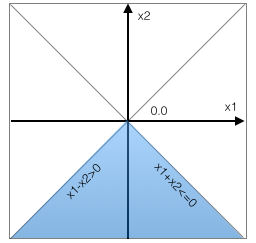 Figure 1
 Figure 2
 Figure 3
 Figure 4
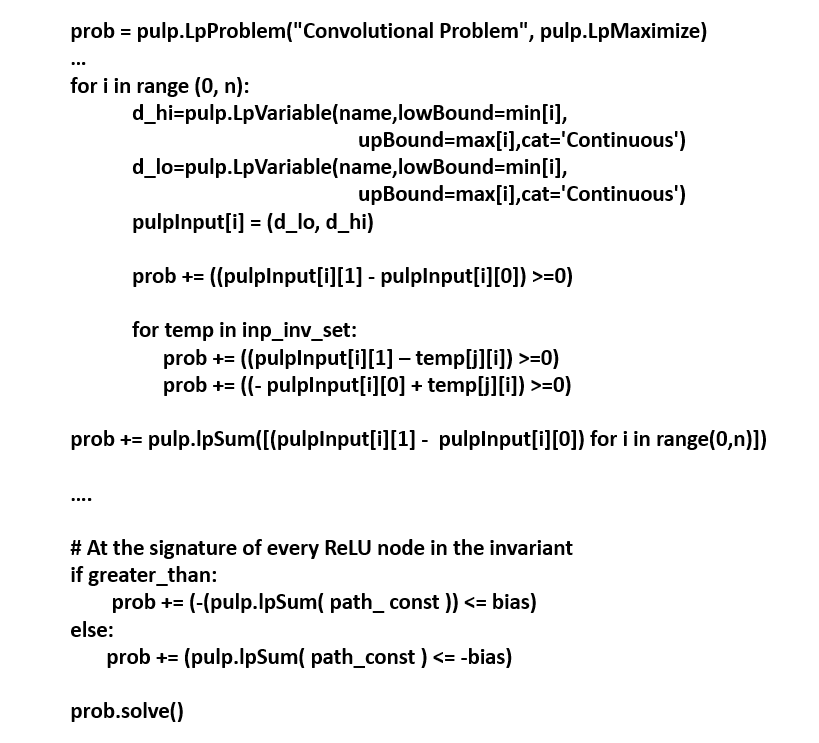 Figure 5
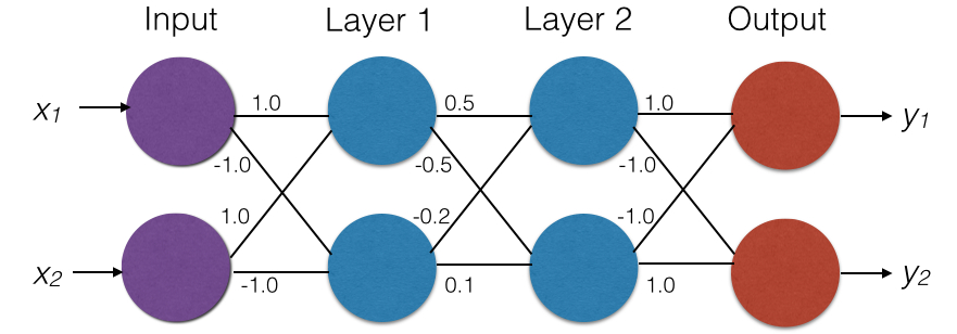 Figure 6
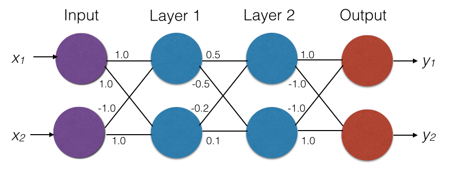 Figure 7
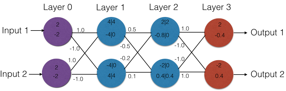 Figure 8
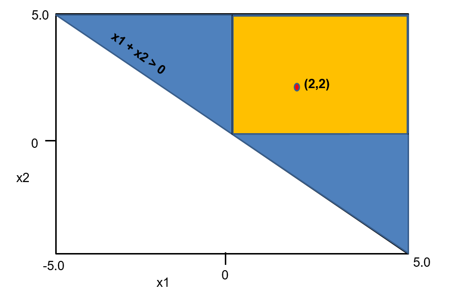 Figure 9
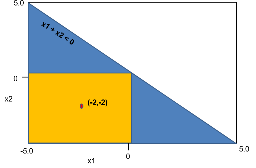 Figure 10
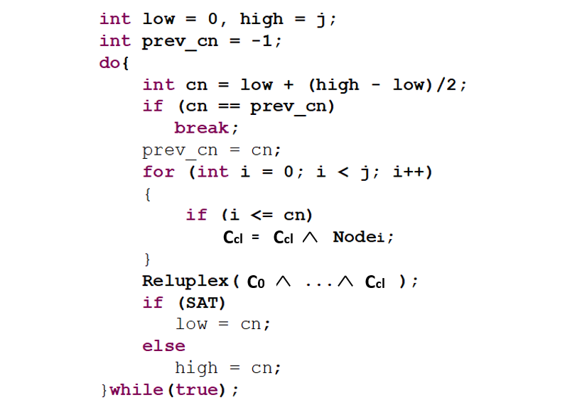 Figure 11
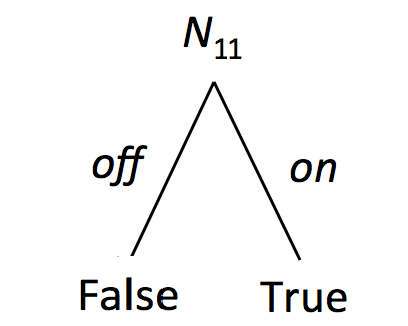 Figure 12
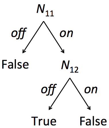 Figure 13
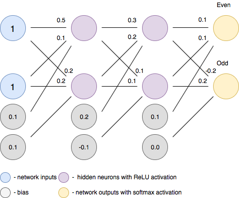 Figure 14
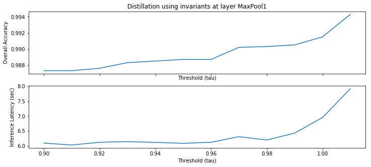 Figure 15
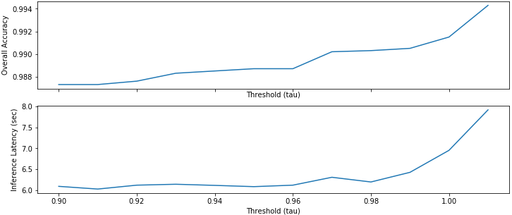 Figure 16
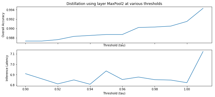 Figure 17
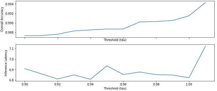 Figure 18
 Figure 19
 Figure 20
 Figure 21
 Figure 22
 Figure 23
 Figure 24
 Figure 25
 Figure 26
 Figure 27
 Figure 28
 Figure 29
 Figure 30
 Figure 31
 Figure 32
 Figure 33
 Figure 34
 Figure 35
 Figure 36
 Figure 37
 Figure 38
 Figure 39
 Figure 40
| Pattern:Label | Layers:Nodes | Support |
|---|---|---|
| : 0 | 1:0-9, 2:0-9 | 1928 |
| : 0 | 1:0-9, 2:0-7 | 2010 |
| : 0 | 1:0-9, 2:0-9 | 217 |
| : 1 | 1:0-9, 2:0-9 | 758 |
| : 1 | 1:0-9, 2:0-5 | 2 |
| : 1 | 1:0-9, 2:0-9, 3:0-9, 4:{5} | 12 |
| : 2 | 1:0-9, 2:{2,3,4,5,8,9} | 1338 |
| : 2 | 1:0-9, 2:0-9, 3:0 | 19 |
| : 2 | 1:0-9, 2:0 | 4 |
| : 3 | 1:0-9, 2:0-9, 3:0-9, 4:{5} | 2 |
| : 3 | 1:0-9, 2:0-9, 3:{3} | 52 |
| : 4 | 1:0-9, 2:0-9, 3:0 | 97 |
| : 4 | 1:0-9, 2:0-9, 3:{4} | 10 |
| : 5 | 1:0-9, 2:0-9, 3:0-9, 4:0-9, 5:0-9, 6:0-1 | 1 |
| : 5 | 1:0-9, 2:0-9, 3:0-9, 4:0-9, 5:{2} | 2 |
| : 6 | 1:0-9, 2:{0,5} | 748 |
| : 6 | 1:0-9, 2:0 | 3904 |
| : 8 | 1:0-9, 2:{0,2,4,5,8} | 358 |
| : 8 | 1:0-9, 2:0-9, 3:0-9, 4:0-9, 5:0-9, 6:0-5 | 3 |
| : 9 | 1:0-9, 2:0-9, 3:0-9, 4:0-2 | 236 |
| : 9 | 1:0-9, 2:0-9, 3:0-9, 4:0-9, 5:0-9, 6:0-9, 7:0-9, 8:0-9, 9:0-9 | 10 |
| : 9 | 1:0-9, 2:0-9, 3:0-9, 4:0-9, 5:0-9, 6:0-9, 7:0-9, 8:0-9, 9:0-9, 10:0-9 | 1 |
| Pattern:Label | Layers:Nodes | Support |
|---|---|---|
| : 6 | 1:0-9 | 3904 |
| : 6 | 7:{1-4, 7, 9} | 5145 |
| : 4 | 6:{0-2, 4-6, 8} | 3078 |
| : 0 | 7:{1-2, 4-5, 7, 9} | 5333 |
| : 0 | 2:0-9, 3:0-7 | 19962 |
| : 3 | 9:{0, 2-4, 6, 8-9} | 3402 |
| : 5 | 10:{0, 2, 4-5, 7-8} | 3075 |
| : 1 | 2:0-9, 3:0 | 18735 |
| Layer | Label | Num of Patterns | Total Supp | MAX supp inv |
|---|---|---|---|---|
| 5 | 0 | 834 | 2237734 | 109147 |
| 5 | 1 | 776 | 3742 | 120 |
| 5 | 2 | 1139 | 7744 | 1324 |
| 5 | 3 | 1745 | 20059 | 2097 |
| 5 | 4 | 1590 | 23580 | 2133 |
| 4 | 0 | 1554 | 208136 | 25489 |
| 4 | 1 | 1185 | 7338 | 732 |
| 4 | 2 | 1272 | 7436 | 745 |
| 4 | 3 | 2322 | 22880 | 1424 |
| 4 | 4 | 2156 | 24565 | 2138 |
| 3 | 0 | 3923 | 249771 | 26134 |
| 3 | 1 | 1906 | 7387 | 210 |
| 3 | 2 | 1866 | 6649 | 134 |
| 3 | 3 | 3420 | 21902 | 945 |
| 3 | 4 | 2932 | 20218 | 552 |
| 2 | 0 | 1924 | 219149 | 51709 |
| 2 | 1 | 734 | 4960 | 497 |
| 2 | 2 | 819 | 4460 | 571 |
| 2 | 3 | 1746 | 14487 | 1262 |
| 2 | 4 | 1640 | 14571 | 1410 |
| 1 | 0 | 2937 | 220395 | 32384 |
| 1 | 1 | 1031 | 4422 | 265 |
| 1 | 2 | 1123 | 3611 | 148 |
| 1 | 3 | 2285 | 11756 | 311 |
| 1 | 4 | 2112 | 11386 | 437 |
Peer Reviews
No public reviews on file for this paper yet. If you reviewed it on a platform where reviews are public (OpenReview, ICLR, NeurIPS, ICML), you can paste yours below so the community can read it here.
Videos
No videos yet. Explain this paper in a talk, walkthrough, or lecture? Add one.
Property Inference for Deep Neural Networks
Divya Gopinath1, Hayes Converse2, Corina S. Păsăreanu1 and Ankur Taly3
1 Carnegie Mellon University and NASA Ames
Email: [email protected],[email protected]
2 University of Texas at Austin
Email: [email protected]
3Google AI
Email: [email protected]
Abstract
We present techniques for automatically inferring formal properties of feed-forward neural networks. We observe that a significant part (if not all) of the logic of feed forward networks is captured in the activation status ( or ) of its neurons. We propose to extract patterns based on neuron decisions as preconditions that imply certain desirable output property e.g., the prediction being a certain class. We present techniques to extract input properties, encoding convex predicates on the input space that imply given output properties and layer properties, representing network properties captured in the hidden layers that imply the desired output behavior. We apply our techniques on networks for the MNIST and ACASXU applications. Our experiments highlight the use of the inferred properties in a variety of tasks, such as explaining predictions, providing robustness guarantees, simplifying proofs, and network distillation.
*Errata: This version updates [14] by correcting the definition of the three properties that were checked for ACASXU in Section V-A. *
I Introduction
Deep Neural Networks (DNNs) have emerged as a powerful mechanism for solving complex computational tasks, achieving impressive results that equal and sometimes even surpass human ability in performing these tasks. However, the increased use of DNNs also brings along several safety and security concerns. These are due to many factors, among them lack of robustness. For instance, it is well known that DNNs, including highly trained and smooth networks, are vulnerable to adversarial perturbations. Small (imperceptible) changes to an input lead to misclassifications. If such a classifier is used in the perception module of an autonomous car, the network’s decision on an adversarial image can have disastrous consequences. DNNs also suffer from a lack of explainability: it is not well understood why a network makes a certain prediction, which impedes on applications of DNNs in safety-critical domains such as autonomous driving, banking, or medicine. Finally, rigorous reasoning is obstructed by a lack of intent when designing neural networks, which only learn from examples, often without a high-level requirements specification. Such specifications are commonly used when designing more traditional safety-critical software systems.
In this paper, we present techniques for automatically inferring formal properties of feed-forward neural networks. These properties are of the form . is a postcondition stating the desired output behaviour, for instance, the network’s prediction being a certain class. is a precondition that we automatically infer and can serve as a formal explanation for why the output property holds. We study input properties which encode predicates in the input space that imply a given output propertyWe further study layer properties which group inputs that have common characteristics observed at an intermediate layer and that together imply the desired output behaviorThe intention is to capture properties based on the features extracted by the network.
There are many choices for defining network properties that are appropriate preconditions for network behavior. In this work, we infer properties corresponding to decision patterns of neurons in the DNN. Such patterns prescribe which neurons are or in various layers. For neurons implementing the activation function, this amounts to whether the neuron output is greater than zero () or equal to zero (). We focus on these simple patterns because they are easy to compute and have simple mathematical representations. Furthermore, they define natural partitions on the input space, grouping together inputs that are processed the same by the network and that yield the same output. Other obvious, more complex properties (e.g. use a positive threshold rather than zero for the activation functions, use linear combinations on neuron values) are left for study in future work.
We define input properties based on patterns that constrain the activation status ( or ) of all neurons up to an intermediate layer. Such patterns form convex predicates in the input space. Convexity is attractive as it makes the inferred properties easy to visualize and interpret. Furthermore, convex predicates can be solved efficiently with existing linear programming solvers. Analogously, we define layer properties based on patterns that constrain the activation status at an intermediate layer. Layer patterns define convex regions over the values at an intermediate layer and can be expressed as unions of convex regions in the input space.
Another motivation for studying decision patterns is that they are analogous to path constrains in program analysis. Different program paths capture different input-output behaviour of the program. Similarly, different neuron decision patterns capture different behaviours of a DNN. It is our proposition that we should be able to extract succinct input-output properties based on decision patterns that together explain the behavior of the network, and can act as formal specifications of networks. We present two techniques to extract network properties. Our first technique is based on iteratively refining decision patterns while leveraging an off-the-shelf decision procedure. We make use of the decision procedure Reluplex [20], designed to prove properties of feed-forward ReLU networks, but other decision procedures can be used as well. Our second technique uses decision tree learning to directly learn layer patterns from data. The learned patterns can be formally checked using a decision procedure. In lieu of a formal check, which is typically expensive, one could empirically validate the learned patterns over a held-out dataset to obtain confidence in their precision.
We consider this work as a first step in the study of formal properties of DNNs. As a proof of concept, we present several different applications. We learn input and layer properties for an MNIST network, and demonstrate their use in providing robustness guarantees, explaining the network’s decisions and debugging misclassifications made by the network. We also study the use of patterns at intermediate layers as interpolants in the proof of given input-output properties for a network modeling a safety-critical system for unmanned aircraft control (ACAS XU) [19]. The learned patterns help decompose the proofs thereby making them computationally efficient. Finally, we discuss a somewhat radical application of the learned patterns in distilling [16] the behavior of DNNs. The key idea is to use the patterns that have high support as distillation rules that directly determine the network’s prediction without evaluating the entire network. This results in a significant speedup without much loss of accuracy.
II Background
A neural network defines a function mapping an input vector of real values to an output vector . For a classification network, the output defines a score (or probability) across classes, and the class with the highest score is typically the predicted class. A feed forward network is organized as a sequence of layers with the first layer being the input. Each intermediate layer consists of computation units called neurons. Each neuron consumes a linear combination of the outputs of neurons in the previous layer, applies a non-linear activation function to it, and propagates the output to the next layer. The output vector is a linear combination of the outputs of neurons in the final layer. For instance, in a Rectified Linear Unit (ReLU) network, each neuron applies the activation function . Thus, the output of each neuron is of the form where are the outputs of the neurons from the previous layer, are the weight parameters, and is the bias parameter of the neuron.111Most classification networks based on ReLUs typically apply a softmax function at the output layer to convert the output to a probability distribution. We express such networks as , where is a pure ReLU network, and then focus our analysis on the network . Any property of the output of is translated to a corresponding property of .
Example.
We use a simple feed forward ReLU network, shown in Figure 1(a), as a running example throughout this paper. The network has four layers: one input layer, two hidden layers and one output layer. It takes as input a vector of size 2. The output vector is also of size 2, indicating classification scores for 2 classes. All neurons in the hidden layers use the ReLU activation function. The final output is a linear combination of the outputs of the neurons in the last hidden layer. Weights are written on the edges. For simplicity, all biases are zero. Consider the input . The output on this input is . To see this, notice that the output of the first hidden layer is . This feeds into the second hidden layer whose output then is . This in turn feeds into the output layer which computes .
A feed forward network is called fully connected if all neurons in a hidden layer feed into all neurons in the next layer; the network in Figure 1(a) is such a network. Convolutional Neural Networks (CNNs) are similar to ReLU networks, but in addition to (fully connected) layers, they may also contain convolutional layers which compute multiple convolutions of the input with different filters and then apply the ReLU activation function. For simplicity, we focus our discussion on ReLU networks, but our work applies to all piece-wise linear networks, including ReLUs and CNNs (and in experiments we describe an analysis for a CNN).
Notations and Definitions. All subsequent notations and definitions are for a feed forward ReLU network , often referred to implicitly. We use uppercase letters to denote vectors and functions, and lowercase letters for scalars. We use to range over neurons, and for the set of all neurons in the network. For any two neurons , the relation holds if and only if the output of neuron feeds into neuron , either directly or via intermediate layers. We define , and extend it to sets of neurons in the natural way.
The output of each neuron can be expressed as a function of the input . We abuse notation and use to denote this function. It is defined recursively via neurons in the preceding layer. That is, if are neurons from the preceding layer that directly feed into , then . For ReLU networks, is always greater than or equal to [math]. We say that the neuron is if and if . This essentially splits the cases when the ReLU fires and does not fire. As we will see in Section III, the / activation status of neurons is our key building block for defining network properties.
III Network Properties
Our goal is to extract succinct input-output characterizations of the network behaviour, that can act as formal specifications for the network. The network itself provides an input-output mapping but of course this is uninteresting. Ideally we should group together inputs that lead to the same output and express that in concise mathematical form. To this end we propose to infer input properties wrt a given output property . An input property is a predicate over the input space, such that, all inputs satisfying it evaluate to an output satisfying the property . In other words, an input property is a precondition for postcondition . Together, the input property and the post condition form a formal contract for the network. An example of an output property for a classification network is that the top predicted class is , i.e., . Such properties are called prediction postconditions.
In this work, we infer input properties that characterize inputs that are processed in the same way by the network, i.e. they follow the same on/off activation pattern up to some layer and define convex regions in the input space. There may be many such convex regions for a particular output property (say a particular prediction). The union of these regions fully captures the behavior of the network wrt the output property. In practice it may be too expensive to compute precisely this union but we show that even computing a subset of these regions can be useful for many applications.
We further study layer properties which encode common properties at an intermediate layer that imply the desired output behavior. Neural networks work by applying layer after layer of transformations over the inputs, to extract important features of the data, and then make decisions based on these features. Thus layer properties can potentially capture common characteristics over the extracted features, allowing us to get insights into the inner workings of the network. Similar to input properties, we seek to infer layer properties by studying the activation patterns of the network. Unlike input properties, layer properties do not map to convex regions in the input space, but rather to unions of convex input regions.
Decision Patterns. We infer network properties based on decision patterns of neurons in the network. A decision pattern specifies an activation status ( or ) for some subset of neurons. All other neurons are don’t care. We formalize decision patterns as partial functions , and write for the set of neurons marked , and be the set of neurons marked in the pattern . Each decision pattern defines a predicate that is satisfied by all inputs whose evaluation achieves the same activation status for all neurons as prescribed by the pattern.
[TABLE]
A decision pattern is a network property wrt a postcondition if:
[TABLE]
We seek minimal patterns which have the property that dropping (which amounts to unconstraining) any neuron from the pattern invalidates it. Minimality helps in getting rid of unnecessary constraints, and ensuring that more inputs can satisfy the property.
The support of a pattern, denoted by , is a measure of the number of inputs that follow the pattern. Formally, it is the total probability mass of inputs satisfying , under a given input distribution. In the absence of an explicit input distribution, support can be measured empirically based on a training or test dataset. For large networks a formal proof for may not be feasible. In such cases, one could aim for a probabilistic guarantee that the conditional expectation (denoted ) of given is above a certain threshold, i.e., .222This is similar to the probabilistic guarantee associated with “Anchors” [29], which we discuss further in Section VI.
III-A Input Properties
To build input properties we infer input properties that are convex predicates in the input space implying a given postcondition. Given that feed forward ReLU networks encode highly non-convex functions, the existence of input properties is itself interesting. To identify input properties, we consider decision patterns wherein for each neuron in the pattern, all neurons that feed into are also included in the pattern. We call such patterns -closed. We show that -closed patterns capture convex predicates in the input space.
Theorem 1
For all -closed patterns , is convex, and has the form:
[TABLE]
Here are some constants derived from the weight and bias parameters of the network.
The proof is provided in the Appendix. It is based on induction over the depth of neurons in the pattern . It shows that the value of any neuron in the pattern can be expressed as a linear combination of the inputs and that each on/off activation adds a linear constraint to the input predicate. 333The theorem can also be proven by representing the network as a conditional affine transformation as shown in [12].
Thus, an input property can be obtained by identifying a -closed pattern such that . For convex postconditions , we show that an input property can be identified using any input whose output satisfies . For this, we consider the activation signature of , which is a decision pattern that constrains the activation status of all neurons to that obtained during the evaluation of .
Definition 1
Given an input , the activation signature of is a decision pattern such that for each neuron , is if , and otherwise.
It is easy to see that is a -closed pattern. Thus, following Theorem 1, can be used to obtain an input property, i.e. a property that implies a desired output behavior. We state this result as a proposition, which will be used in Section IV.
Proposition 1
Given a convex postcondition and an input whose output satisfies (i.e., holds), the following holds. There exist parameters such that:
- (A)
**
- (B)
The predicate is an input property.
Example. We illustrate input properties on the network shown in Figure 1(a) (introduced in Section II). Consider the postcondition that the top prediction is class , i.e., . Let be the neurons in the first hidden layer, and be the neurons in the second hidden layer. Consider the pattern . We argue that this pattern is an input property wrt . Since is it must be the case that the values that feed into (which have the form ) are positive, hence the inputs satisfy . Furthermore, since is it must be the case that the values that feed into (which have the form ) are negative, hence the inputs satisfy . Now notice that all the inputs that satisfy these two constraints also satisfy neuron is always and neuron is always . This is because the value that feeds into is which must be positive (since ). Similarly the value that feeds into is which must be negative. Consequently the output always satisfies (when ), making the pattern a precondition for the property . The pattern is -closed, and therefore by Theorem 2, the predicate is convex. The predicate (see Equation 7) amounts to the convex region (shown in blue in Figure 1(b)) and is minimal.
III-B Layer Properties
While inferred input properties may be easy to interpret, they often have tiny support. For instance, a property defined based on the activation signature of an input may only be satisfied by , and possibly a few other inputs that are syntactically close to . Ideally, we’d like properties to group together inputs that are semantically similar in the eye of the network. To this end, we focus on decision patterns at an intermediate layer that capture high-level features.
A layer property for a postcondition encodes a decision pattern over neurons in a specific layer that satisfies .444For simplicity, we restrict ourselves to computing properties with respect to a single internal layer but the approach extends to multiple layers.
Note that a layer property is convex in the space of values at that layer, but not in the input space. However, it is simple to express a layer property as a disjunction of input preconditions. This is achieved by extending a layer pattern with all possible patterns over neurons that feed into the layer (directly or indirectly). Each such extended pattern is -closed, and therefore convex (by Theorem 2). We formulate this connection between layer and input properties in the following proposition.
Proposition 2
Let be a layer property for an output property . Let be the set of neurons constrained by , and let be all possible decision patterns over neurons in 555There are two such patterns. Then the following statements hold:
- (A)
For each , is an input property.
- (B)
.
Thus, layer properties can be seen as a grouping of several input properties as dictated by an internal layer. We note that identifying the right layer is key here. For instance, if one picks a layer too close to the output then the layer property may span all possible input properties, which is uninteresting. In general, the choice of layer would depend on the application. We discuss it further in Section V.
Example. Let us revisit the example in Figure 1(a) for the postcondition that the top prediction is class , i.e., . A layer pattern for this property is . It is easy to see that for all inputs satisfying this pattern, the output will satisfy , making the pattern a layer property wrt . The pattern is satisfied by the input . The execution of this input involves neuron being and neuron being . Consequently, by proposition 2 (part (A)), the extended pattern is an input property wrt .
III-C Interpreting and Using Inferred Network Properties
Robustness guarantees and adversarial examples. We first remark that provably-correct input and layer properties defined wrt prediction postconditions characterize regions in the input space in which the network is guaranteed to give the same label, i.e. the network is robust. Inputs generated from counter-examples of pattern candidates that fail to prove represent potential adversarial examples, as they are close (in the Euclidean space) to (regions of) inputs that are classified differently. Furthermore, they are semantically similar to benign ones (since they follow the same decision pattern) yet are classified differently. We show such examples in Section V.
Explaining network predictions. Neural networks are infamous for being complex black-boxes [22, 4]. An important problem in interpreting them is to understand why the network makes a certain prediction on an input. Predictions properties (that ensure that the prediction is a certain class) can be used to obtain such explanations. But, such properties are useful explanations only if they are themselves understandable. Inferred input properties are useful in this respect as they trace convex regions in the input space. Such regions are easy to interpret when the input space is low dimensional.
For networks with high-dimensional inputs (e.g., image classification networks) input properties may be hard to interpret or visualize. The conventional approach here is to explain a prediction by assigning an importance score, called attribution, to each input feature [32, 33]. The attributions can be visualized as a heatmap overlayed on the visualization of the input. In light of this, we propose two different methods to obtain similar visualizations from input properties. We note that in contrast to attributions, which help explain predictions for individual inputs, our proposed input properties help explain the predictions for regions of the input space. Furthermore, and in contrast to existing attribution methods, they provide formal guarantees as the computed explanations are themselves network properties that imply the given postcondition.
Under-approximation Boxes.
As stated in Theorem 2, an input property consists of a conjunction of linear inequations, which can be solved efficiently with existing Linear Programming (LP) solvers. We propose computing under-approximation boxes (i.e. bounds on each dimension) as a way to interpret input properties. Specifically, we use LP solving (after a suitable re-writing of the constraints)666We replace each occurrence of variable with or based on the sign of the coefficient in the inequalities. See the Appendix for details on the computation of under-approximation boxes. to find solution intervals for each input dimension such that is maximized. As there are many such boxes, we constrain each box to include as many inputs from the support as possible. These boxes provide simple mathematical representations of the properties, and are easy to visualize and interpret. Note that the under-approximating boxes are themselves network properties that formally imply the input properties and hence the given postcondition.
Minimal Assignments.
We also propose another natural way to interpret both input and layer properties through the lens of a particular input. Analogous to attribution methods, we aim to determine which input dimensions (or features) are most relevant for the satisfaction of the property. Every concrete input defines an assignment to the input variables that satisfies . The problem now is to find a minimal assignment that still leads to the satisfaction of the property, i.e., a minimal subset of the assignments such that . The problem has been studied in the constraint solving literature, and is known to be computationally expensive [3]. We adopt a greedy approach that eliminates constraints iteratively and stops when is no longer implied; the checks are performed with a decision procedure. The resulting constraints are also network properties that formally guarantee the corresponding postcondition.
Layer Patterns as Interpolants. For deep networks deployed in safety-critical contexts, one often wishes to a prove a contract of the form , which says that for all inputs satisfying , the corresponding output () satisfies . For the ACASXU application, there are several desirable properties of this form, wherein, is a set of constraints defining a single or disjoint convex regions in the input space, and is an expected output advisory. Formally, proving such properties for multi-layer feed forward networks is computationally expensive [20]. We show that the inferred network patterns, in particular layer patterns, help decompose proofs of such properties by serving as useful interpolants [24]. Given a layer pattern , we propose the following rule to decompose a proof.
[TABLE]
Thus, to prove , we must first identify a layer pattern that implies output property , and then attempt the proof on the smaller network up to layer . Additionally, once a layer pattern is identified for a property , it can be reused to prove other properties involving . In Section V, we show that this decomposition leads to significant savings in verification time for properties of the ACASXU network.
Distilling rules from networks. Distillation is the process of approximating the behavior of a large, complex deep network with a smaller network [16]. The smaller network is meant to be favorable to deployment under latency and compute constraints while having comparable accuracy. We show that layer patterns with high support provide a novel way to perform such distillation. Suppose is a pattern at an intermediate layer that implies that the prediction is a certain class . For any input , we can execute the network up to layer , and check if the activation statuses of the neurons in layer satisfy the pattern . If they do then we can directly return the prediction class . Otherwise we continue executing the network. Thus for all inputs where the pattern is satisfied, we replace the cost of executing the network from layer onward (possibly involving several matrix multiplications) with simply checking the pattern . The savings could be substantial if layer is sufficiently far from the output, and the layer pattern has high support. Notice that if the patterns are formally verified then this hybrid setup is guaranteed to have no degradation in accuracy. Having said this, we also note that most distillation methods typically tolerate a small degradation in accuracy. Consequently, instead of the expensive formal verification step one could perform an empirical validation of the patterns, and select ones that hold with high probability. This makes the approach practically attractive. As a proof of concept, we evaluate this approach on an eight layer MNIST network in Section V. Interestingly, we note that a network simplified in this manner satisfies the inferred properties by construction, without any proof needed.
IV Computing Network Properties
We now describe two techniques to build input and layer properties from a feed-forward network wrt convex output property .
IV-A Iterative relaxation of decision patterns
This is a technique for extracting input properties. It makes use of an off-the-shelf decision procedure for neural networks. In this work, we use Reluplex [20] but other decision procedures can be used too (see Section VI). 777As discussed, in the absence of a decision procedure, empirical validation of properties can also used. While we would lose the formal guarantee that the computed decision patterns imply the postcondition, they may still be useful in practice.
Recall from Section III that an input property is a -closed pattern that satisfies . Ideally we would like to identify the weakest such pattern, i.e., one that constraints the fewest neurons. Computing such a property would involve enumerating all -closed patterns (), and using a decision procedure to validate whether Equation 2 holds. This is computationally prohibitive.
Instead, we apply a greedy approach to identify a minimal -closed pattern , meaning that there is no -closed sub-pattern of that also satisfies Equation 2. We start with an input whose output satisfies the postcondition , i.e., holds. Let be the activation signature (see Definition 1) of the input . By Proposition 1 (Part (B)), we have that is an input property; recall that is assumed to be convex. But this property may not be minimal. Therefore, we iteratively drop constraints from it till we obtain a minimal property. The algorithm is formally described in the Appendix (see Algorithm 1). It is easy to see that the resulting pattern is , minimal, and it implies the output property ().
Proposition 3
Algorithm 1 (refer Appendix) always returns a minimal input property, and involves at most calls to the decision procedure, where is the number of layers, and is the maximum number of neurons in a layer.
Example. Consider the example network from Figure 1(a), and the input for which the network predicts class . We apply Algorithm 1 to identify an input property for class . The algorithm starts with the activation signature of , which is the pattern . Notice that is already an input property for class . The algorithm begins to unconstrain all neurons in each layer, starting from the last layer, and identifies layer as the critical layer (i.e., unconstraining neurons in layer violates the postcondition). The algorithm then identifies as a minimal pattern that implies the postcondition.
IV-B Mining layer properties using decision tree learning
The greedy algorithm described in the previous section is computationally expensive as it invokes a decision procedure at each step. We now present a relatively inexpensive technique that relies on data, and avoids invoking a decision procedure multiple times. The idea is to observe the activation signatures of a large number of inputs, and learn decision patterns that imply various output properties. In this work, we use decision tree learning (see Appendix for background) to extract compact rules based on the activation statuses ( or ) of neurons in a layer. Decision trees are attractive as they yield decision patterns that are compact (and therefore have high support) based on various information-theoretic measures. The resulting patterns are empirically validated layer properties, which can be formally checked with a single call to a decision procedure.
Our algorithm works as follows. Suppose we have a dataset of inputs . Consider a layer where we would like to learn a layer property wrt postcondition . We evaluate the network on each input , and note: (1) the activation status of all neurons in layer , denoted by , and (2) the boolean indicating whether the output satisfies property . Thus, we have a labeled dataset of feature vectors mapped to labels ; see for example Figure IV-B. We now learn a decision tree from this dataset. The nodes of the tree are neurons from layer , and branches are based on whether the neuron is or . Each path from root to a leaf labeled True forms a decision pattern for predicting the output property; see Figure 2(b). We filter out patterns that are impure, meaning that there exists an input that satisfies but does not hold. The remaining patterns are “likely” layer properties wrt the postcondition. We sort them in decreasing order of their support and invoke the decision procedure () to formally verify them. This last step can be skipped for applications such as distillation (see Section V) where empirically validated patterns may suffice.
We can refine the method for the case where the output property is a prediction postcondition i.e., of the form . In this case, rather than predicting a boolean as to whether the predicted class is , we train a decision tree to directly predict the class label. This lets us harvest layer patterns for prediction postconditions corresponding to all classes. Specifically, the path from the root to a leaf labeled class is a likely layer property for the postcondition that the top predicted class is .
Counter-example guided refinement. In verifying Equation 2 for a decision pattern using a decision procedure, if a counter-example is found, we strengthen the pattern by additionally constraining the activation status of those neurons from layer that have the same activation status for all inputs satisfying the pattern . If verification fails on this stronger pattern then we do a final step of constraining all neurons from layer based on the activation signature of a single input satisfying the pattern. If verification still fails, we discard the pattern. One can also consider a different strategy for refinement, were the counter-examples are added back to the data set and the decision tree learning is re-run, obtaining new layer patterns that will no longer lead to those counter-examples. The drawback is that it may require too many calls to the decision procedure, if many refinement steps are needed.
The reference list from the paper itself. Each links out to its DOI / PubMed record.
- 1[1] N. Carlini and D. Wagner, “Towards evaluating the robustness of neural networks,” in IEEE S&P , 2017.
- 2[2] K. Dhamdhere, M. Sundararajan, and Q. Yan, “How important is a neuron,” in International Conference on Learning Representations , 2019. [Online]. Available: https://openreview.net/forum?id=Syl Koo 0c Km
- 3[3] I. Dillig, T. Dillig, K. L. Mc Millan, and A. Aiken, “Minimum satisfying assignments for smt,” in Proceedings of the 24th International Conference on Computer Aided Verification , ser. CAV’12. Berlin, Heidelberg: Springer-Verlag, 2012, pp. 394–409. [Online]. Available: http://dx.doi.org/10.1007/978-3-642-31424-7_30
- 4[4] B. Doshi-Velez, Finale; Kim, “Towards a rigorous science of interpretable machine learning,” in eprint ar Xiv:1702.08608 , 2017.
- 5[5] S. Dutta, S. Jha, S. Sankaranarayanan, and A. Tiwari, “Output range analysis for deep feedforward neural networks,” in NASA Formal Methods - 10th International Symposium, NFM 2018, Newport News, VA, USA, April 17-19, 2018, Proceedings , 2018.
- 6[6] M. D. Ernst, J. H. Perkins, P. J. Guo, S. Mc Camant, C. Pacheco, M. S. Tschantz, and C. Xiao, “The Daikon system for dynamic detection of likely invariants,” Science of Computer Programming , vol. 69, no. 1–3, pp. 35–45, Dec. 2007.
- 7[7] R. Feinman, R. R. Curtin, S. Shintre, and A. B. Gardner, “Adversarial machine learning at scale,” 2016, technical Report. http://arxiv.org/abs/1611.01236.
- 8[8] M. Fischetti and J. Jo, “Deep neural networks as 0-1 mixed integer linear programs: A feasibility study,” Co RR , vol. abs/1712.06174, 2017.