A Classification of Topological Discrepancies in Additive Manufacturing
Morad Behandish, Amir M. Mirzendehdel, Saigopal Nelaturi

TL;DR
This paper introduces a method to analyze and correct topological discrepancies in additive manufacturing, helping to improve the fidelity of complex 3D printed structures by identifying and addressing defects related to material deposition.
Contribution
It presents a generic topological analysis method for AM discrepancies and demonstrates how to modify structures to preserve topology within printer limitations.
Findings
Effective detection of topological defects in 3D printed structures
Systematic modifications improve structural connectivity
Validated on complex lattice and foam structures
Abstract
Additive manufacturing (AM) enables enormous freedom for design of complex structures. However, the process-dependent limitations that result in discrepancies between as-designed and as-manufactured shapes are not fully understood. The tradeoffs between infinitely many different ways to approximate a design by a manufacturable replica are even harder to characterize. To support design for AM (DfAM), one has to quantify local discrepancies introduced by AM processes, identify the detrimental deviations (if any) to the original design intent, and prescribe modifications to the design and/or process parameters to countervail their effects. Our focus in this work will be on topological analysis. There is ample evidence in many applications that preserving local topology (e.g., connectivity of beams in a lattice) is important even when slight geometric deviations can be tolerated. We first…
Click any figure to enlarge with its caption.
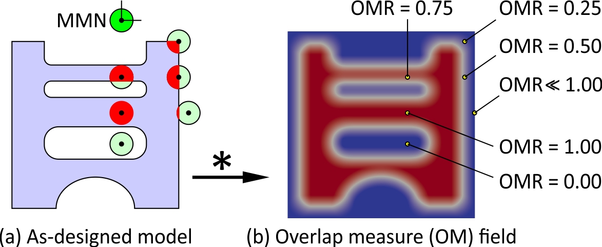 Figure 1
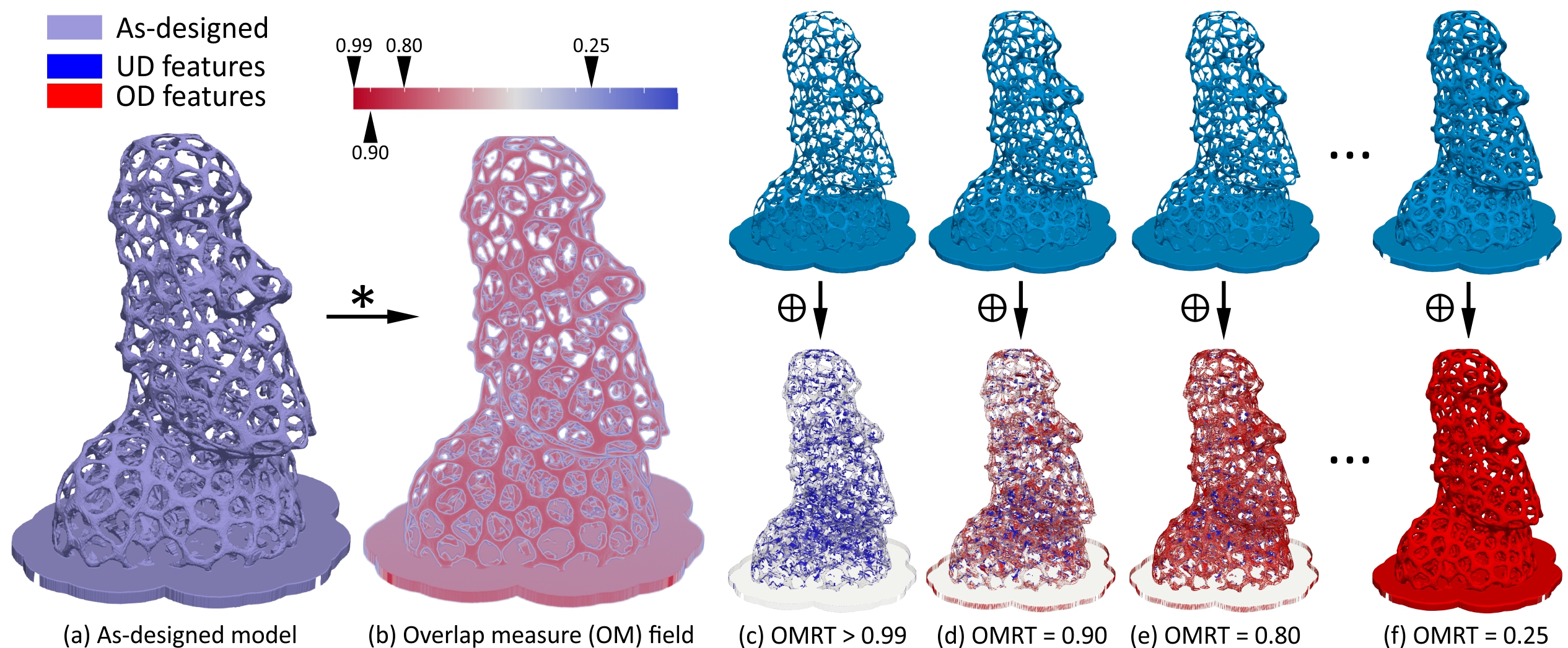 Figure 2
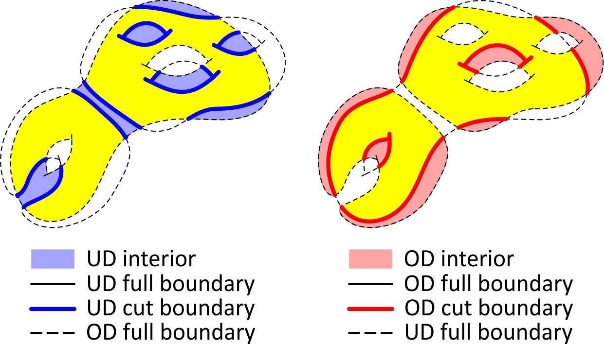 Figure 3
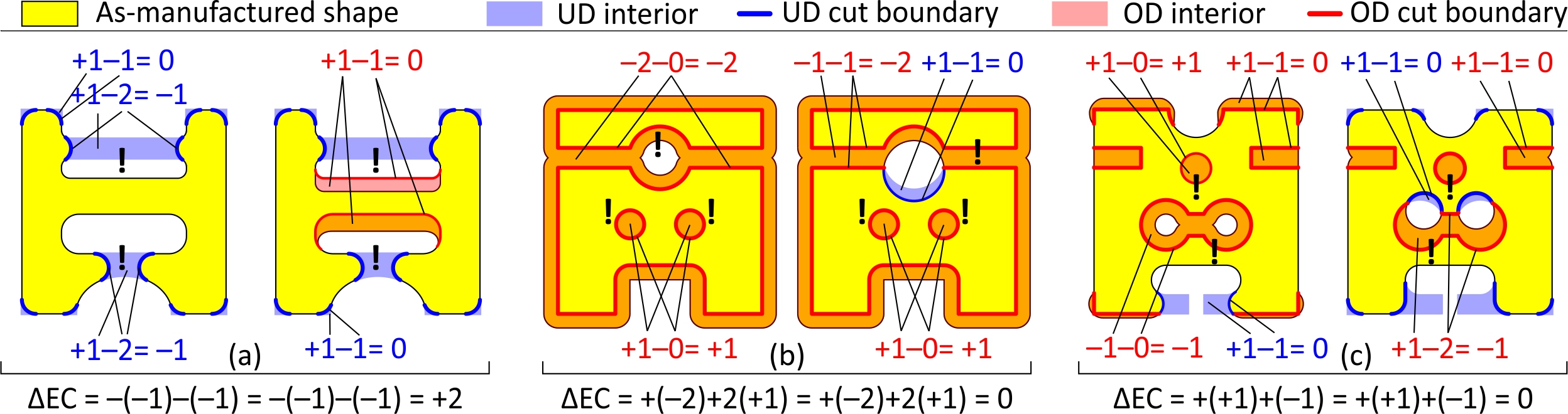 Figure 4
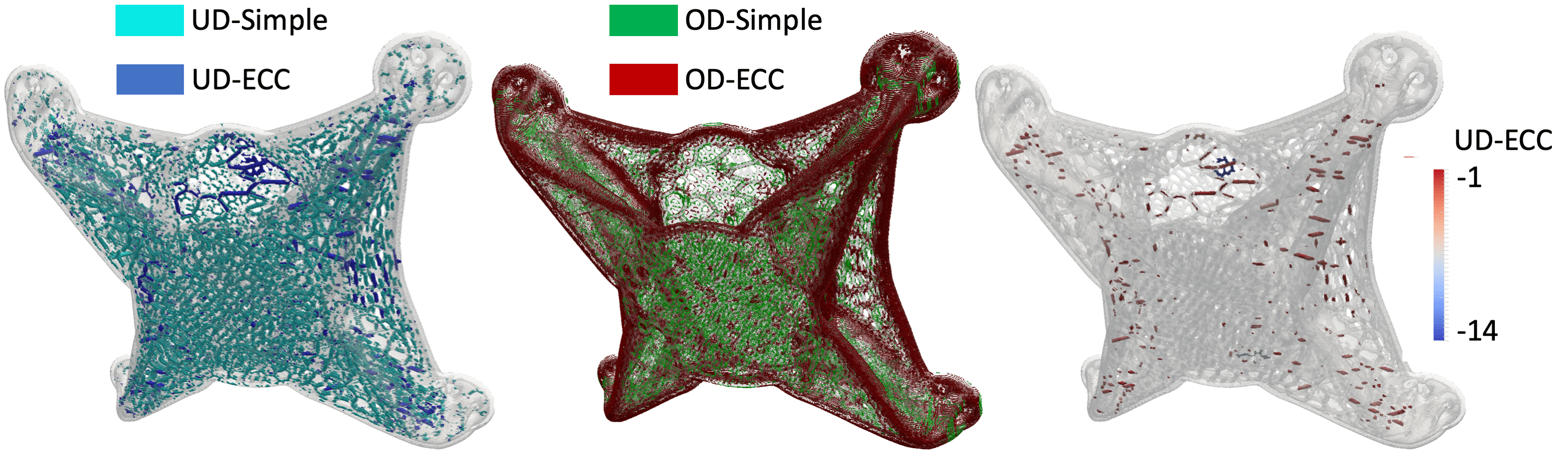 Figure 5
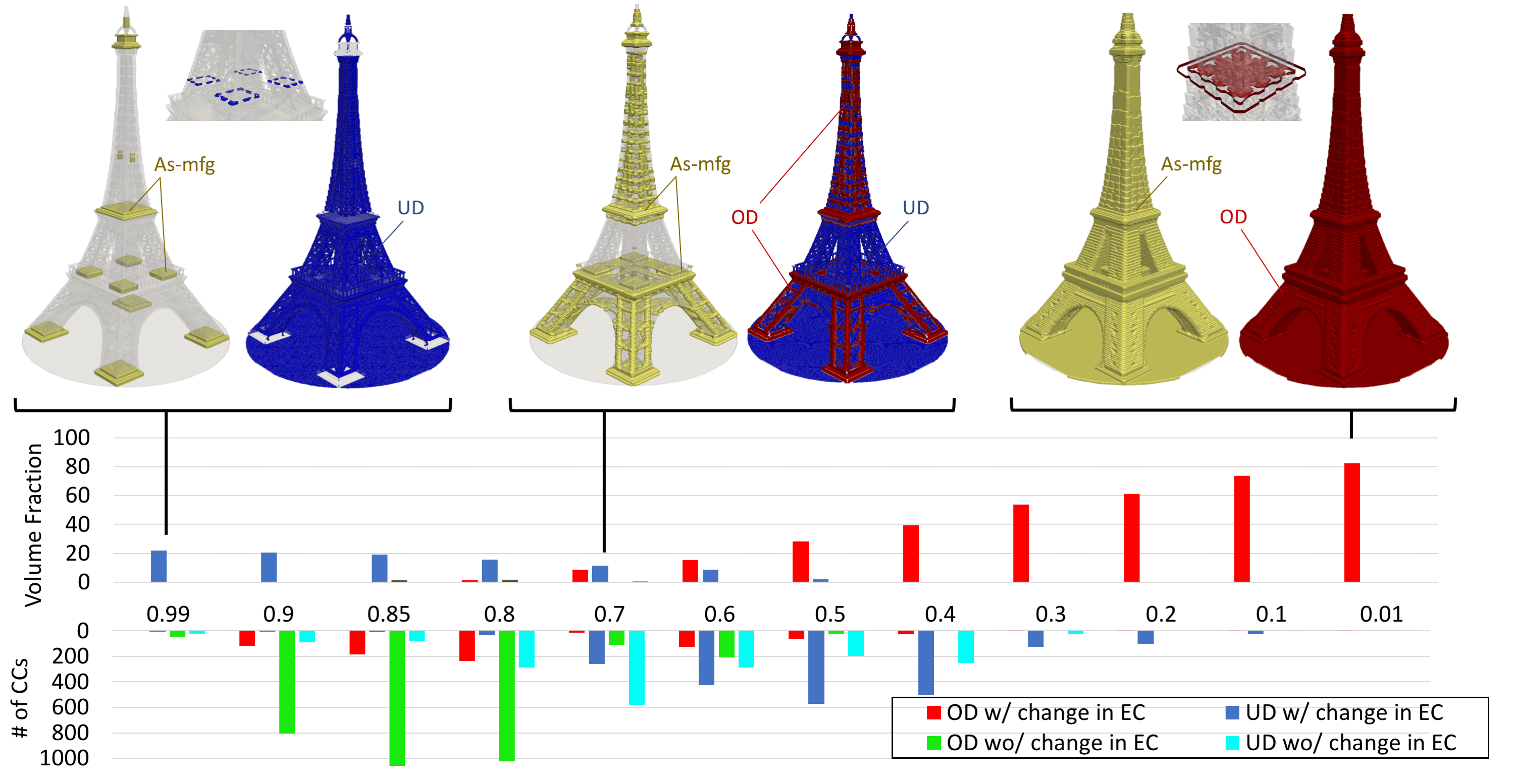 Figure 6
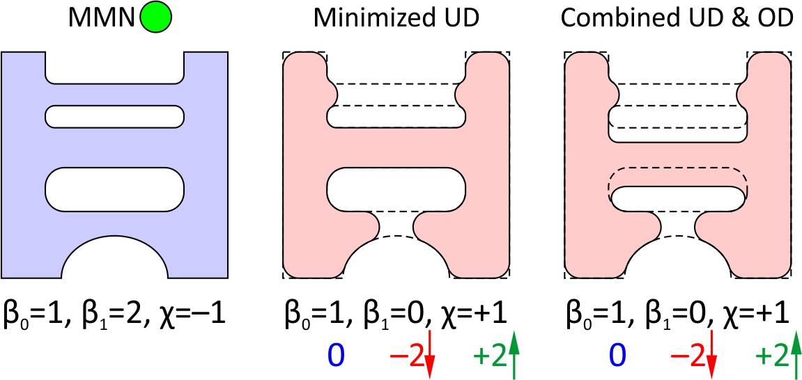 Figure 7
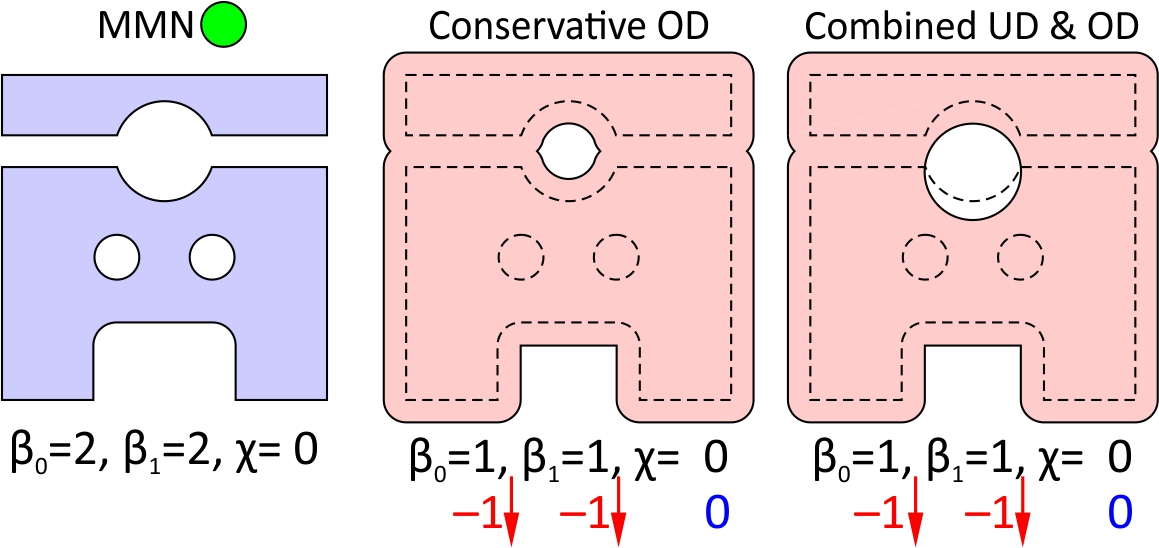 Figure 8
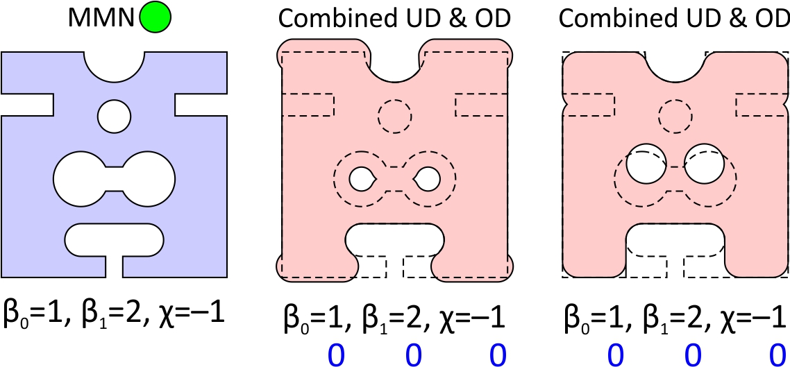 Figure 9
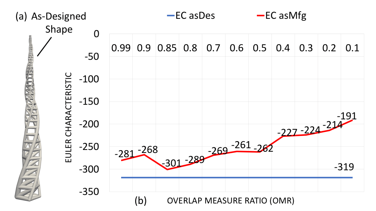 Figure 10
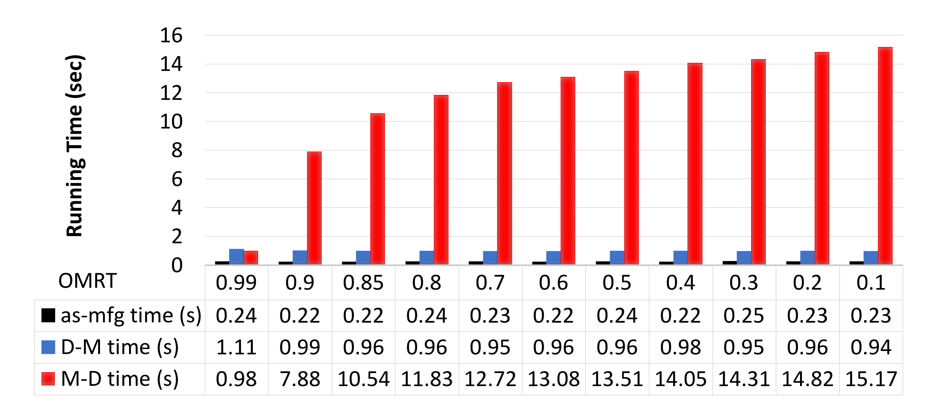 Figure 11
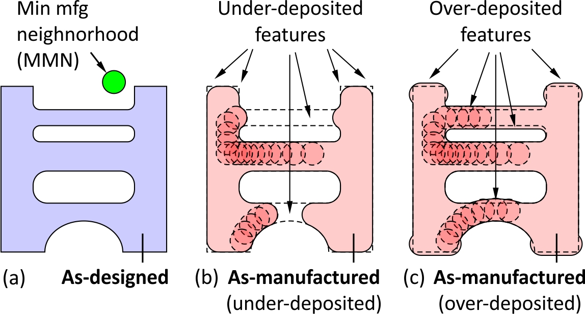 Figure 12
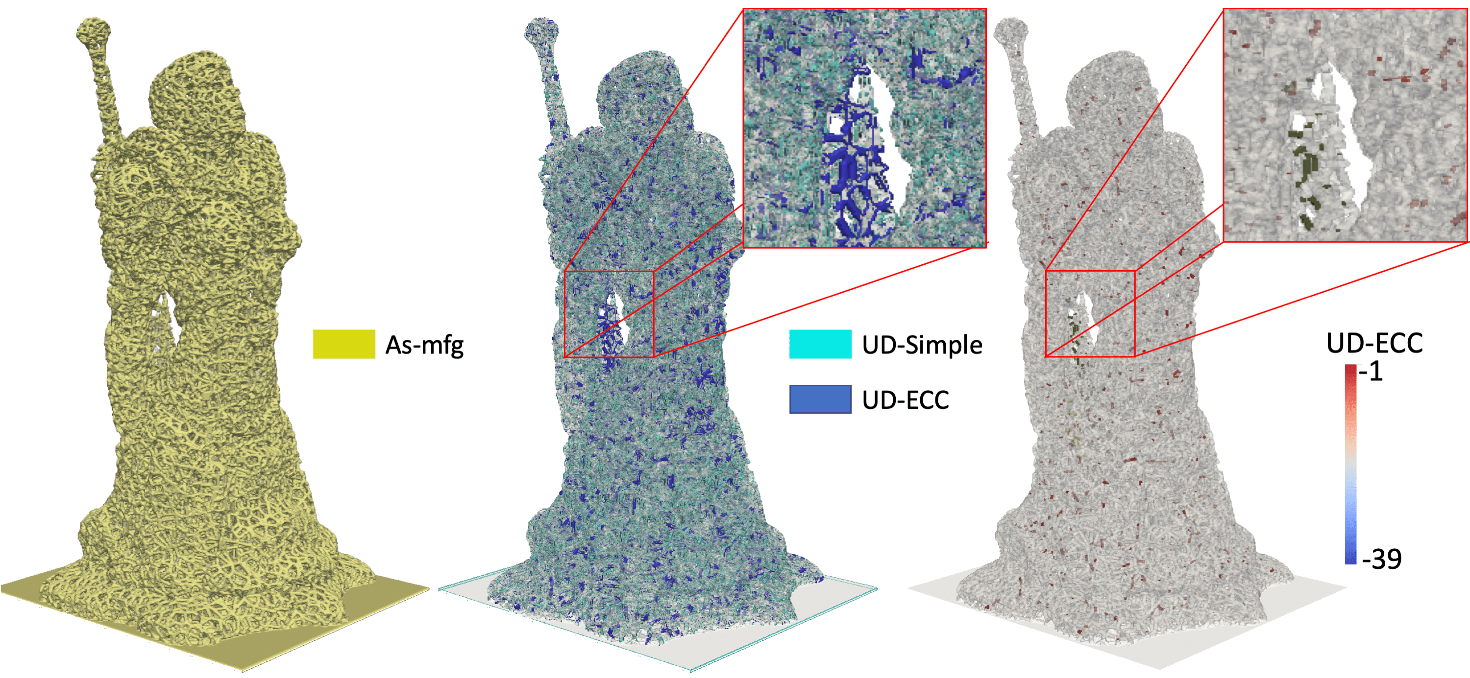 Figure 13
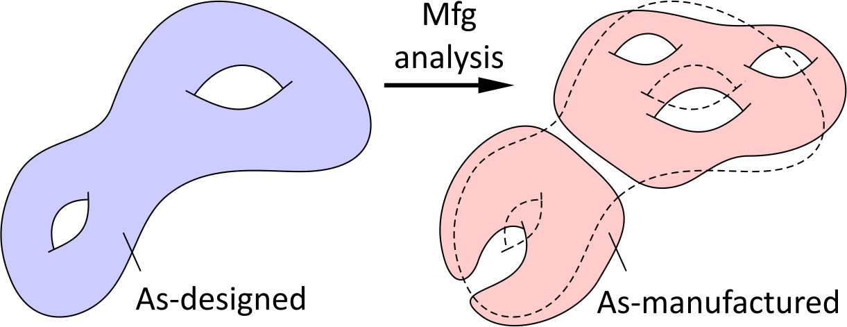 Figure 14
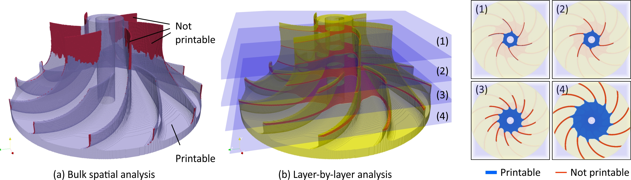 Figure 15
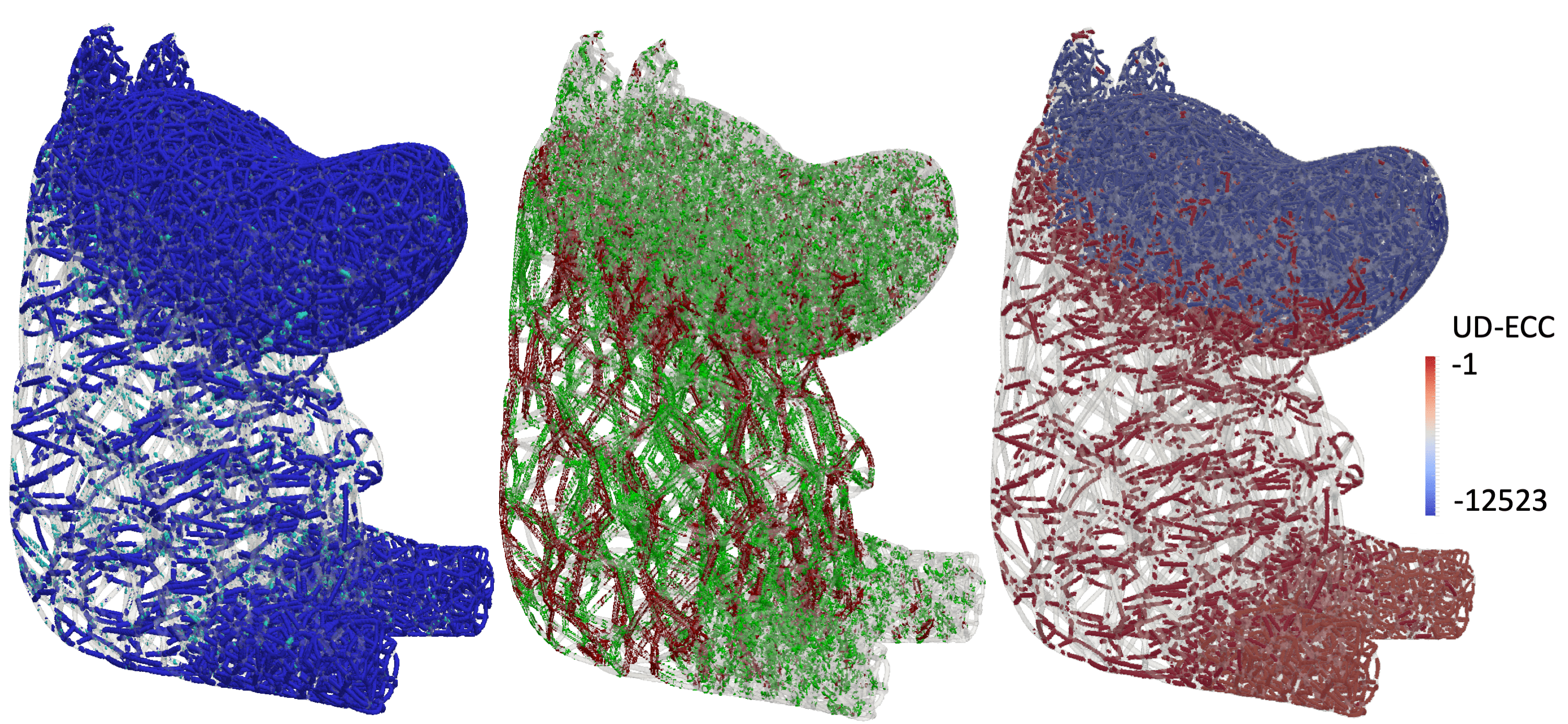 Figure 16
| Example | resolution | UD VF (#CC) | OD VF (#CC) | as-mfg time (s) | UD time (s) | OD time (s) | |
|---|---|---|---|---|---|---|---|
| Knight | 1.33 (6656) | 0 (0) | 0.12 | 3.92 | 0.48 | ||
| Moomin | 10.3 (3659) | 0.63 (2903) | 0.28 | 6.36 | 5.35 | ||
| Copter | 0.36 (1522) | 2.63 (3349) | 0.23 | 2.42 | 9.87 |
Peer Reviews
No public reviews on file for this paper yet. If you reviewed it on a platform where reviews are public (OpenReview, ICLR, NeurIPS, ICML), you can paste yours below so the community can read it here.
Videos
No videos yet. Explain this paper in a talk, walkthrough, or lecture? Add one.
A Classification of Topological Discrepancies in Additive Manufacturing
Morad Behandish, Amir M. Mirzendehdel, and Saigopal Nelaturi
Palo Alto Research Center (PARC), 3333 Coyote Hill Road, Palo Alto, California 94304
Abstract
Additive manufacturing (AM) enables enormous freedom for design of complex structures. However, the process-dependent limitations that result in discrepancies between as-designed and as-manufactured shapes are not fully understood. The tradeoffs between infinitely many different ways to approximate a design by a manufacturable replica are even harder to characterize. To support design for AM (DfAM), one has to quantify local discrepancies introduced by AM processes, identify the detrimental deviations (if any) to the original design intent, and prescribe modifications to the design and/or process parameters to countervail their effects. Our focus in this work will be on topological analysis. There is ample evidence in many applications that preserving local topology (e.g., connectivity of beams in a lattice) is important even when slight geometric deviations can be tolerated. We first present a generic method to characterize local topological discrepancies due to material under- and over-deposition in AM, and show how it captures various types of defects in the as-manufactured structures. We use this information to systematically modify the as-manufactured outcomes within the limitations of available 3D printer resolution(s), which often comes at the expense of introducing more geometric deviations (e.g., thickening a beam to avoid disconnection). We validate the effectiveness of the method on 3D examples with nontrivial topologies such as lattice structures and foams.
keywords:
Additive Manufacturing , 3D Printing , Topological Analysis , Euler Characteristic , Betti Numbers
††journal: Symposium of Solid and Physical Modeling
1 Motivation
Additive manufacturing (AM) has overcome many of the limitations imposed on design by traditional formative and subtractive manufacturing processes. It enables making complex light-weight parts with superior structural [1] or thermal [2] performance, among other functional benefits. The added flexibility and complexity, however, come with a new set of unsolved computational challenges. Often, the as-manufactured structures differ from the as-designed targets in ways that are harder to characterize, quantify, and correct compared to traditional processes such as machining [3]. The deviations depend not only on the geometric and material properties of the part, but also on pre-processing (e.g., slicing and path-planning) and AM process parameters such as build direction, resolution, and temperature. The manufacturing limitations become evident only after the build process is finished [4].
In many cases, the deviations of the as-manufactured structure from the as-designed target are not completely preventable. However, the deviations can be controlled, by slight modification of the design or process, to prevent unpredictable failures. Even when an as-designed target is not manufacturable as-is, there are infinitely many manufacturable alternatives that closely approximate its shape, while preserving the design intent and function. For example, if the as-designed shape has smaller features than the 3D printer’s resolution, there may be many plausible ways to thicken its small structural or aesthetic features with no compromise in its form, fit, and function.
In this paper, we focus on preserving shape properties, particularly those pertaining to topological integrity of the design. For many AM structures (e.g., infill lattices [5, 6] and foams [7, 8]), the topological integrity of the structure has substantial functional significance—commonly even more important than geometric precision. Often times, “small” enough deviations (from a metric standpoint) from the as-designed geometry may lead to changes in topology that compromise performance. For example, if the shape of a lattice structure is slightly deformed due to the stair-stepping effect of layered fabrication, it may not matter as much as preserving its connectivity. Common examples of functional failure are broken beams in load-bearing micro-structures, covered tunnels in heat exchanger micro-channels, filled cavities in porous meta-materials, and so on. Topological properties can impact manufacturing post-processing as well, such as powder removal in SLS or DMLS.
We present a novel approach to detect and classify local contributions to topological discrepancies to enable surgical corrections that preserve the global and local topology.
1.1 Related Work
There are few computational tools for predicting and/or alleviating shape defects introduced by AM. Most of the methods that study the quality of AM processes use geometric measures such as volumetric error [9, 10, 11], dimensional accuracy [12, 13, 14], or surface finish [15] as the main criteria. In other words, feasibility of an AM process for a given design is mainly assessed either through visual and qualitative evaluation [16] or quantitative and statistical analysis on feature sizes and tolerances [17, 18]. For instance [19, 20] demonstrated methods to identify, visualize, and correct thin features in 3D printed parts. However, they offer limited insight on topological consequences of deviations from the original design.
Despite its significance, topology-aware DfAM has received less attention than deserved. For example, a recent study [21] proposed using methods from topological data analysis such as mapper graphs and persistent homology [22] to assess the quality of point cloud data for 3D printing along a given build direction. The method is focused on data quality and representation rather than process effects. Another study [23, 24] proposed a method to restrict enclosed voids in topology optimization. The objective function is penalized by simulated results of artificial heat transfer with large conductivity assigned to the voids. The heuristics are effective in alleviating cavity formations but provide no guarantees. In [19], the authors used medial axes to separate and thicken thin features. Medial axes are hard to compute due to their instability in the presence of noise [25]. In [18], the authors used a different criterion for global thin feature detection based on topological effects of ball inclusion/exclusion. Most existing methods use heuristics for thickening of thin features, rarely consider other classes of features (e.g., tunnels/cavities), and do not quantify the local topological errors in a way that can be used in trade-off with other criteria.
Our goal is to distinguish features (of arbitrary shape) that adversely affect the topology from those that do not. For instance, a missing bridge between two connected components in the as-manufactured shape is qualitatively different from a sharp corner being rounded off without affecting connectivity (Fig. 1). The former changes the local topology, even if the global topology (e.g., total number of connected components) is intact due to possible existence of other connections. Hence, global topological analysis based on Reeb graphs, mapper graphs, persistent homology, and other tools of the trade can miss them.
1.2 Contributions & Outline
This paper presents a novel computational framework to quantify and correct topological discrepancies for AM parts; specifically the contributions of the paper are:
presenting parameterized families of manufacturable alternatives that closely approximate a given design of arbitrary shape for a given AM capability; 2. 2.
quantifying as-manufactured deviations from the as-designed model in terms of under- and over-deposition (UD/OD) regions for every such alternative; 3. 3.
characterizing the local contributions of the deviant UD/OD components to the global topological discrepancies in terms of Euler characteristic (EC); and 4. 4.
prescribing a systematic process to locally adjust the AM instrument motions to counteract the topological deviations with minimal geometric alteration.
In Section 2, we extend previous work on measure-theoretic parametrization of as-manufactured models for a given as-designed model and AM capability [19, 20, 26].
In Section 3, we present a novel approach of comparative topological analysis (CTA) for a pair of arbitrary shapes. We decompose the inevitable discrepancies between the as-designed and as-manufactured shapes due to process limitations into UD/OD “features.” We present a novel computational approach to quantify their local contributions to the global topological changes. Unlike global quantifiers such as the EC and Betti numbers (BN) that count the total number of connected components, tunnels, and cavities in 3D, our analysis provides local and precise spatial information about the comparative topology of the as-designed and as-manufactured shapes.
A theoretical contribution with major computational utility is a general formula to locally quantify topological differences between two arbitrary overlapping shapes. Using the additivity of EC, we define the fundamental notion of (topological) simplicity to decompose and classify the set differences between two arbitrary pointsets.
The classification of local discrepancies is used for surgical modification of the design and process to alleviate undesirable topological discrepancies. We propose a simple approach to locally update the deposition policy while retaining the minimum feature size constraints. The approach can be applied recursively to find the “best” manufacturable approximation to the target design—among many alternatives, as exemplified in Fig. 1—that preserves its topological integrity with the least necessary geometric deviation. However, topological integrity is but one of many (potentially competing) criteria for multi-objective design space exploration [27] and has to be satisfied/optimized for the best trade-offs. Design space exploration is beyond the scope of this paper.
2 Geometric Modeling for AM
In this section, we present a general approach for modeling manufacturable alternatives that closely approximate a given as-designed target of arbitrary shape, while complying with geometric limitations of AM (Section 2.1). Our model offers immense flexibility by generating families of as-manufactured variants over a range of custom AM parameters such as resolution and deposition allowance, rather than a single model (Section 2.2). We conclude this section by a discussion of future directions for extending this model to spatially varying allowance fields to provide additional freedom for local adjustments (Section 2.3).
2.1 From As-Designed to As-Manufactured
Practical limitations on the AM resolution and wall thickness are the source of inevitable geometric and topological discrepancies between the as-designed target and as-manufactured outcome. For example, the layer thickness in direct metal laser sintering (DMLS) is typically in the range 0.3–0.5 mm along the deposition layer and 20–30 microns along the build direction at the highest resolution, with a minimum hole diameter of 0.90–1.15 mm within a typical workspace of mm3. Attempting to fabricate designs that have smaller features will result in disconnected beams, filled holes/tunnels, or hard-to-predict combinations. The as-manufactured part may eventually look nothing like the as-designed target.
As a first approximation, manufacturability analysis can be formulated as a purely geometric problem. Earlier work [19, 20] has developed methods to model as-manufactured structures using basic notions from group morphology [28]. Similar approaches have also been used to generate hybrid (interleaved additive and subtractive) manufacturing process plans [26]. We briefly review the relevant elements of these methods used in this paper.
An as-manufactured shape is obtained by sweeping a minimum manufacturable neighborhood (MMN) of arbitrary shape along an arbitrary motion that is allowed by the machine’s degrees of freedom (DOF) [26]. For example, most 3D printers operate by 3D translations of a printer head (no rotational DOF) over the workpiece as they deposit a droplet of material whose shape is represented by the MMN (e.g., an ellipsoid/cylindroid). The MMN’s size (e.g., diameters/height) and orientation are determined by the printer resolution and the build direction. Unless the as-designed shape is perfectly sweepable by the MMN via an allowable motion, the as-manufactured shape will have to differ. The challenge is to find the “best” allowable motion of the deposition head whose sweep of MMN results in a shape as close as possible to the as-designed target. The answer is not unique, as it depends on the notion of closeness; i.e., the criteria based on which the discrepancies are measured. One such criterion comes from local topological considerations that impact function (Section 3).
2.2 Computing a Family of As-Manufactured Models
For ease of illustration, the examples of this paper are restricted to AM instruments with translational DOF only, i.e., the machine does not allow rotations of the deposition head. This assumption covers commercial 3D printers that deposit flat layers on top of each other. After presenting the results for the simpler case of translations, we also discuss the more general case of general rigid motions supported by high-axis CNC machines.
Manufacturability Measures
Throughout this paper, we adopt a measure-theoretic approach to define and compute as-manufactured shapes. At every point in the 3D space inside the printer workspace—which represents a hypothetical translational configuration of the printer head—we quantify manufacturability by computing the overlap measure (OM) between the stationary as-designed target and a hypothetical MMN instance displaced to the query point. For example, the analysis for 3D printing on flat layers with translational DOF can be performed in at least two ways, as illustrated in Fig. 2:
Bulk spatial analysis: A 3D field of overlap measures is obtained between the 3D as-designed model and a 3D model of the MMN, e.g., a blob of material that is representative of a deposition unit. The layer thickness and build orientation may or may not be encoded into the shape of the MMN. The measure is the volume of intersections between 3D shapes. 2. 2.
Layer-by-layer analysis: The as-designed model is sliced along a fixed build direction into layers that are a constant distance apart, e.g., obtained from a 3D printer’s known layer thickness specs. For each 2D as-designed slice, a 2D field of overlap measure is constructed by using a 2D model of the MMN, e.g., nozzle or laser beam cross-section. The measure is the surface area of intersections between 2D shapes.
(1) provides a rapid approximation to the latter and allows a high-level analysis in the absence of slicing parameters. It can be computed in one shot for digitized translational motions by a convolution of indicator (i.e., characteristic) functions of the as-designed shape and MMN in 3D [20]. On a commodity computer, it can be computed for resolutions of – voxels per coordinate axis due to storage limitations. (2) provides a mid-level analysis that takes build direction and slicing into account, but ignores 1D tool path, digitization (e.g., G-code), and other machine-level details. It can be scaled to resolutions as high as pixels per coordinate axis when each slice is stored and analyzed separately as a bitmap image. For general rigid motions, it is replaced by a parametric motion over a 2D curvilinear surface.
The drawback of (2) is that preserving topological properties per slice does not guarantee preserving topological properties in 3D, which is what matters from a functional standpoint. We will use 2D examples for illustration purposes, and demonstrate 3D examples in Section 4.
Computing AM Instrument Motions
We represent both cases uniformly in terms of Lebesgue measures ( or ) of intersection between the as-designed shape/slice, denoted by and MMN (before displacement), denoted by . These pointsets are assumed to be solids (i.e., ‘r-sets’) [29] defined as compact (bounded and closed) regular and semianalytic subsets of the space, which automatically deems them measurable. We define the OM as a real-valued field over the configuration space (space) of the AM instrument. At a given configuration , the MMN is hypothetically displaced to , where stands for a rigid transformation of . The OM is thus given by .
For example, for axis machines with no rotational DOF (i.e., ), the configurations can be represented by dimensional translation vectors . The displaced MMN is thus obtained as . For high-axis machines with rotations, the instrument configurations are elements of a different subgroup of the 6D Lie group of rigid motions [30], hence the OM is a field defined over a non-Euclidean (Riemannian) manifold. For simplicity, we present the mathematical formula for (translations only) first and briefly discuss extensions, whenever possible, to (combined rotations and translations).
The OM field varies from (no overlap) to the total measure of the MMN (full overlap), the latter corresponding to the configurations (if any) at which the displaced MMN is completely contained within the as-designed shape (i.e., ). The OM ratio (OMR) thus defines a normalized continuous field over the space. The idea is illustrated in Fig. 3 for a 2D example.
Let represent a parametrization that continuously connects the two extremes. We define as a superlevel set of the OM field:
[TABLE]
The members of the family of motions are distinguished by the requirement that for every rigid transformation , the intersection measure between the stationary as-designed shape and the displaced MMN is lower-bounded by a fraction of the maximum possible overlap (Fig. 3). Hereafter, we refer to this fraction as the OMR threshold (OMRT).
At every choice of the OMRT, all configurations whose OMR values exceed the fraction are included in the motion. For purely translational motions (i.e., ), the near-extreme superlevel sets corresponding to can be computed by Minkowski difference/sum, respectively,111We are ignoring the technicalities with regard to regularization of superlevel sets. All equalities are equivalence up to regularization (i.e., equality “almost everywhere” in measure-theoretic sense) [31]. of the as-designed shape with the MMN’s reflection with respect to the origin [19]:
[TABLE]
where denotes a reflection. For other values , , as depicted by Fig. 3. In other words, the one-parametric family of as-manufactured alternatives form a totally ordered set (in terms of containment) bounded by the two extremes given in (2) and (3).
Hereafter, we frequently characterize sets with their defining functions. A real-valued defining function implicitly describes a set as its superlevel set (i.e., ‘support’): For example, describes as:
[TABLE]
where for a given is defined by:
[TABLE]
whose substitution into (4) yields the definition in (1). The indicator (i.e., characteristic) function is a special canonical form of a defining function:
[TABLE]
In general, where for and otherwise.
Next, we transform the above measures into operations on indicator functions of the as-designed shape and MMN. Intersection measures can in general be computed as inner products of indicator functions. If the pointsets are shifted by different relative transformations , the inner product for all translations can be expressed as a single convolution [28]. Hence, for translational motions (i.e., ), the OM can be computed as:
[TABLE]
The MMN measure is simply obtained as a norm of the indicator function . Hence, we rewrite (5) in exact analytical form (i.e., in terms of functions):
[TABLE]
The main advantage of this formulation is its computational efficiency. Convolutions can be computed rapidly via fast Fourier transforms (FFT) [32]. For a grid of size per dimension, this takes , which is very close to linear time in the number of pixels/voxels as opposed to of the naïve approach. When rotations are involved, the above formula holds for every fixed rotation in the space [28], hence the computation is repeated for a sampling of rotations.
For general rigid motions, the above notions are subsumed by Minkowski products/quotients and group convolutions [28]. The general formula is slightly different due to compositions with lifting/projection maps between the Euclidean space and the Lie group . The general idea is nevertheless applicable.
Computing As-Manufactured Shapes
For each set of AM instrument configurations , the resulting as-manufactured shape is obtained by sweeping the MMN along . For purely translational motions (i.e., ) the sweep reduces to a Minkowski sum:
[TABLE]
which extends to Minkowski product for general rigid motion. The defining function of Minkowski sum is also computable as a convolution of indicator functions [28]:
[TABLE]
where the indicator function of is obtained from (6). The as-manufactured shape is obtained as the support of the convolution . Once again, the convolution takes using FFTs, which is only a logarithmic factor away from linear time.
In summary, a one-parametric family of AM instrument motions are computed (for ) as:
[TABLE]
Every is distinguished by its uniform OMRT value of throughout the space. The as-manufactured shape of these motions are then computed as:
[TABLE]
2.3 Modeling Local Geometric Modifications
The one-parametric family of as-manufactured alternatives form a totally ordered set (in terms of containment) bounded by the two extremes; namely,
minimized under-deposition (UD-) () in which the resulting as-manufactured shape is the unique maximal (in terms of containment) manufacturable shape contained within the as-designed shape; and 2. 2.
conservative over-deposition (OD+) () in which the resulting as-manufactured shape is a generalized offset of the as-designed shape with the MMN, and contains the MMN with a conservative margin.
For translational motions, the UD- shape is a morphological opening (i.e., dilation of erosion) while the OD+ shape is a double-offset (i.e., dilation of dilation), obtained by applying (9) to (2) and (3), respectively:
[TABLE]
Figures 3 and 4 illustrate the extreme cases as well as several possibilities in between them, in 2D and 3D, respectively. Decreasing the OMR leads to uniform global thickening of that depends on the local geometry of . If the MMN is small, all alternatives have small geometric deviations from . Nevertheless, they can have dramatically different topological properties (Fig. 4) as we discuss in Section 3.
The choice of OMRT depends on trade-offs between functional requirements. If over-deposition is strictly prohibited, is an obvious choice if the goal is to minimize geometric difference. However, there will be topological consequences due to missing UD features that cause local disconnections (Fig. 4 (c)). If there is some allowance for OD, it is possible to bring those features back by decreasing (Fig. 4 (d–f)). However, the resulting uniform growth of the as-manufactured shape can cause topological errors elsewhere in the shape, such as covering a tunnel/cavity. The geometric allowance may not be uniform either, as functional surfaces may not be grown as much as aesthetic ones. It is possible to extend the above model to accommodate adaptive, non-uniform, and local changes to the as-manufactured shape.
To enable more design freedom, a non-uniform OMRT can be defined as a field and parameterized using a set of basis functions:
[TABLE]
where can be any basis that provides flexible local adjustments (e.g., radial basis functions or splines). The coefficients can be adjusted (e.g., using gradient-descent optimization) based on the feedback from geometric, topological, or physical analysis of the as-manufactured model. Without loss of generality, we let so that the extended model subsumes the uniform OMRT model as a special case when . The extended model is obtained by replacing with in the defining functions of Section 2.2.
Since topological analysis is the main focus of this paper, we postpone a more detailed discussion of as-manufactured shape modeling to future work.
3 Comparative Topological Analysis
We present a novel approach to characterize the differences in basic topological properties of an arbitrary as-designed shape and an as-manufactured shape . The method works for comparative topological analysis (CTA) of arbitrary r-sets , representing the as-designed and (one possible) as-manufactured shape. Note that the latter need not be one of the parametric alternatives presented in Section 2. Our TCA can be applied for an arbitrary the transformation (Fig. 5) that preserves solidity and manifoldness [29].
We quantify the AM-induced discrepancies in terms of the Euler characteristic (EC) and the Betti numbers (BN) (). The two are related in space by a simple linear combination [33]:
[TABLE]
In 2D, and are the numbers of connected components and holes, respectively. In 3D, , , and are the numbers of connected components, tunnels, and cavities, respectively. Intuitively, each counts the number of qualitatively different dimensional closed surfaces contained within the dimensional shape, i.e., surfaces that cannot be transformed to one another via continuous deformations without exiting the shape. Both EC and BN are topological properties in the sense that they are invariant under continuous deformations of the shape itself, which does not apply to the AM process in general (viewed as a transformation ).
3.1 Identifying Local Contributions
Examining global topological changes by comparing the values of (resp. ) with (resp. ) provides little insight into what and how the different geometric features contribute to the discrepancies. Our goal is to quantify local topological discrepancies and identify what features are responsible for them with precise spatial information that can be used for systematic design and process correction. Figures 8, 8, and 8 illustrate a few possible scenarios in 2D when the global analysis is insufficient (e.g., overall EC and/or BNs remain unchanged).
UD/OD Deviation “Features”
Let be the region of space that is common between as-designed and as-manufactured shapes. The set differences between these shapes amount to the under- and over-deposition (UD/OD) regions, denoted respectively by :
[TABLE]
we need to carefully distinguishing regularized set operations (denoted via asterisk) from ordinary set operations. Here, stand for regularized set intersection and set difference [34] which ensure the resulting set is regularized (i.e., “dangling” surfaces/edges are removed).222We do not need to worry about the set union operation, because the union of closed-regular sets is always closed-regular [29]. Hence, regularized set union can be replaced with ordinary set union when both participants are closed-regular sets (e.g., r-sets). The as-designed and as-manufactured shapes can be related set-theoretically as follows:
[TABLE]
If the as-manufactured shape is reasonably close to the as-designed shape, the OD/UD pointsets are made of small and scattered pieces, as we illustrate with examples. Let us decompose the OD/UD pointsets into their respective (disjoint) connected components (CC):
[TABLE]
Note that the CCs do not even touch along boundaries, hence their ordinary pairwise intersections are empty.
Local Topology of the Features
EC is an additive property, i.e., for every pair of (potentially intersecting) pointsets with well-defined ECs, we have:
[TABLE]
Note that even if the two shapes are closed-regular, the intersection is not regularized, and can have lower-dimensional regions such as surface patches, curve segments, and points. As long as the sets are semianalytic, these features are well-behaved with computable ECs. Applying (22) to both sides of (18) and (19) yields:
[TABLE]
Subtracting (24) from (23) eliminates the EC of the common region and yields:
[TABLE]
The terms and can be expanded further (using (22)) in terms of the CCs of and in (20) and (21):
[TABLE]
noting that the components are mutually exclusive, i.e., hence for every pair of indices .
The remaining terms in (25) are the ECs of the pointsets and . These pointsets consist of lower-dimensional regions over which the UD/OD regions intersect the common region . They comprise portions of the boundaries and , as illustrated in Fig. 9. For r-sets, which are assumed to be semianalytic in solid modeling [29], these intersection terms can be stratified into a combination of , , and strata, i.e., surface patches, curve segments, or points, respectively.
Lemma 1**.**
(Euler Characteristic of Cut Boundaries)
[TABLE]
Proof.
For every pair of solids and whose regularized set intersection is empty , their ordinary set intersection can only occur over their common portion of boundaries, leading to the following identities:333In measure-theoretic terms, which, in turn, can be expressed as an inner product .
[TABLE]
which may or may not be empty. We refer to this pointset as the cut boundary of B with A (or vice versa) and denote it by .
The above identity is always true if we let and or , noting that as a result of the definition in (17). Hence:
[TABLE]
Noting that the boundary of the union of disjoint CCs is the same as the union of their boundaries, we obtain:
[TABLE]
Using distributivity of intersection over unions, we obtain:
[TABLE]
Note that (30) holds for and or as well, since for all or , respectively. Hence:
[TABLE]
Applying (22) to both sides of the above equations and noting that the cut boundaries and are all mutually disjoint, we obtain:
[TABLE]
which is the same as (28) and (29). ∎
The following key result follows from substituting the ECs from (26), (27), (28), and (29) into (25):
Corollary 1**.**
(Local Contributions to Global EC)
[TABLE]
The above result motives the following definition of a deviation “feature” for AM processes:
Definition 1**.**
(Deviation Features) A UD/OD ‘deviation feature’ as a pair , where is its solid component and is its cut boundary with another solid such that .
We can also define the notion of EC contribution (ECC) for features in order to simplify (41):
[TABLE]
The feature is called ‘simple’ with respect to a set such that (or simple for short) if .
To summarize, we proved that the total change of EC due to AM errors can be obtained from a sum of contributions of ECs of individual UD/OD features:
[TABLE]
where is the total number of features. The sign depends on the UD/OD type of each feature.
- •
UD features are where stands for the i$${}^{\text{th}} CC of and is its cut boundary with . They contribute to the total change of EC.
- •
OD features are where stands for the i$${}^{\text{th}} CC of and is its cut boundary with . They contribute to the total change of EC.
Corollary 2**.**
A feature does not contribute to the topological change (in terms of EC) from to iff it is simple with respect to .
The above results provide a mechanism to order the UD/OD features in terms of their topological significance. Each feature’s ECC ( or ) to the global variation (i.e., the terms on the right-hand side of (41)) is computed in parallel by subtracting the EC of its cut boundary from the EC of its solid part. Simple features do not contribute anything.
Figure 10 illustrates in 2D how the EC contributions are used to distinguish between simple features such as a rounded corner and non-simple features such as broken beams and filled holes. Even for situations in which there is no change in the total EC (i.e., the left-hand side of (41) or (42) vanished), the analysis reveals how different features cancel each other’s additive contributions. Each feature can thus be corrected independently, within the limitations of the AM process, to achieve an as-manufactured shape that is both globally and locally equivalent to the as-designed shape.
3.2 Correcting Design and Process
Once the contributions of different UD/OD features to the overall EC are determined, the deposition policy can be changed locally to modify the AM instrument’s motion and its resulting as-manufactured shape:
- •
Simple UD/OD features do not contribute anything to the global EC (i.e., ), hence need not be corrected as far as the EC is of concern.
- •
If a UD feature contributes , it should be brought back to by including AM instrument configurations whose sweep of MMN deposits in that region, without affecting other regions.
- •
If an OD feature contributes , it should be eliminated from by excluding AM instrument configurations whose sweep of MMN deposits in that region, without affecting other regions.
Common examples in 3D are (recalling (16)):
- •
A bridge whose solid component is simply-connected (i.e., ) but connects locally disconnected regions in through simply-connected surfaces (i.e., ). Hence we have .
- •
A tunnel whose solid component is simply-connected (i.e., ) but has a cut boundary with that is fully-cylindrical (i.e., ). Hence we have .
- •
A cavity whose solid component is simply-connected (i.e., ) but has a cut boundary with that is fully spherical (i.e., ). Hence we have .
If these features were under- or over-deposited—i.e., either existed in but are missing from (UD), or were not part of but appeared in (OD)—they will contribute a nonzero EC to the total EC.
Once the problematic (i.e., non-simple) features are identified and ranked based on their ECCs, we can make local adjustments to the AM instrument’s motion, such that its resulting sweep of MMN in (9) includes/excludes UD/OD features of topological consequence.
- •
For every non-simple UD feature , we locally decrease the OMRT field in (15) by adjusting the weights, so that it includes configurations in the vicinity of the originally under-deposited region.
- •
For every non-simple UD feature , we locally increase the OMRT field in (15) by adjusting the weights, so that it excludes configurations in the vicinity of the originally over-deposited region.
Every update of the OMRT field results in an updated AM instrument motion, hence a new as-manufactured shape. Adding/removing non-simple UD/OD features can have side effects on other UD/OD features. However, if the modifications are small enough, the classification of features may not change dramatically and the model can be corrected after several iterations. In the interest of keeping this paper short and focused, we will discuss iterative design and process correction elsewhere.
4 Results
In this section, we show examples of applying the developed analysis of Sections 2 and 3 to complex 3D structures. The implementation is in C++ (on Linux). All 3D models (except Fig. 12) are obtained from GrabCAD (https://grabcad.com) and Thingiverse (www.thingiverse.com) and are visualized using ParaView (www.paraview.org).
Figure 12 (a) shows a helical lattice in 3D with as-designed EC of . The global ECs for as-manufactured variants obtained from the one-parametric formula in (12) are plotted in Fig. 12 (b) against the global OMR threshold changing from (minimized UD) to (conservative OD). UD results in larger number of disconnected regions, hence an increase in the (negative) EC. However, as the allowance for OD increases by reducing the OMR, we have both UD/OD that alleviate the increase in number of components while decreasing the number of tunnels with competing effects on EC due to (16). We could apply persistent homology [22] to get a better understanding of the critical OMR values for the birth/death of these topological features. However, the global EC/BN plots or persistence graphs/barcodes lack spatial information needed for design correction.
Figure 12 illustrates the CPU times for parallel computation of ECC for UD/OD features. Notice that as the allowance for over-deposition is increased by decreasing the OMRT, the time increases almost linearly with the overlap measure, which is proportional to the volume (and number of voxels) for OD deviations from design.
The Eiffel tower is an interesting structure with features at different size scales. Figure 13 shows the effect of OMRT on the generation of UD/OD features. Figures 14 and 15 illustrate topological analysis on high-resolution geometries with intricate interior lattices. Table 1 summarizes the results for the three shapes, including running times.
5 Conclusion
A design’s manufacturability (via an AM process) is largely determined by the AM machine’s ability to print the shape within ‘acceptable limits’. The notion of geometric dimensioning and tolerancing has been used successfully to define and check these limits for conventionally manufactured parts, but it is challenging to define features of size for AM, and efforts are ongoing. Nonetheless it is clear that combinations of manufacturing plans and 3D printer resolutions will produce deviations between as-designed and as-manufactured shapes, with no systematic procedure to check and control this deviation.
In this paper we have demonstrated an approach to topologically analyze and classify the deviations between as-designed and as-manufactured shapes. The approach uses fundamental properties of the Euler characteristic to quantify the additive contributions of disjoint regions of over/under-deposition. Ambiguities of global topological analysis arising from the canceling effects of these regions on the local topological changes are resolved. Important geometric features that appear/disappear or are otherwise deformed are identified. The precise spatial information is used to provide remedial measures to retain the geometric feature and the local topology.
Our comparative topological analysis (CTA) in Section 3 is independent of any particular method of computing as-manufactured shapes, hence is not limited to the measure-theoretic model presented in Section 2. Different AM processes may require domain-specific simulation methods that take into account additional process constraints such as solidification, build orientation, support structure, chamber temperature, and so on.
There are several possible extensions to this paper. Our approach considers a single as-manufactured outcome at a time. It provides little insight on the persistence of local changes across the spectrum of as-manufactured variants that one can obtain by changing the 3D printer specs or deposition policies—e.g., by changing the shape/size of MMN, threshold on OMR, etc.
As opposed to analyzing a given as-manufactured model for topological consistency, we may alternatively try to construct a process plan that considers topological changes and produces a part that will (by construction) be topologically equivalent to the as-designed shape.
Solving this problem will also help address broader challenges in design for additive manufacturing (DfAM).
Acknowledgement
This research was developed with funding from the Defense Advanced Research Projects Agency (DARPA). The views, opinions and/or findings expressed are those of the authors and should not be interpreted as representing the official views or policies of the Department of Defense or U.S. Government.
The reference list from the paper itself. Each links out to its DOI / PubMed record.
- 1[1] J. Robbins, S. J. Owen, B. W. Clark, T. E. Voth, An efficient and scalable approach for generating topologically optimized cellular structures for additive manufacturing, Additive Manufacturing 12 (2016) 296–304.
- 2[2] J. H. K. Haertel, G. F. Nellis, A fully developed flow thermofluid model for topology optimization of 3D-printed air-cooled heat exchangers, Applied Thermal Engineering 119 (2017) 10–24.
- 3[3] J. Balic, Intelligent CAD/CAM systems for CNC programming—an overview, Advances in Production Engineering & Management 1 (1) (2006) 13–22.
- 4[4] H. Nouri, S. Guessasma, S. Belhabib, Structural imperfections in additive manufacturing perceived from the X-ray micro-tomography perspective, Journal of Materials Processing Technology 234 (2016) 113–124.
- 5[5] J. Wu, X. Wang, C. C. L .and Zhang, R. Westermann, Self-supporting rhombic infill structures for additive manufacturing, Computer-Aided Design 80 (2016) 32–42.
- 6[6] J. Wu, N. Aage, R. Westermann, O. Sigmund, Infill optimization for additive manufacturing—approaching bone-like porous structures, IEEE Transactions on Visualization and Computer Graphics 24 (2) (2018) 1127–1140.
- 7[7] J. Martínez, J. Dumas, S. Lefebvre, Procedural Voronoi foams for additive manufacturing, ACM Transactions on Graphics (TOG) 35 (4) (2016) 44.
- 8[8] H. Martínez, J.and Song, J. Dumas, S. Lefebvre, Orthotropic k-nearest foams for additive manufacturing, ACM Transactions on Graphics (TOG) 36 (4) (2017) 121.