Deep Spectral Clustering using Dual Autoencoder Network
Xu Yang, Cheng Deng, Feng Zheng, Junchi Yan, Wei Liu

TL;DR
This paper introduces a deep spectral clustering framework that uses a dual autoencoder network to learn robust, discriminative embeddings for improved clustering performance, outperforming existing methods on benchmark datasets.
Contribution
It presents a novel joint learning framework combining a dual autoencoder and spectral clustering, enhancing robustness and discriminability of embeddings for clustering tasks.
Findings
Significantly outperforms state-of-the-art clustering methods on benchmark datasets.
The dual autoencoder improves robustness of latent representations to noise.
Spectral clustering on learned embeddings yields more accurate clustering results.
Abstract
The clustering methods have recently absorbed even-increasing attention in learning and vision. Deep clustering combines embedding and clustering together to obtain optimal embedding subspace for clustering, which can be more effective compared with conventional clustering methods. In this paper, we propose a joint learning framework for discriminative embedding and spectral clustering. We first devise a dual autoencoder network, which enforces the reconstruction constraint for the latent representations and their noisy versions, to embed the inputs into a latent space for clustering. As such the learned latent representations can be more robust to noise. Then the mutual information estimation is utilized to provide more discriminative information from the inputs. Furthermore, a deep spectral clustering method is applied to embed the latent representations into the eigenspace and…
Click any figure to enlarge with its caption.
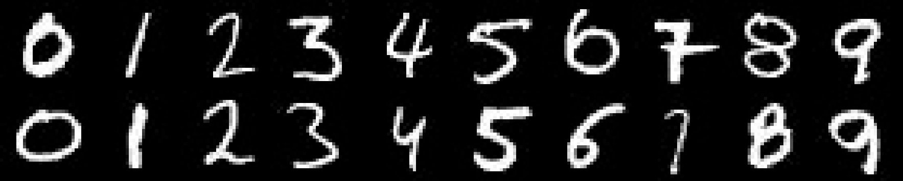 Figure 1
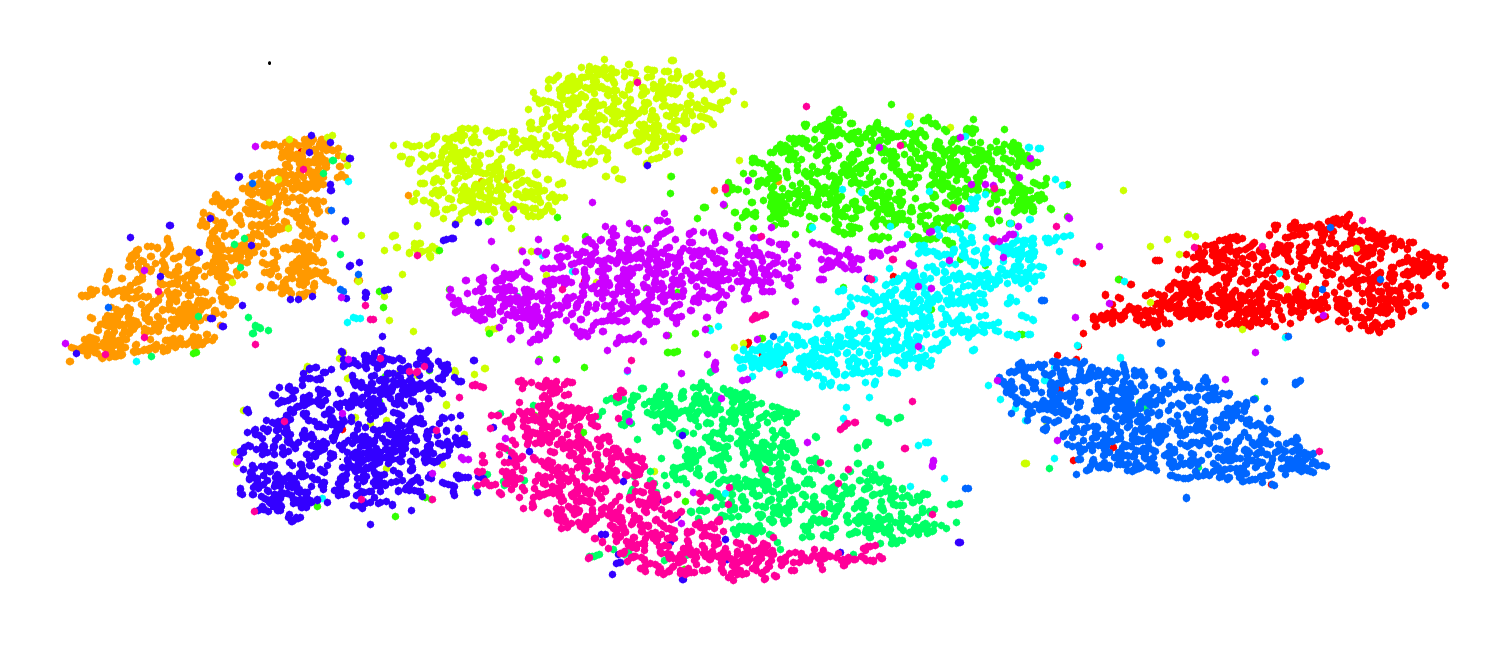 Figure 1
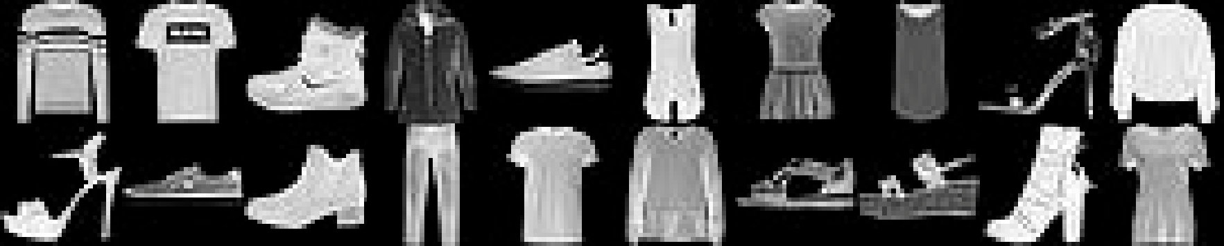 Figure 2
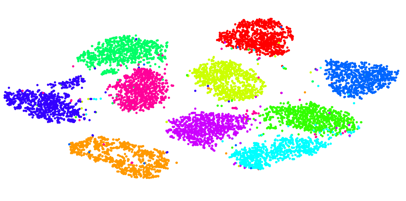 Figure 2
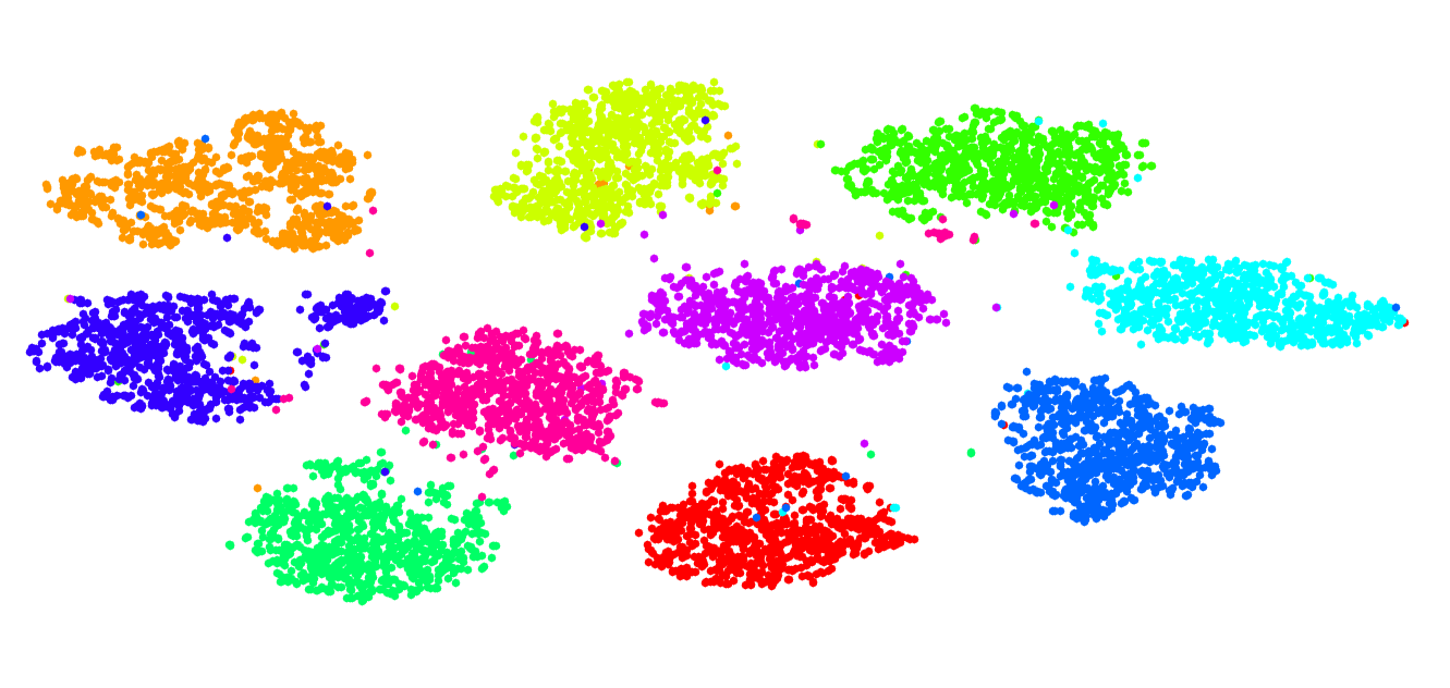 Figure 3
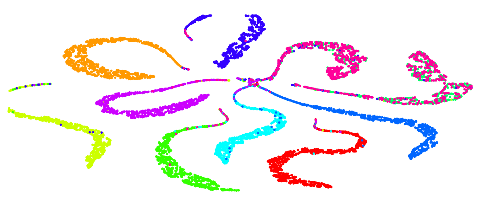 Figure 6
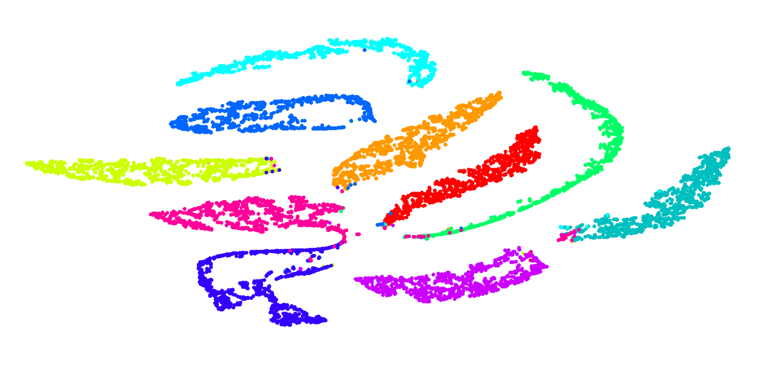 Figure 7
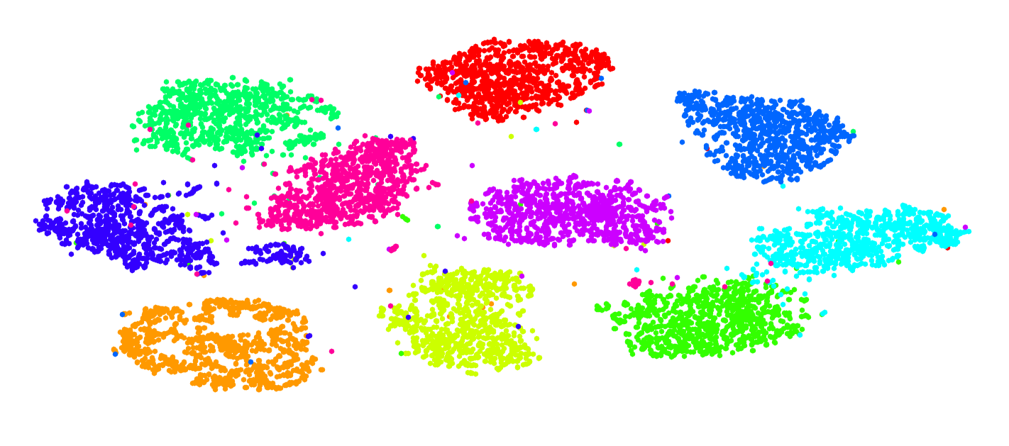 Figure 8
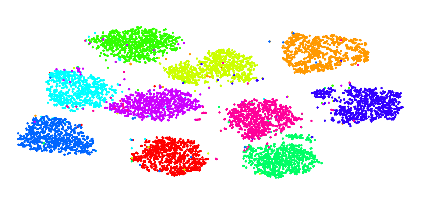 Figure 9
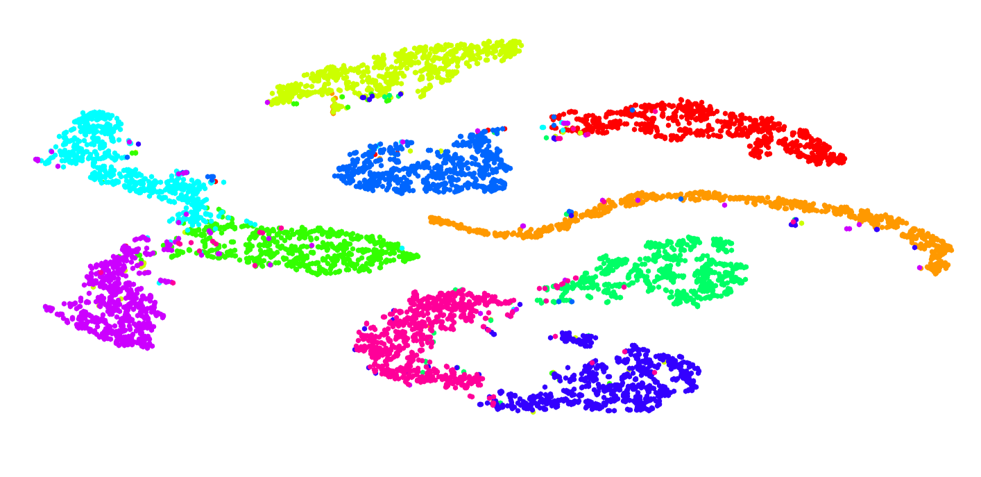 Figure 10
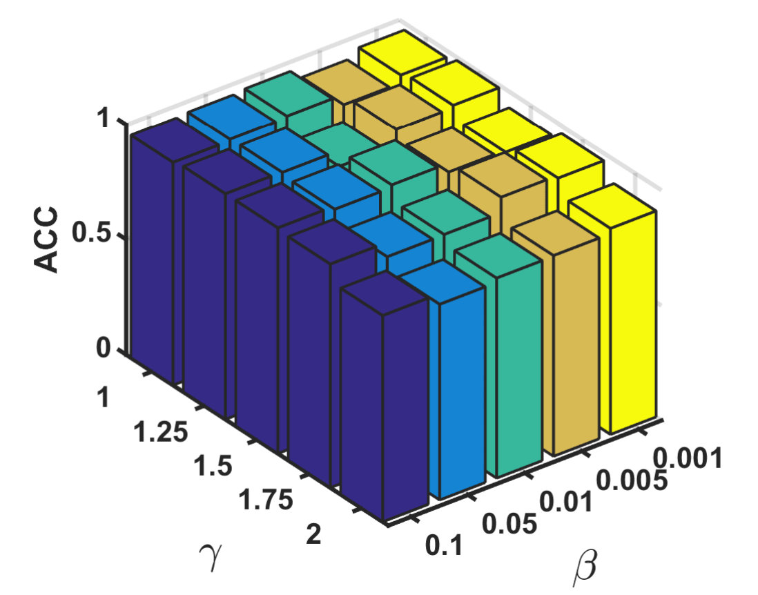 Figure 11
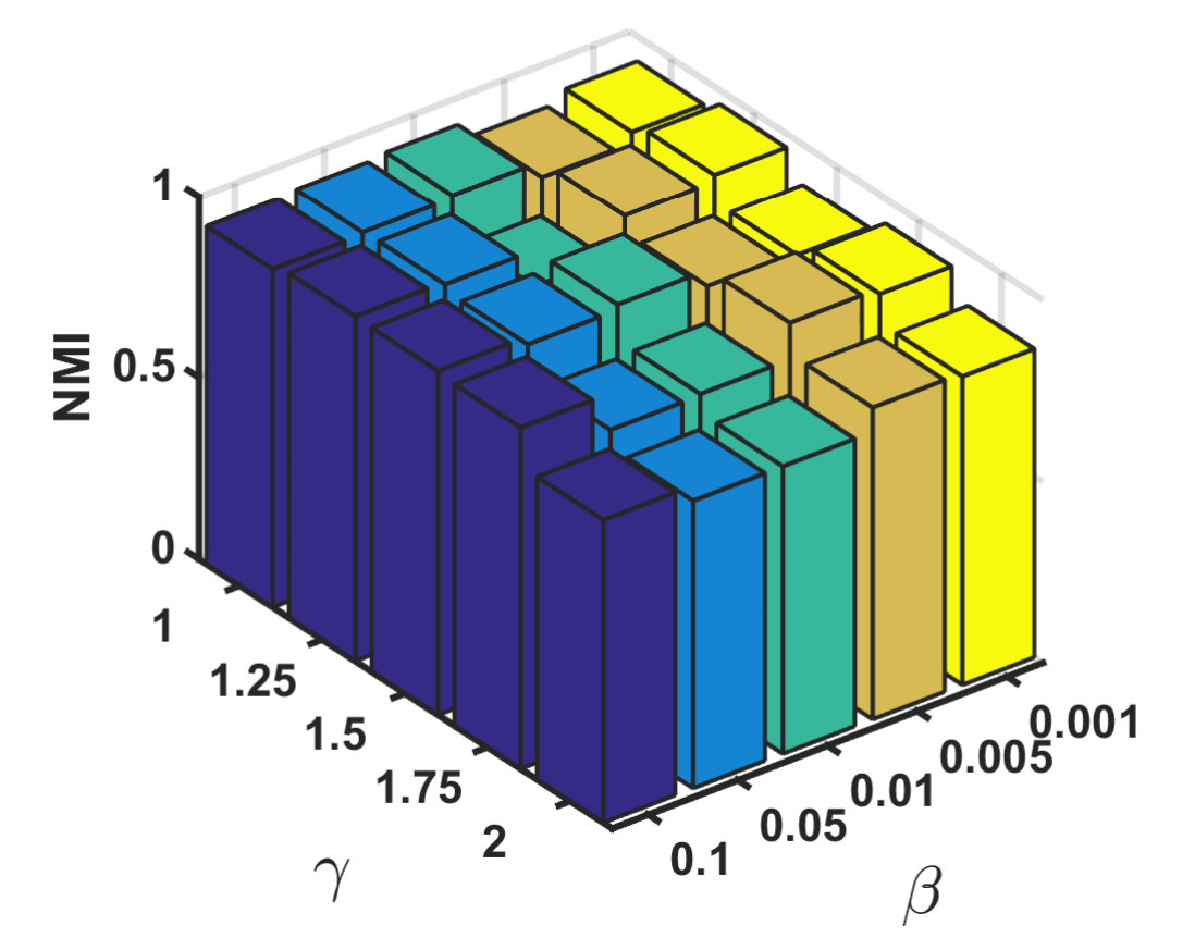 Figure 12
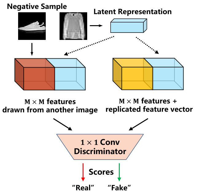 Figure 13
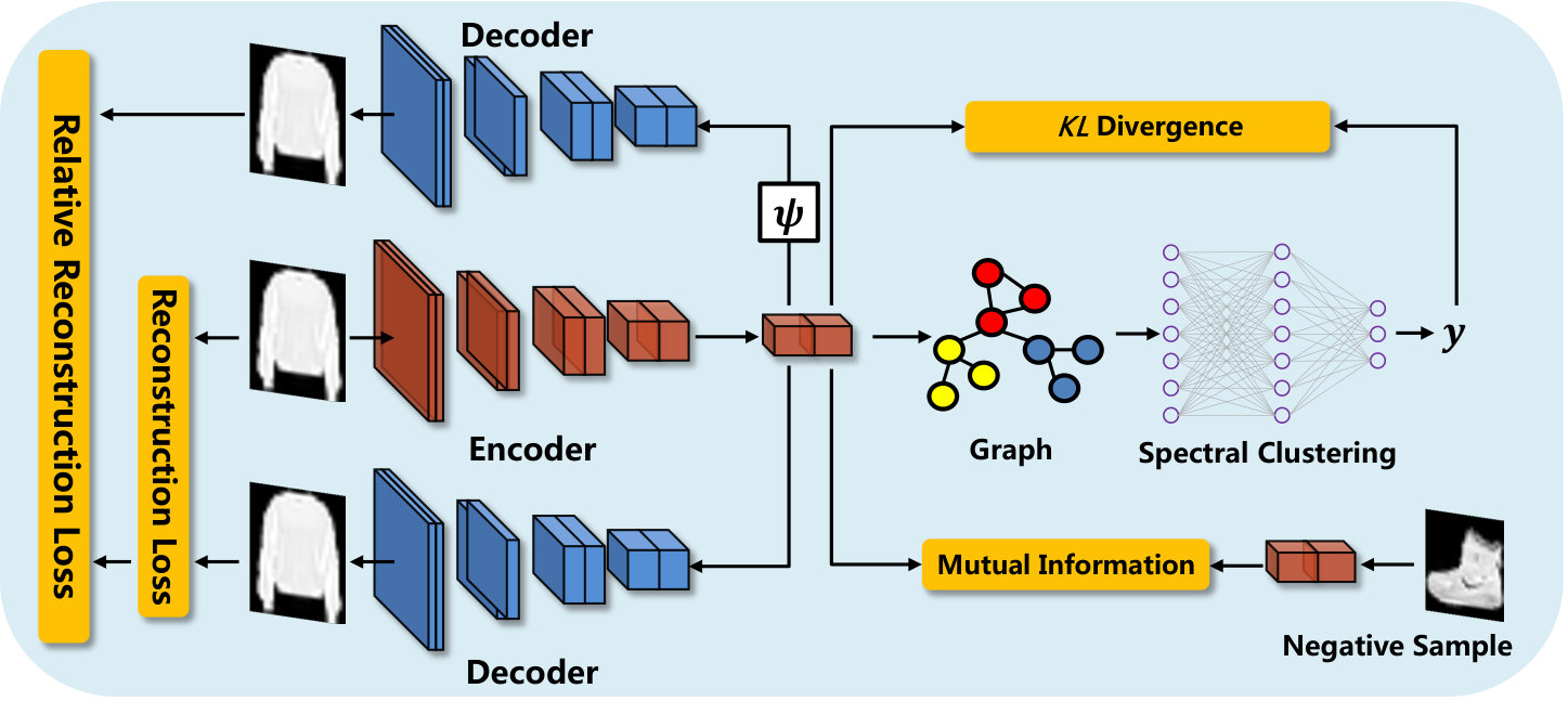 Figure 14
| Dataset | Samples | Classes | Dimensions |
|---|---|---|---|
| MNIST-full | 70,000 | 10 | 12828 |
| MNIST-test | 10,000 | 10 | 12828 |
| USPS | 9298 | 10 | 11616 |
| Fashion-Mnist | 70,000 | 10 | 12828 |
| YTF | 10,000 | 41 | 35555 |
| Method | encoder-1/decoder-4 | encoder-2/decoder-3 | encoder-3/decoder-2 | encoder-4/decoder-1 |
|---|---|---|---|---|
| MNIST | 3316 | 3316 | 3332 | 3332 |
| USPS | 3316 | 3332 | - | - |
| Fashion-Mnist | 3316 | 3316 | 3332 | 3332 |
| YTF | 5516 | 5516 | 5532 | 5532 |
| Method | MNIST-full | MNIST-test | USPS | Fashion-10 | YTF | |||||
| NMI | ACC | NMI | ACC | NMI | ACC | NMI | ACC | NMI | ACC | |
| K-means [28] | 0.500 | 0.532 | 0.501 | 0.546 | 0.601 | 0.668 | 0.512 | 0.474 | 0.776 | 0.601 |
| SC-Ncut [37] | 0.731 | 0.656 | 0.704 | 0.660 | 0.794 | 0.649 | 0.575 | 0.508 | 0.701 | 0.510 |
| SC-LS [4] | 0.706 | 0.714 | 0.756 | 0.740 | 0.755 | 0.746 | 0.497 | 0.496 | 0.759 | 0.544 |
| NMF [2] | 0.452 | 0.471 | 0.467 | 0.479 | 0.693 | 0.652 | 0.425 | 0.434 | - | - |
| AC-GDL [49] | 0.017 | 0.113 | 0.864 | 0.933 | 0.825 | 0.725 | 0.010 | 0.112 | 0.622 | 0.430 |
| DASC [50] | 0.784∗ | 0.801∗ | 0.780 | 0.804 | - | - | - | - | - | - |
| DEC [40] | 0.834∗ | 0.863∗ | 0.830∗ | 0.856∗ | 0.767∗ | 0.762∗ | 0.546∗ | 0.518∗ | 0.446∗ | 0.371∗ |
| VaDE [18] | 0.876 | 0.945 | - | - | 0.512 | 0.566 | 0.630 | 0.578 | - | - |
| JULE [44] | 0.913∗ | 0.964∗ | 0.915∗ | 0.961∗ | 0.913 | 0.950 | 0.608 | 0.563 | 0.848 | 0.684 |
| DEPICT [10] | 0.917∗ | 0.965∗ | 0.915∗ | 0.963∗ | 0.906 | 0.899 | 0.392 | 0.392 | 0.802 | 0.621 |
| IDEC [12] | 0.867∗ | 0.881∗ | 0.802 | 0.846 | 0.785∗ | 0.761∗ | 0.557 | 0.529 | - | - |
| SpectralNet [36] | 0.814 | 0.800 | 0.821 | 0.817 | - | - | - | - | 0.798 | 0.685 |
| InfoGAN [5] | 0.840 | 0.870 | - | - | - | - | 0.590 | 0.610 | - | - |
| ClusterGAN [30] | 0.890 | 0.950 | - | - | - | - | 0.640 | 0.630 | - | - |
| Our Method | 0.941 | 0.978 | 0.946 | 0.980 | 0.857 | 0.869 | 0.645 | 0.662 | 0.857 | 0.691 |
| Method | MNIST-full | MNIST-test | USPS | Fashion-10 | YTF | |||||
| NMI | ACC | NMI | ACC | NMI | ACC | NMI | ACC | NMI | ACC | |
| ConvAE | 0.745 | 0.776 | 0.751 | 0.781 | 0.652 | 0.698 | 0.556 | 0.546 | 0.642 | 0.476 |
| ConvAE+MI | 0.800 | 0.835 | 0.796 | 0.844 | 0.744 | 0.785 | 0.609 | 0.592 | 0.738 | 0.571 |
| ConvAE+RS | 0.803 | 0.841 | 0.801 | 0.850 | 0.752 | 0.798 | 0.597 | 0.614 | 0.721 | 0.558 |
| ConvAE+MI+RS | 0.910 | 0.957 | 0.914 | 0.961 | 0.827 | 0.831 | 0.640 | 0.656 | 0.801 | 0.606 |
| ConvAE+MI+RS+SN | 0.941 | 0.978 | 0.946 | 0.980 | 0.857 | 0.869 | 0.645 | 0.662 | 0.857 | 0.691 |
Peer Reviews
No public reviews on file for this paper yet. If you reviewed it on a platform where reviews are public (OpenReview, ICLR, NeurIPS, ICML), you can paste yours below so the community can read it here.
Videos
No videos yet. Explain this paper in a talk, walkthrough, or lecture? Add one.
Taxonomy
MethodsSpectral Clustering · Solana Customer Service Number +1-833-534-1729
Deep Spectral Clustering using Dual Autoencoder Network
Xu Yang1 , Cheng Deng1 , Feng Zheng2 , Junchi Yan3 , Wei Liu4*∗*
1School of Electronic Engineering, Xidian University, Xian 710071, China
2Department of Computer Science and Engineering, Southern University of Science and Technology
3Department of CSE, and MoE Key Lab of Artificial Intelligence, Shanghai Jiao Tong University
4Tencent AI Lab, Shenzhen, China
{xuyang.xd, chdeng.xd}@gmail.com, [email protected],
[email protected], [email protected] Corresponding author.
Abstract
The clustering methods have recently absorbed even-increasing attention in learning and vision. Deep clustering combines embedding and clustering together to obtain optimal embedding subspace for clustering, which can be more effective compared with conventional clustering methods. In this paper, we propose a joint learning framework for discriminative embedding and spectral clustering. We first devise a dual autoencoder network, which enforces the reconstruction constraint for the latent representations and their noisy versions, to embed the inputs into a latent space for clustering. As such the learned latent representations can be more robust to noise. Then the mutual information estimation is utilized to provide more discriminative information from the inputs. Furthermore, a deep spectral clustering method is applied to embed the latent representations into the eigenspace and subsequently clusters them, which can fully exploit the relationship between inputs to achieve optimal clustering results. Experimental results on benchmark datasets show that our method can significantly outperform state-of-the-art clustering approaches.
1 Introduction
As an important task in unsupervised learning [43, 8, 22, 24] and vision communities [48], clustering [14] has been widely used in image segmentation [37], image categorization [45, 47], and digital media analysis [1]. The goal of clustering is to find a partition in order to keep similar data points in the same cluster while dissimilar ones in different clusters. In recent years, many clustering methods have been proposed, such as -means clustering [28], spectral clustering [31, 46, 17], and non-negative matrix factorization clustering [41], among which -means and spectral clustering are two well-known conventional algorithms that are applicable to a wide range of various tasks. However, these shallow clustering methods depend on low-level features such as raw pixels, SIFT [32] or HOG [7] of the inputs. Their distance metrics are only exploited to describe local relationships in data space, and have limitation to represent the latent dependencies among the inputs [3].
This paper presents a novel deep learning based unsupervised clustering approach. Deep clustering, which integrates embedding and clustering processes to obtain optimal embedding subspace for clustering, can be more effective than shallow clustering methods. The main reason is that the deep clustering methods can effectively model the distribution of the inputs and capture the non-linear property, being more suitable to real-world clustering scenarios.
Recently, many clustering methods are promoted by deep generative approaches, such as autoencoder network [29]. The popularity of the autoencoder network lies in its powerful ability to capture high dimensional probability distributions of the inputs without supervised information. The encoder model projects the inputs into the latent space, and adopts an explicit approximation of maximum likelihood to estimate the distribution diversity between the latent representations and the inputs. Simultaneously, the decoder model reconstructs the latent representations to ensure the output maintaining all of the details in the inputs [38]. Almost all existing deep clustering methods endeavor to minimize the reconstruction loss. The hope is making the latent representations more discriminative which directly determines the clustering quality. However, in fact, the discriminative ability of the latent representations has no substantial connection with the reconstruction loss, causing the performance gap that is to be bridged in this paper.
We propose a novel dual autoencoder network for deep spectral clustering. First, a dual autoencoder, which enforces the reconstruction constraint for the latent representations and their noisy versions, is utilized to establish the relationships between the inputs and their latent representations. Such a mechanism is performed to make the latent representations more robust. In addition, we adopt the mutual information estimation to reserve discriminative information from the inputs to an extreme. In this way, the decoder can be viewed as a discriminator to determine whether the latent representations are discriminative. Fig. 1 demonstrates the performance of our proposed autoencoder network by comparing different data representations on MNIST-test data points. Obviously, our method can provide more discriminative embedding subspace than the convolution autoencoder network. Furthermore, deep spectral clustering is harnessed to embed the latent representations into the eigenspace, which followed by clustering. This procedure can exploit the relationships between the data points effectively and obtain the optimal results. The proposed dual autoencoder network and deep spectral clustering network are jointly optimized.
The main contributions of this paper are in three-folds:
- •
We propose a novel dual autoencoder network for generating discriminative and robust latent representations, which is trained with the mutual information estimation and different reconstruction results.
- •
We present a joint learning framework to embed the inputs into a discriminative latent space with a dual autoencoder and assign them to the ideal distribution by a deep spectral clustering model simultaneously.
- •
Empirical experiments demonstrate that our method outperforms state-of-the-art methods over the five benchmark datasets, including both traditional and deep network-based models.
2 Related Work
Recently, a number of deep learning-based clustering methods are proposed. Deep Embedding Clustering [40] (DEC) adopts a fully connected stacked autoencoder network in order to learn the latent representations by minimizing the reconstruction loss in the pre-training phase. The objective function applied to the clustering phase is the Kullback Leibler () divergence between the soft assignments of clustering modelled by a -distribution. And then, a -means loss is adopted at the clustering phase to train a fully connected autoencoder network [42], which is a joint approach of dimensionality reduction and -means clustering. In addition, Gaussian Mixture Variational Autoencoder (GMVAE) [9] shows that minimum information constraint can be utilized to mitigate the effect of over-regularization in VAEs and provides an unsupervised clustering within the VAE framework considering a Gaussian mixture as a prior distribution. Discriminatively Boosted Clustering [23], a fully convolutional network with layer-wised batch normalization, adopts the same objective function as DEC and uses a boosting factor to the relatively train a stacked autoencoder.
Shah and Koltun [34] jointly solve the tasks of clustering and dimensionality reduction by efficiently optimizing a continuous global objective based on robust statistics, which allows heavily mixed clusters to be untangled. Following this method, a deep continuous clustering approach is suggested in [35], where the autoencoder parameters and a set of representatives defined against each data-point are simultaneously optimized. The convex clustering approach proposed by [6] optimizes the representatives by minimizing the distances between each representative and its associated data-point. Non-convex objectives are involved to penalize for the pairwise distances between the representatives.
Furthermore, to improve the performance of clustering, some methods combine convolutional layers with fully connected layers. Joint Unsupervised Learning (JULE) [44] jointly optimizes a convolutional neural network with the clustering parameters in a recurrent manner using an agglomerative clustering approach, where image clustering is conducted in the forward pass and representation learning is performed in the backward pass. Dizaji [10] proposes DEPICT, a method that trains a convolutional auto-encoder with a softmax layer stacked on-top of the encoder. The softmax entries represent the assignment of each data-point to one cluster. VaDE [18] is a variational autoencoder method for deep embedding, and combines a Gaussian Mixture Model for clusering. In [16], a deep autoencoder is trained to minimize a reconstruction loss together with a self-expressive layer. This objective encourages a sparse representation of the original data. Zhou et al. [50] presents a deep adversarial subspace clustering (DASC) method to learn more favorable representations and supervise sample representation learning by adversarial deep learning [21]. However, the results of reconstruction through low-dimensional representations are often very blurry. One possible way is to train a discriminator with adversarial learning but it can further increase the difficulty of training. Comparatively, our method introduces a relative reconstruction loss and mutual information estimation to obtain more discriminative representations, and jointly optimize the autoencoder network and the deep spectral clustering network for optimal clustering.
3 Methodology
As aforementioned, our framework consists of two main components: a dual autoencoder and a deep spectral clustering network. The dual autoencoder, which reconstructs the inputs using the latent representations and their noise versions, is introduced to make the latent representations more robust. In addition, the mutual information estimation between the inputs and the latent representations is applied to preserve the input information as much as possible. Then we utilize the deep spectral clustering network to embed the latent representations into the eigenspace and subsequently clustering is performed. The two networks are merged into a unified framework and jointly optimized with divergence. The framework is shown in Fig. 2.
Let denote the input samples, denote their corresponding latent representations where is learned by the encoder . The parameters of the encoder are defined by , and is the feature dimension. represents the reconstructed data point, which is the output of the decoder , and the parameters of the decoder are denoted by . We adopt a deep spectral clustering network to map to , where is the number of clusters.
3.1 Discriminative latent representation
We first train the dual autoencoder network to embed the inputs into a latent space. Based on the original reconstruction loss, we add a noise-disturbed reconstruction loss to learn the decoder network. In addition, we introduce the maximization of mutual information [13] to the learning procedure of the encoder network, so that the network can obtain more robust representations.
Encoder: Feature extraction is the major step in clustering and a good feature can effectively improve clustering performance. However, a single reconstruction loss cannot well guarantee the quality of the latent representations. We hope that the representations will help us to identify the sample from the inputs, which means it is the most unique information extracted from the inputs. Mutual information measures the essential correlation between two samples and can effectively estimate the similarity between features and inputs . The definition of mutual information is defined as:
[TABLE]
where is the distribution of the inputs, is the distribution of the latent representations, and the distribution of latent space can be calculated by . The mutual information is expected to be as large as possible when training the encoder network, hence we have:
[TABLE]
In addition, the learned latent representations are required to obey the prior distribution of the standard normal distribution with divergence. This is beneficial to make the latent space more regular. The distribution difference between and its prior is defined as.
[TABLE]
According to Eqs. (2) and (3), we have:
[TABLE]
It can be further rewritten as:
[TABLE]
According to Eq. (1), the Eq. (5) can be viewed as:
[TABLE]
Unfortunately, divergence is unbounded. Instead of using divergence, divergence is adopted for mutual information maximization:
[TABLE]
We have known that the variational estimation of divergence [33] is defined as:
[TABLE]
where [33]. Here and are utilized to replace and . As a result, Eq. (7) can be defined as:
[TABLE]
Negative sampling estimation [13], which is the process of using a discriminator to distinguish the real and noisy samples to estimate the distribution of real samples, is generally utilized to solve the problem in Eq. (9). is a discriminator, where and its latent representation together form a positive sample pair. We randomly select from the disturbed batch to construct a negative sample pair according to . Note that Eq. (9) represents the global mutual information between and .
Furthermore, we extract the feature map from the middle layer of the convolutional network, and construct the relationship between the feature map and the latent representation, which is the local mutual information. The estimation method plays the same role as global mutual information. The middle layer feature are combined with the latent representation to obtain a new feature map. Then a convolution is considered as the estimation network of local mutual information, as shown in Fig. 3. The selection method of negative samples is the same as global mutual information estimation. Therefore, the objective function that needs to be optimized can be defined as:
[TABLE]
where and represent the height and width of the feature map. represents the feature vector of the middle feature map at coordinates and is the standard normal distribution.
Decoder: In the existing decoder networks, the reconstruction loss is generally a suboptimal scheme for clustering, due to the natural trade-off between the reconstruction and the clustering tasks. The reconstruction loss mainly depends on the two parts: the distribution of the latent representations and the generative capacity of decoder network. However, the generative capacity of the decoder network is not required in the clustering task. Our real goal is not to obtain the best reconstruction results, but to get more discriminative features for clustering. We directly use noise disturbance in the latent space to discard known nuisance factors from the latent representations. Models trained in this fashion become robust by exclusion rather than inclusion, and are expected to perform well on clustering tasks, where even the inputs contain unseen nuisance [15]. A noisy-transformer is utilized to convert the latent representations into their noisy versions , and then the decoder reconstructs the inputs from and . The reconstruction results can be defined as and , and the relative reconstruction loss can be written as:
[TABLE]
where stands for the Frobenius norm. We also use the original reconstruction loss to ensure the performance of the decoder network and consider as multiplicative Gaussian noise. The complete reconstruction loss can be defined as:
[TABLE]
where stands for the strength of different reconstruction loss.
Hence, by considering all the items, the total loss of the autoencoder network can be defined as:
[TABLE]
3.2 Deep Spectral Clustering
The learned autoencoder parameters and are considered as an initial condition in the clustering phase. Spectral clustering can effectively use the relationship between samples to reduce intra-class differences, and produce better clustering results than -means. In this step, we first adopt the autoencoder network to learn the latent representations. Next, a spectral clustering method is used to embed the latent representations into the eigenspace of their associated graph Laplacian matrix [25]. All the samples will be subsequently clustered in this space. Finally, both the autoencoder parameters and clustering objective are jointly optimized.
Specifically, we first utilize the latent representations to construct the non-negative affinity matrix :
[TABLE]
The loss function of spectral clustering is defined as:
[TABLE]
where is the output of the network. When we adopt the general neural network to output , we randomly select a minibatch of samples at each iteration and thus the loss function can be defined as:
[TABLE]
In order to prevent that all points are grouped into the same cluster in network maps, the output is required to be orthonormal in expectation. That is to say:
[TABLE]
where is a matrix of the outputs whose th row is . The last layer of the network is utilized to enforce the orthogonality [36] constraint. This layer gets input from units, and acts as a linear layer with outputs, in which the weights are required to be orthogonal, producing the orthogonalized output for a minibatch. Let denote the matrix containing the inputs to this layer for , a linear map that orthogonalizes the columns of is computed through its QR decomposition. Since integrated is full rank for any matrix , the QR decomposition can be obtained by the Cholesky decomposition:
[TABLE]
where is a lower triangular matrix, and . Therefore, in order to orthogonalize , the last layer multiplies from the right by . Actually, can be obtained from the Cholesky decomposition of and the factor is needed to satisfy Eq. (17).
We unify the latent representation learning and the spectral clustering using divergence. In the clustering phase, the last term of Eq. (10) can be rewritten as:
[TABLE]
where and . Note is a normal distribution with mean and variance . Therefore, the overall loss of the autoencoder and the spectral clustering network is defined as:
[TABLE]
Finally, we jointly optimize the two networks until convergence to obtain the desired clustering results.
4 Experiments
In this section, we evaluate the effectiveness of the proposed clustering method in five benchmark datasets, and then compare the performance with several state-of-the-arts.
4.1 Datasets
In order to show that our method works well with various kinds of datasets, we choose the following image datasets. Considering that clustering tasks are fully unsupervised, we concatenate the training and testing samples when applicable. MNIST-full [20]: A dataset containing a total of 70,000 handwritten digits with 60,000 training and 10,000 testing samples, each being a 3232 monochrome image. MNIST-test: A dataset only consists of the testing part of MNIST-full data. USPS: A handwritten digits dataset from the USPS postal service, containing 9,298 samples of 1616 images. Fashion-MNIST [39]: This dataset has the same number of images and the same image size with MNIST, but it is fairly more complicated. Instead of digits, it consists of various types of fashion products. YTF: We adopt the first 41 subjects of YTF dataset and the images are first cropped and resized to . Some image samples are shown in Fig. 4. The brief descriptions of the datasets are given in Tab. 1.
4.2 Clustering Metrics
To evaluate the clustering results, we adopt two standard evaluation metrics: Accuracy (ACC) and Normalized Mutual Information (NMI) [41].
The best mapping between cluster assignments and true labels is computed using the Hungarian algorithm to measure accuracy [19]. For completeness, we define ACC by:
[TABLE]
where and are the true label and predicted cluster of data point .
NMI calculates the normalized measure of similarity between two labels of the same data, which is defined as:
[TABLE]
where denotes the mutual information between true label and predicted cluster , and represents their entropy. Results of NMI do not change by permutations of clusters (classes), and they are normalized to the range of [0, 1], with 0 meaning no correlation and 1 exhibiting perfect correlation.
4.3 Implementation Details
In our experiments, we set , , and . The channel numbers and kernel sizes of the autoencoder network are shown in Tab. 2, and the dimension of latent space is set to 120. The deep spectral clustering network consists of four fully connected layers, and we adopt ReLU [26] as the non-linear activations. We construct the original weight matrix with probabilistic -nearest neighbors for each dataset. The weight is calculated as nearest-neighbor graph [11], and the number of neighbors is set to 3.
4.4 Comparison Methods
We compare our clustering model with several baselines, including -means [28], spectral clustering with normalized cuts (SC-Ncut) [37], large-scale spectral clustering (SC-LS) [4], NMF [2], graph degree linkage-based agglomerative clustering (AC-GDL) [49]. In addition, we also evaluate the performance of our method with several state-of-the-art clustering algorithms based on deep learning, including deep adversarial subspace clustering (DASC) [50], deep embedded clustering (DEC) [40], variational deep embedding (VaDE) [18], joint unsupervised learning (JULE) [44], deep embedded regularized clustering (DEPICT) [10], improved deep embedded clustering with locality preservation (IDEC) [12], deep spectral clustering with a set of nearest neighbor pairs (SpectralNet) [36], clustering with GAN (ClusterGAN) [30] and GAN with the mutual information (InfoGAN) [5].
4.5 Evaluation of Clustering Algorithm
We run our method with 10 random trials and report the average performance, the error range is no more than 2%. In terms of the compared methods, if the results of their methods on some datasets are not reported, we run the released code with hyper-parameters mentioned in their papers, and the results are marked by (*) on top. When the code is not publicly available, or running the released code is not practical, we put dash marks (-) instead of the corresponding results.
The clustering results are shown in Tab. 3, where the first five are conventional clustering methods. In the table, we can notice that our proposed method outperforms the competing methods on these benchmark datasets. We observe that the proposed method can improve the clustering performance whether in digital datasets or in other product dataset. Especially when performing on the object dataset MNIST-test, the clustering accuracy is over 98%. Specifically, it exceeds the second best DEPICT which is trained on the noisy versions of the inputs by 1.6% and 3.1% on ACC and NMI respectively. Moreover, our method achieves much better clustering results than several classical shallow baselines. This is because compared with shallow methods, our method uses a multi-layer convolutional autoencoder as the feature extractor and adopts deep clustering network to obtain the most optimal clustering results. The Fashion-MNIST dataset is very difficult to deal with due to the complexity of samples, but our method still harvests good results.
We also investigate the parameter sensitivity on MNIST-test, and the results are shown in Fig. 5, where Fig. 5 represents the results of ACC from different parameters and Fig. 5 is the results of NMI. It intuitively demonstrates that our method maintains acceptable results with most parameter combinations and has relative stability.
4.6 Evaluation of Learning Approach
We compare different strategies for training our model. For training a multi-layer convolutional autoencoder, we analyze the following four approaches: (1) convolutional autoencoder with original reconstruction loss (ConvAE), (2) convolutional autoencoder with original reconstruction loss and mutual information (ConvAE+MI), (3) convolutional autoencoder with improved reconstruction loss (ConvAE+RS) and (4) convolutional autoencoder with improved reconstruction loss and mutual information (ConvAE+MI+RS). The last one is the joint training of convolutional autoencoder and deep spectral clustering. Tab. 4 represents the performance of different strategies for training our model. It clearly demonstrates that each kind of strategy of our method can improve the accuracy of clustering effectively, especially after adding mutual information and the improved reconstruction loss in the convolutional autoencoder network. Fig. 6 demonstrates the importance of our proposed strategy by comparing different data representations of MNIST-test data points using -SNE visualization [27], Fig. 6(a) represents the space of raw data, Fig. 6(b) is the data points in the latent subspace of convolution autoencoder, Fig. 6(c) and 6(d) are the results of DEC and SpectralNet respectively, and the rest are our proposed model with different strategies. The results demonstrate the latent representations obtained by our method have more clear distribution structure.
5 Conclusion
In this paper, we propose an unsupervised deep clustering method with a dual autoencoder network and a deep spectral network. First, the dual autoencoder, which reconstructs the inputs using the latent representations and their noise-contaminated versions, is utilized to establish the relationships between the inputs and the latent representations in order to obtain more robust latent representations. Furthermore, we maximize the mutual information between the inputs and the latent representations, which can preserve the information of the inputs as much as possible. Hence, the features of the latent space obtained by our autoencoder are robust to noise and more discriminative. Finally, the spectral network is fused to a unified framework to cluster the features of the latent space, so that the relationship between the samples can be effectively utilized. We evaluate our method on several benchmarks and experimental results show that our method outperforms those state-of-the-art approaches.
6 Acknowledgement
Our work was also supported by the National Natural Science Foundation of China under Grant 61572388, 61703327 and 61602176, the Key R&D Program-The Key Industry Innovation Chain of Shaanxi under Grant 2017ZDCXL-GY-05-04-02, 2017ZDCXL-GY-05-02 and 2018ZDXM-GY-176, and the National Key R&D Program of China under Grant 2017YFE0104100.
The reference list from the paper itself. Each links out to its DOI / PubMed record.
- 1[1] Lingling An, Xinbo Gao, Xuelong Li, Dacheng Tao, Cheng Deng, Jie Li, et al. Robust reversible watermarking via clustering and enhanced pixel-wise masking. IEEE Trans. Image Processing , 21(8):3598–3611, 2012.
- 2[2] Deng Cai, Xiaofei He, Xuanhui Wang, Hujun Bao, and Jiawei Han. Locality preserving nonnegative matrix factorization. In IJCAI , volume 9, pages 1010–1015, 2009.
- 3[3] Pu Chen, Xinyi Xu, and Cheng Deng. Deep view-aware metric learning for person re-identification. In IJCAI , pages 620–626, 2018.
- 4[4] Xinlei Chen and Deng Cai. Large scale spectral clustering with landmark-based representation. In AAAI , volume 5, page 14, 2011.
- 5[5] Xi Chen, Yan Duan, Rein Houthooft, John Schulman, Ilya Sutskever, and Pieter Abbeel. Infogan: Interpretable representation learning by information maximizing generative adversarial nets. In Advances in neural information processing systems , pages 2172–2180, 2016.
- 6[6] Eric C Chi and Kenneth Lange. Splitting methods for convex clustering. Journal of Computational and Graphical Statistics , 24(4):994–1013, 2015.
- 7[7] Navneet Dalal and Bill Triggs. Histograms of oriented gradients for human detection. In Computer Vision and Pattern Recognition, 2005. CVPR 2005. IEEE Computer Society Conference on , volume 1, pages 886–893. IEEE, 2005.
- 8[8] C Deng, E Yang, T Liu, W Liu, J Li, and D Tao. Unsupervised semantic-preserving adversarial hashing for image search. IEEE transactions on image processing: a publication of the IEEE Signal Processing Society , 2019.