Improved bounds for the excluded-minor approximation of treedepth
Wojciech Czerwi\'nski, Wojciech Nadara, Marcin Pilipczuk

TL;DR
This paper establishes improved bounds relating treedepth and treewidth, providing new structural insights and algorithms for approximating treedepth in graphs, with implications for sparse graph theory.
Contribution
It introduces tighter bounds connecting treedepth and treewidth, and offers polynomial-time algorithms for treedepth approximation with better guarantees than previous results.
Findings
Bound of treedepth $ o$ either large treewidth or specific subgraphs
Improved bound from $ ilde{ ext{Omega}}(k^5)$ to $ ext{Omega}(k^3)$ for treedepth
Polynomial-time algorithm for treedepth approximation with improved factor
Abstract
Treedepth, a more restrictive graph width parameter than treewidth and pathwidth, plays a major role in the theory of sparse graph classes. We show that there exists a constant such that for every positive integers and a graph , if the treedepth of is at least , then the treewidth of is at least or contains a subcubic (i.e., of maximum degree at most ) tree of treedepth at least as a subgraph. As a direct corollary, we obtain that every graph of treedepth is either of treewidth at least , contains a subdivision of full binary tree of depth , or contains a path of length . This improves the bound of of Kawarabayashi and Rossman [SODA 2018]. We also show an application of our techniques for approximation algorithms of treedepth: given a graph of treedepth and treewidth , one can in…
Click any figure to enlarge with its caption.
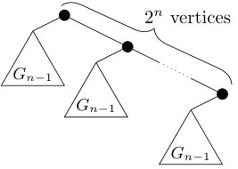 Figure 1
Peer Reviews
No public reviews on file for this paper yet. If you reviewed it on a platform where reviews are public (OpenReview, ICLR, NeurIPS, ICML), you can paste yours below so the community can read it here.
Videos
No videos yet. Explain this paper in a talk, walkthrough, or lecture? Add one.
Improved bounds for the excluded-minor approximation of treedepth††thanks: This research is a part of a project that have received funding from the European Research Council (ERC)
under the European Union’s Horizon 2020 research and innovation programme Grant Agreement 714704. An extented abstract of this work appeared at ESA 2019 [2].
Wojciech Czerwiński111University of Warsaw, Poland, [email protected]
Wojciech Nadara222University of Warsaw, Poland, [email protected]
Marcin Pilipczuk333University of Warsaw, Poland, [email protected]
Abstract
Treedepth, a more restrictive graph width parameter than treewidth and pathwidth, plays a major role in the theory of sparse graph classes. We show that there exists a constant such that for every positive integers and a graph , if the treedepth of is at least , then the treewidth of is at least or contains a subcubic (i.e., of maximum degree at most ) tree of treedepth at least as a subgraph.
As a direct corollary, we obtain that every graph of treedepth is either of treewidth at least , contains a subdivision of full binary tree of depth , or contains a path of length . This improves the bound of of Kawarabayashi and Rossman [SODA 2018].
We also show an application of our techniques for approximation algorithms of treedepth: given a graph of treedepth and treewidth , one can in polynomial time compute a treedepth decomposition of of width . This improves upon a bound of stemming from a tradeoff between known results.
The main technical ingredient in our result is a proof that every tree of treedepth contains a subcubic subtree of treedepth at least .
{textblock}
20(0, 12.4)
{textblock}20(0, 13.4)
1 Introduction
For an undirected graph , the treedepth of is the minimum height of a rooted forest whose ancestor-descendant closure contains as a subgraph. Together with more widely known related width notions such as treewidth and pathwidth, it plays a major role in structural graph theory, in particular in the study of general sparse graph classes [10, 9, 8].
An important property of treedepth is that it admits a number of equivalent definitions. Following the definition of treedepth above, a treedepth decomposition of a graph consists of a rooted forest and an injective mapping such that for every the vertices and are in ancestor-descendant relation in . The width of a treedepth decomposition is the height of (the number of vertices on the longest leaf-to-root path in ) and the treedepth of is the minimum possible height of a treedepth decomposition of . A centered coloring of a graph is an assignment such that for every connected subgraph of , has a center in : a vertex of unique color, i.e., for every . A vertex ranking of a graph is an assignment such that in every connected subgraph of there is a unique vertex of maximum rank (value ). Clearly, each vertex ranking is a centered coloring. It turns out that the minimum number of colors (minimum size of the image of ) needed for a centered coloring and for a vertex ranking are equal and equal to the treedepth of a graph [8].
While there are multiple examples of algorithmic usage of treedepth in the theory of sparse graphs [9, 10], our understanding of the complexity of computing minimum width treedepth decompositions is limited. For a graph , let and denote the treedepth and the treewidth of , respectively. An algorithm of Reidl, Rossmanith, Villaamil, and Sikdar [11] computes exactly the treedepth of an input graph in time , given a tree decomposition of of width . Combined with the classic constant-factor approximation algorithm for treewidth that runs in time [12], one obtains an exact algorithm for treedepth running in time . No faster exact algorithm is known.
For approximation algorithms, the following folklore lemma (presented with full proof in [6]) is very useful.
Lemma 1.1**.**
Given a graph and a tree decomposition of of maximum bag size , one can in polynomial time compute a treedepth decomposition of of width at most .
Using Lemma 1.1, one can obtain an approximation algorithm for treedepth with a cheap tradeoff trick.444This trick has been observed and communicated to us by Michał Pilipczuk. We thank Michał for allowing us to include it in this paper.
Lemma 1.2**.**
Given a graph , one can in polynomial time compute a treedepth decomposition of of width .
Proof.
Let . Using the polynomial-time approximation algorithm for treewidth [5], compute a tree decomposition of of width and bags. For every integer , use the algorithm of [11] to check in polynomial time if the treedepth of is at most . Note that if this is the case, the algorithm finds an optimal treedepth decomposition and we can conclude. Otherwise, we have and we apply Lemma 1.1 to and obtaining a treedepth decomposition of of width
[TABLE]
∎
Lemma 1.2 is the only polynomial approximation algorithm for treedepth running in polynomial time we are aware of.
A related topic to exact and approximation algorithms computing minimum-width treedepth decomposition is the study of obstructions to small treedepth. Dvořák, Giannopoulou, and Thilikos [4] proved that every minimal graph of treedepth has the number of vertices at most double-exponential in . More recently, Kawarabayashi and Rossman showed an excluded-minor theorem for treedepth.
Theorem 1.3** ([6]).**
There exists a universal constant such that for every integer every graph of treedepth at least is either of treewidth at least , contains a subdivision of a full binary tree of depth as a subgraph, or contains a path of length .
While neither the results of [4] nor [6] have a direct application in the approximability of treedepth, these topics are tightly linked with each other and we expect that a finer understanding of treedepth obstructions is necessary to provide more efficient algorithms computing or approximating the treedepth of a graph.
Our results.
Our main graph-theoretical result is the following statement, improving upon the work of Kawarabayashi and Rossman [6].
Theorem 1.4**.**
Let be a graph of treewidth and treedepth . Then there exists a subcubic tree that is a subgraph of and is of treedepth at least
[TABLE]
In other words, Theorem 1.4 states that there exists a constant such that for every graph and positive integers , if the treedepth of is at least , then the treewidth of is at least or contains a subcubic tree of treedepth . Since every subcubic tree of treedepth contains either a simple path of length or a subdivision of a full binary tree of depth [6], we have the following corollary.
Corollary 1.5**.**
Let be a graph of treewidth and treedepth . Then for some
[TABLE]
* contains either a simple path of length or a subdivision of a full binary tree of depth .*
Consequently, there exists an absolute constant such that for every integer and a graph of treedepth at least , either
- •
* has treewidth at least ,*
- •
* contains a subdivision of a full binary tree of depth as a subgraph, or*
- •
* contains a path of length .*
In other words, Corollary 1.5 improves the bound of Kawarabayashi and Rossman [6] to . We remark here that there are subcubic trees of treedepth that contains neither a path of length nor a subdivision of a full binary tree of depth ,555It is straightforward to deduce such an example from the proof of [6]. We provide such an example in Section 7. and thus the quadratic loss between the statements of Theorem 1.4 and Corollary 1.5 is necessary.
Inside the proof of Theorem 1.4 we make use of the following lemma that may be of independent interest. This lemma is the main technical improvement upon the work of Kawarabayashi and Rossman [6].
Lemma 1.6**.**
*Every tree of treedepth contains a subcubic subtree of treedepth at least .
Furthermore, such a subtree can be found in polynomial time.*
Lemma 1.6, developed to prove Theorem 1.4, have some implications on the approximability of treedepth. We combine it with the machinery of Kawarabayashi and Rossman [6] to improve upon Lemma 1.2 as follows.
Theorem 1.7**.**
Given a graph , one can in polynomial time compute a treedepth decomposition of of width .
The result of Kawarabayashi and Rossman [6] has been also an important ingredient in the study of linear colorings [7]. A coloring of a graph is a linear coloring if for every (not necessarily induced) path in there exists a vertex of unique color on . Clearly, each centered coloring is a linear coloring, but the minimum number of colors needed for a linear coloring can be much smaller than the treedepth of a graph. Kun et al. [7] provided a polynomial relation between the treedepth and the minimum number of colors in a linear coloring; by replacing their usage of [6] by our result (and using an improved bound for the excluded grid theorem [1]) we obtain an improved bound.
Theorem 1.8**.**
There exists a polynomial such that for every integer and graph , if the treedepth of is at least , then every linear coloring of requires at least colors.
The previous bound of [7] is .
Brief preliminaries on tree decompositions, treewidth, and brambles can be found in Section 2. After proving Lemma 1.6 in Section 3, we prove Theorem 1.4 in Section 4.
Then in Section 5 we provide a proof a lemma that combines the machinery of Kawarabayashi and Rossman [6] with Lemma 1.6 and conclude the proof of Theorem 1.7 using it. Finally, Theorem 1.8 is proven in Section 6.
2 Preliminaries
The symbol stands for base- logarithm and stands for . We denote ; note that is chosen in a way so that and .
We need a few basic notions concerning tree decompositions and treewidth. Recall that a tree decomposition of a graph is a pair where is a rooted tree and is such that for every the set induces a connected nonempty subtree of and for every there exists with . The width of a tree decomposition is and the treewidth of a graph is the minimum possible width of its tree decomposition.
A bramble in a graph is a family of connected subgraphs of such that for every , either and share a vertex or there is an edge of with one endpoint in and one endpoint in . Standard arguments (see e.g. [3]) show the following:
Lemma 2.1**.**
Let be a graph, be a tree decomposition of , and let be a bramble in . Then there exists such that for every it holds that .
3 Subcubic subtrees of trees of large treedepth
This section focuses on proving Lemma 1.6.
Schäffer [13] proved that there is a linear time algorithm for finding a vertex ranking with minimum number of colors of a tree . We follow [7] for a good description of its properties.
In original Schäffer’s algorithm ranks are starting from , however for the ease of exposition let us assume that ranks are starting from [math]. That is, the algorithm constructs a vertex ranking trying to minimize the maximum value attained by . Assume that is rooted in an arbitrary vertex and for every let be the subtree rooted at .
Of central importance to Schäffer’s algorithm are what we will refer to as rank lists. For a rooted tree , the rank list for vertex ranking consists of these ranks for which there exists a path starting from the root and ending in a vertex with such that for every we have , that is, is the unique vertex of maximum rank on . More formally:
Definition 3.1**.**
For a vertex ranking of tree , the rank list of , denoted , can be defined recursively as where is the vertex of maximum rank in .
Schäffer’s algorithm arbitrarily roots and builds the ranking from the leaves to the root of , computing the rank of each vertex from the rank lists of each of its children. For brevity, we denote for every in .
Proposition 3.2**.**
Let be a vertex ranking of produced by Schäffer’s algorithm and let be a vertex with children . If is the largest integer appearing on rank lists of at least two children of (or if all such rank lists are pairwise disjoint) then is the smallest integer satisfying and .
For a node , and vertex ranking , the following potential is pivotal to the analysis of Schäffer’s algorithm. Let be the elements of sorted in decreasing order.
[TABLE]
When we write for some tree we refer to where is a root of . For our purposes, we will also use a skewed version of potential function with a different base
[TABLE]
where again are elements of sorted in decreasing order. Throughout this section, when focusing on one node , we use notation that is th element of set when sorted in decreasing order and when based indexed.
Let us start with proving following two bounds that estimate in terms of and .
Claim 3.3**.**
.
Proof.
We know that is nonempty and its biggest element is equal to (we need to subtract one because we use nonnegative numbers as ranks, not positive). Therefore we have
[TABLE]
Hence, , as desired.
Claim 3.4**.**
.
Proof.
We have that
[TABLE]
We are ready to prove Lemma 1.6. Given tree we want to produce a subcubic (i.e., maximum degree at most ) tree which is a subtree of and that fulfills .
Let us start our algorithm by arbitrary rooting and computing rank lists using Schäffer’s algorithm. Then for every vertex we define as a set of two children of that have the biggest value of in case has at least two children, or all children otherwise. Let us now define forest whose vertex set is the same as vertex set of where for every we put edges between and all elements of . Clearly this is a forest consisting of subcubic trees which are subtrees of (where subtree is understood as subgraph, not necessarily as some vertex along with all its descendants in a rooted tree). Let be a tree of this forest containing root of . We claim that is that subcubic subtree of we are looking for. Note that computing and thus can be trivially done in polynomial time. Hence, we are left with proving that .
Let us root every tree of in a vertex that was closest to root of in . Then compute rank lists for these trees using Schäffer’s algorithm. So now, for every vertex we have two rank lists, one for and one for . Let us now denote these second ranklists as for and let us define function which will be similar potential function as , but operating on rank lists instead of . Following claim will be crucial.
Claim 3.5**.**
For every it holds that .
We first verify that Claim 3.5 implies Lemma 1.6.
Proof of Lemma 1.6..
Using also Claims 3.4 and 3.3 we infer that
[TABLE]
∎
Thus it remains to prove Claim 3.5. To this end, we prove two auxiliary inequalities.
Claim 3.6**.**
For every it holds that
Proof.
We express every for as a sum of powers of and count how many times each power occurs on both sides of this claimed inequality. Consider a summand . If then, by the choice of , appears at most once on the right side and if it appears there, then it appears on the left side as well, so contributions of summands of form for to both sides are equal. The summand appears once on the left side and does not appear on the right side. For , the summands of form appear at most twice in , so their contribution to right side can be bounded from above by , so in fact from the left side contributes at least as much as remaining summands from the right side. This finishes the proof of the claim.
Claim 3.7**.**
For every it holds that
Proof.
Recall that by the definition is a set of two children of in with the biggest values of or a set of all children of in case it has less than two of them. Observe that having bigger value of is another way of expressing having the set bigger lexicographically when sorted in decreasing order.
If is a leaf then is empty and , so the inequality is obvious. Henceforth we focus on a vertex that is not a leaf. In our proof following equation will come handy:
[TABLE]
It holds since .
Let us now analyze . It consists of some prefix of values that appeared exactly once in children of , then and then nothing (when enumerated from the biggest to the smallest). Let us now denote by intersection of and , where is th child of when sorted in nonincreasing order by their values (1-based). We distinguish two cases:
Case 1: is nonempty.
If is nonempty then in particular it means that has at least two children. Let us denote the biggest element of by . We have that , but is not the biggest element of . Its contribution to is , however its contribution to is at most (because of the skew and since is not the biggest element of ). Contribution to of elements smaller than can be bounded from above by . We know that for some , where and consists of elements . We have that for and that for , so .
We can deduce that
[TABLE]
which is what we wanted to prove.
Case 2: is empty.
Let us now introduce a few variables:
- •
- the biggest integer number smaller than that is not an element of .
We know that elements from to belong to .
- •
- shorthand for number of these elements (which is equal to ).
can be zero, but cannot be negative.
- •
- the number of elements of that are bigger than .
Then from the definition of either
- •
; or
- •
has at least two children and contains a number that is at least .
Because of that we have . We know that is either or , depending on whether has only one child or more. If then and stated inequality holds. If then exists and .
Note that either or , because if then and cannot contain elements bigger then (because ), cannot contain (from the definition of ) and cannot contain (since ), so its biggest element is at most . If then it means that is a leaf, but we already assumed it is not one. However, if has at least two children and contains a number that is at least , then it contradicts the assumption that . So indeed it holds that or and therefore .
We have that
[TABLE]
which is because summands coming from numbers bigger than in and cancel out ( is empty, so all elements of different than come from ) and new rank contributes to whereas contains numbers from up to and their contribution to is .
We conclude that .
On the other hand since we have that
[TABLE]
[TABLE]
Because of that we have
[TABLE]
From that we conclude that , what concludes proof of this claim.
Now, having claims 3.7 and 3.6 proven, we can wrap our reasoning up. If is a leaf then . If is not a leaf then we know that and , so by straightforward induction we get that for every , as desired by Claim 3.5.
4 Proof of Theorem 1.4
Theorem 1.4 is a direct corollary of Lemma 1.6 and the following statement.
Theorem 4.1**.**
Let be a graph and be positive integers. If the treewidth of is less than and does not contain any tree of treedepth more than as a subgraph, then the treedepth of is at most .
Proof.
We prove the fact by induction on . For , if contains no tree of treedepth as a subgraph, then is edgeless, and its treedepth is at most , as desired.
Assume now and that the statement is true for all . Without loss of generality assume that is connected, as otherwise we prove the treedepth bound for each connected component of separatedly.
Let be the family of all subgraphs of that are trees of treedepth exactly . The crucial observation is the following.
Claim 4.2**.**
For every two , .
Proof.
Assume the contrary and let be two offending trees in . Since , and are nonempty. Let be a shortest path from and ; it exists as is connected. Define a subgraph of being the union of , , and . Since is a shortest path from to , is a tree. However, since the treedepth of and equals , the treedepth of is more than , a contradiction.
Claim 4.2 implies that is a bramble in .
Let be a tree decomposition of of minimum width. By Lemma 2.1, there exists a bag for some that intersects for every . By the definition of , every tree that is a subgraph of has treedepth less than . By the inductive hypothesis, the treedepth of is at most . Thus, the treedepth of is at most , as desired. ∎
5 Proof of Theorem 1.7
We consider a greedy tree decomposition of a connected graph , as defined in [6]. A greedy tree decomposition is a tree decomposition that can be also interpreted as a treedepth decomposition. More formally, a tree decomposition of a graph is greedy if
, 2. 2.
for every , the nodes and in are in ancestor-descendant relation in , and 3. 3.
for every vertex and its child there is some descendant of in such that .
We now prove the following lemma that combines Lemma 1.6 with the machinery of Kawarabayashi and Rossmann [6].
Lemma 5.1**.**
Let be a connected graph, be a greedy tree decomposition of , and let be such that for every . Then contains a subcubic tree of treedepth .
To this end, we first apply Lemma 1.6 to tree and obtain a subcubic tree such that
[TABLE]
Second, we apply the core part of the reasoning of Kawarabayashi and Rossman [6]. The construction of Section 5 of [6] can be encapsulated in the following lemma.
Lemma 5.2** (Section 5 of [6]).**
Let be a greedy tree decomposition of graph and let . Then for every subcubic subtree of there exists a subtree of such that and the maximum degree of is bounded by .
By application of Lemma 5.2 to our decomposition and subtree we get a tree in , which has large treedepth, as we show in a moment. To this end, we need the following simple bound on treedepth of trees.
Lemma 5.3**.**
For every tree with maximum degree bounded by it holds that
[TABLE]
Proof.
We use the following equivalent recursive definition of treedepth: Treedepth of an empty graph is [math], treedepth of a disconnected graph equals the maximum of treedepth over its connected components, while for nonempty connected graphs we have .
For the lower bound, for let be the maximum possible number of vertices of a tree of maximum degree at most and treedepth at most . Clearly, . Since removing a single vertex from a tree of maximum degree at most results in at most connected components, we have that
[TABLE]
Consequently, we obtain by induction that
[TABLE]
This proves the lower bound. For the upper bound, note that in every tree there exists a vertex such that every connected component of has at most vertices. Consequently, if we define to be the maximum possible treedepth of an -vertex tree, then and we have that
[TABLE]
This proves the upper bound. ∎
By (1) and Lemma 5.3 we get that . This implies that also
[TABLE]
As is subcubic, by Lemma 5.2 we know that the maximum degree of is bounded by . Therefore Lemma 5.3 and (2) jointly imply that
[TABLE]
Here, the last inequality follows from the assumption .
As tree is not necessarily subcubic, we apply one more time Lemma 1.6 and get a subcubic subtree of such that
[TABLE]
which finishes the proof of Lemma 5.1.
With Lemma 5.1 in hand, we are ready to conlude the proof of Theorem 1.7.
Proof of Theorem 1.7..
Without loss of generality we can assume that the input graph is connected. As in the proof of Lemma 1.2, we apply the polynomial-time approximation algorithm for treewidth [5], to compute a tree decomposition of with nodes of and for every and some . As discussed in [6], one can in polynomial time turn into a greedy tree decomposition of without increasing the maximum size of a bag, that is, still for every . We apply Lemma 1.1 to , returning a treedepth decomposition of of width at most .
It remains to bound . Lemma 5.1 asserts that contains a subcubic tree of treedepth . Therefore and thus the width of the computed treedepth decomposition is . This finishes the proof of Theorem 1.7. ∎
6 Proof of Theorem 1.8
Here we show how to assemble the proof of Theorem 1.8 from Theorem 1.4, a number of intermediate results of [7], and an improved excluded grid theorem due to Chuzhoy and Tan [1]:
Theorem 6.1** ([1]).**
There exists a polynomial such that for every integer if a graph has treewidth at least then contains a grid as a minor.
The following two results were proven in [7].
Lemma 6.2** ([7]).**
If a graph contains a grid as a minor, then every linear coloring of requires colors.
Lemma 6.3** ([7]).**
If is a tree of treedepth and maximum degree , then every linear coloring of requires at least colors.
Recall that Theorem 1.4 asserts that there exists a constant such that for every graph and integers , if the treedepth of is at least , then either the treewidth of is at least or contains a subcubic tree of treedepth at least . Applying this theorem to and , one obtains that if the treedepth of is , then contains either a grid minor or a subcubic tree of treedepth at least . In the first outcome, Lemma 6.2 gives the desired number of colors of a linear coloring, while in the second outcome the same result is obtained from Lemma 6.3. This concludes the proof of Theorem 1.8.
7 An example of a tree with treedepth quadratic in the height of
the binary tree or logarithm of a length of a path
In this section we provide a construction of a family of trees such that
The tree does not contain a path with vertices. 2. 2.
The tree does not contain a subdivision of a full binary tree of depth . 3. 3.
The treedepth of is at least .
We will consider each tree as a rooted tree. The tree consists of a single vertex. For , the tree is defined recursively as follows. We take a path with vertices and for each we create a copy of and attach its root to . We root in one of the endpoints of ; see Figure 1. We now proceed with the proof of the properties of .
Since every path in is contained in at most two root-to-leaf paths (not necessarily edge-disjoint), to show Property (1) it suffices to show the following.
Lemma 7.1**.**
Every root-to-leaf path in contains less than vertices.
Proof.
We prove the statement by induction on . For the statement is straightforward. For the inductive step, observe that every root-to-leaf path in consists of a subpath of (which has vertices) and a root-to-leaf path in one of the copies of (which has less than vertices by the inductive assumption). ∎
We say that a subtree of that is a subdivision of a full binary tree of height is aligned if or and the closest to the root vertex of is of degree in and its deletion breaks into two subtrees containing a subdivision of a full binary tree of height . In other words, an aligned subtree has the same ancestor-descendant relation as the tree . Observe that any subtree of that is a subdivision of a full binary tree of height contains a subtree that is an aligned subdivision of a full binary tree of height . Therefore, to prove Property (2), it suffices to show the following.
Lemma 7.2**.**
* does not contain an aligned subdivision of a full binary tree of height .*
Proof.
We prove the claim by induction on . It is straightforward for . For , let be such an aligned subtree of and let be the closest to the root of vertex of . If for some , then is completely contained in , which is a copy of . Otherwise, and thus one of the components of lies in . However, this component contains an aligned subdivision of a full binary tree of height . In both cases, we obtain a contradiction with the inductive assumption. ∎
We are left with the treedepth lower bound of Property (3). To this end, we consider the following families of trees. For integers , the family contains all trees that are constructed from a path with at least vertices by attaching, for every , a tree of treedepth at least by an edge to . We show the following.
Lemma 7.3**.**
For every we have .
Proof.
We prove the lemma by induction on . For we have and contains two vertex-disjoint subtrees of treedepth at least each. Assume then and . Then for every , contains a connected component that contains a subtree belonging to . This finishes the proof. ∎
We show Property (3) by induction on . Clearly, . Consider . Since the treedepth of is at least , we have that . By Lemma 7.3, we have that
[TABLE]
This finishes the proof of Property (3).
8 Conclusions
We have provided improved bounds for the excluded minor approximation of treedepth of Kawarabayashi and Rossman [6]. Our main result, Theorem 1.4, is close to being optimal in the following sense: as witnessed by the family of trees, if one considers the measure , one cannot hope to find a tree in of treedepth larger than . Improving the bound of Corollary 1.5 to for some seems challenging.
Our techniques can be applied to a polynomial-time treedepth approximation algorithm, improving upon state-of-the-art tradeoff trick. As a second open problem, we ask for a polynomial-time or single-exponential in treedepth parameterized algorithm for constant or polylogarithmic approximation of treedepth.
The reference list from the paper itself. Each links out to its DOI / PubMed record.
- 1[1] J. Chuzhoy and Z. Tan. Towards tight(er) bounds for the excluded grid theorem. In T. M. Chan, editor, Proceedings of the Thirtieth Annual ACM-SIAM Symposium on Discrete Algorithms, SODA 2019, San Diego, California, USA, January 6-9, 2019 , pages 1445–1464. SIAM, 2019.
- 2[2] W. Czerwinski, W. Nadara, and M. Pilipczuk. Improved bounds for the excluded-minor approximation of treedepth. In M. A. Bender, O. Svensson, and G. Herman, editors, 27th Annual European Symposium on Algorithms, ESA 2019, September 9-11, 2019, Munich/Garching, Germany. , volume 144 of LIP Ics , pages 34:1–34:13. Schloss Dagstuhl - Leibniz-Zentrum für Informatik, 2019.
- 3[3] R. Diestel. Graph Theory, 2nd Edition . Graduate texts in mathematics. Springer, 2000.
- 4[4] Z. Dvorak, A. C. Giannopoulou, and D. M. Thilikos. Forbidden graphs for tree-depth. Eur. J. Comb. , 33(5):969–979, 2012.
- 5[5] U. Feige, M. Hajiaghayi, and J. R. Lee. Improved approximation algorithms for minimum weight vertex separators. SIAM J. Comput. , 38(2):629–657, 2008.
- 6[6] K. Kawarabayashi and B. Rossman. A polynomial excluded-minor approximation of treedepth. In A. Czumaj, editor, Proceedings of the Twenty-Ninth Annual ACM-SIAM Symposium on Discrete Algorithms, SODA 2018, New Orleans, LA, USA, January 7-10, 2018 , pages 234–246. SIAM, 2018.
- 7[7] J. Kun, M. P. O’Brien, and B. D. Sullivan. Treedepth bounds in linear colorings. Co RR , abs/1802.09665, 2018.
- 8[8] J. Nesetril and P. O. de Mendez. Tree-depth, subgraph coloring and homomorphism bounds. Eur. J. Comb. , 27(6):1022–1041, 2006.