On the Effect of Temporal Correlation on Joint Success Probability and Distribution of Number of Interferers in Mobile UAV Networks
Mohammad Salehi, Ekram Hossain

TL;DR
This paper analyzes how temporal correlation in mobile UAV networks impacts joint success probability and interferer distribution, providing insights for designing error recovery protocols in dynamic aerial communication systems.
Contribution
It introduces an analytical framework to quantify the effect of temporal correlation on key network performance metrics in mobile UAV networks.
Findings
Temporal correlation significantly affects success probability.
Distribution of interferers varies with UAV mobility.
Results aid in designing robust error recovery protocols.
Abstract
Unmanned aerial vehicle (UAV)-aided terrestrial cellular networks is being considered as one of the disruptive technologies that can address the beyond 5G (B5G)/6G requirements. With mobile UAVs, since locations of the serving UAVs and the interfering UAVs can vary over time, interference and other performance metrics become temporally correlated. In this letter, we analyze the effect of temporal correlation on the joint success probability and the distribution of the number of interferers for mobile UAV networks. The analytical results will be useful, for example, to design error recovery protocols in these networks.
Click any figure to enlarge with its caption.
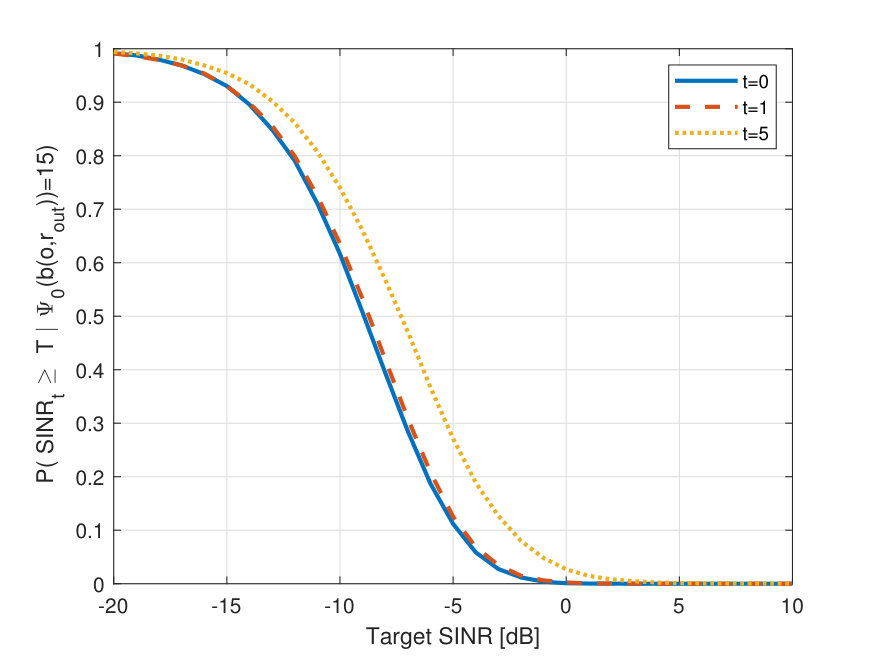 Figure 1
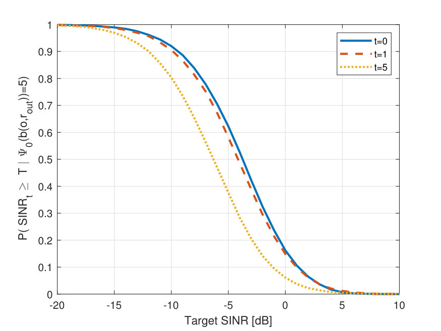 Figure 2
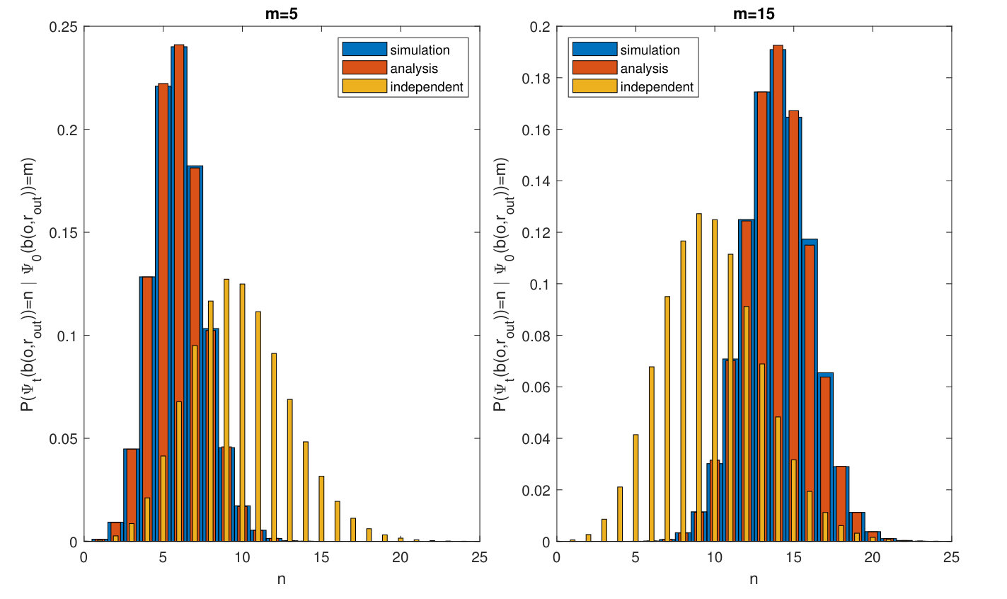 Figure 3
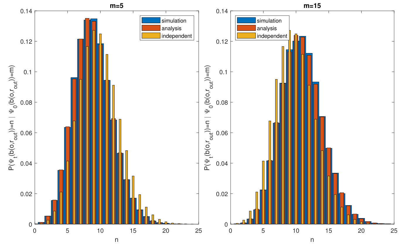 Figure 4
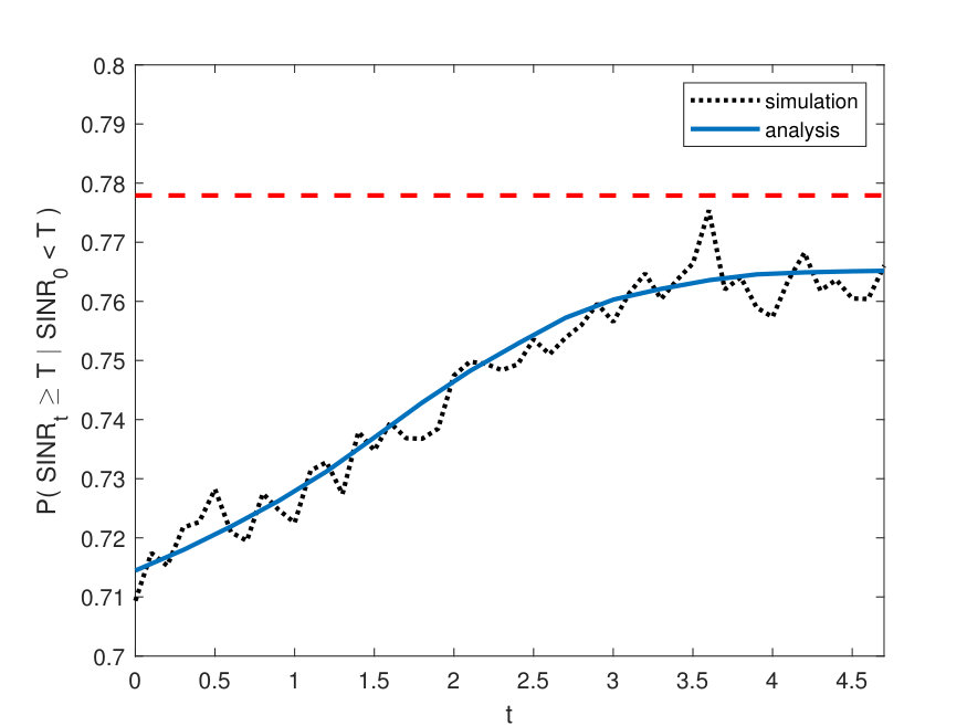 Figure 5
Peer Reviews
No public reviews on file for this paper yet. If you reviewed it on a platform where reviews are public (OpenReview, ICLR, NeurIPS, ICML), you can paste yours below so the community can read it here.
Videos
No videos yet. Explain this paper in a talk, walkthrough, or lecture? Add one.
On the Effect of Temporal Correlation on Joint Success Probability and Distribution of Number of Interferers in Mobile UAV Networks
Mohammad Salehi and Ekram Hossain The authors are with the Department of Electrical and Computer Engineering, University of Manitoba, Canada (Email: [email protected], [email protected]). This work was supported by a Discovery Grant from the Natural Sciences and Engineering Research Council of Canada (NSERC).
Abstract
Unmanned aerial vehicle (UAV)-aided terrestrial cellular networks is being considered as one of the disruptive technologies that can address the beyond 5G (B5G)/6G requirements. With mobile UAVs, since locations of the serving UAVs and the interfering UAVs can vary over time, interference and other performance metrics become temporally correlated. In this letter, we analyze the effect of temporal correlation on the joint success probability and the distribution of the number of interferers for mobile UAV networks. The analytical results will be useful, for example, to design error recovery protocols in these networks.
Index Terms:
Unmanned aerial vehicle (UAV), interference, success probability, stochastic geometry, Poisson point process, mobility, correlation.
I Introduction and Motivation
To meet the B5G and 6G requirements, UAVs can be employed to complement the terrestrial base stations to provide wireless communications service to the mobile users. Depending on the system model, different point processes from stochastic geometry have been used in the existing literature to model a UAV network and study downlink communication performance in different scenarios (e.g. in [1], [2, 3, 4], [5]). However, all of the existing work on static and mobile UAV scenarios only consider one time slot. Since locations of UAVs are spatially and temporally correlated, interference and other performance metrics that depend on the locations of the nodes are also spatially (at different locations in the network) and temporally (at different time slots) correlated [6]. Therefore, results that are derived for one time slot cannot be easily extended to study the network performance over time.
In this letter, we study the effect of correlation on the joint success probability (i.e. the joint probability of success at two time instants) and the distribution of the number of interferers in a mobile UAV network. The motivation for this study is as follows: (i) At a typical receiver, success probability is the probability that the signal-to-interference-plus-noise ratio (SINR) is greater than a target threshold. Due to correlation, unsuccessful transmission at time [math] (reference time) implies that probability of successful retransmission at time tends to [math] as , i.e. probability of successful retransmission at time is not independent of the success probability at time 0. Therefore, the joint transmission probability can be exploited to design error recovery (e.g. ARQ [Automatic Repeat reQuest]) strategies. (ii) Given that co-channel UAVs cause interference at the typical user at time [math], the number of interferers at time depends on , the initial locations of all UAVs, mobility parameters (velocity and direction) of all UAVs, and UAVs’ antenna patterns. With the distribution of the number of interferers at time given the number of interferers at time [math] is , we can study the success probability-latency tradeoff. For example, in some scenarios (depending on the network parameters), postponing a transmission for time can increase the success probability. Note that we only consider the effect correlation at the typical user at two different time instants (i.e. temporal correlation).
The rest of the letter is organized as follows. Section II states the system model and assumptions. The analytical results on joint success probability and distribution of the number of interferers are presented in Section III. Section IV presents the numerical and simulation results and Section V concludes the letter.
II System Model and Assumptions
We assume all UAVs are positioned at the same height and projection of their initial locations onto plane follows a homogeneous Poisson point process (PPP) of intensity . Due to the stationarity of PPP, we can randomly select a typical UAV and consider its projected location as the origin of our coordination system . We assume each UAV is serving a user that is located beneath it at the ground level, i.e. UAVs are located such that the average received signal power at each user from its serving UAV is maximum. Thus, the typical user which is served by the typical UAV is located at the origin . Since is fixed, for the rest of the paper, when we discuss about UAVs’ locations we mean their projected locations onto the plane. Therefore, when we say a UAV is located at , it means the projected location of the UAV onto the plane is at and the UAV is at distance from the typical user, where denotes the 2-norm distance.
We assume that, after the first time slot, a fraction of UAVs (except the typical UAV) are mobile, i.e. denotes the probability that a UAV moves which is independent of its initial location and other UAVs’ locations. A mobile UAV that is initially located at , moves, for duration , with velocity in a random angle with respect to the direction to the typical UAV, where is uniformly distributed in the interval and is a random variable with probability density function (PDF) and cumulative distribution function (CDF) . We also denote UAV’s displacement due to mobility by ; therefore, The UAV’s projected location at time can be written as . We use to denote the projected locations of UAVs at time .
At time , channel between a UAV located at and the typical user at the origin is , where denotes the channel power coefficient and follows a gamma distribution with shape parameter and scale parameter (Nakagami fading) with the PDF is as follows:
[TABLE]
We assume that is independently and identically distributed across time and UAV location . also denotes the large-scale path loss, where is the path-loss exponent. We also denote the variance of thermal noise by .
UAV antenna downtilt angle is . We also use sectorized gain pattern to approximate UAV antenna gain. Specifically, we assume
[TABLE]
i.e. antenna gain is for all the angles within the main lobe of beam width and is for all the angles between and . Let us assume that a UAV is located at , and define and . When , where denotes a two dimensional ball with radius centred at , the UAV causes interference at the typical user with effective gain . When , the co-channel UAV causes interference at the typical user with effective gain , and when , there is no interference from the UAV to the typical user.
We study the effect of correlation between time instants [math] and on the joint success probability and the distribution of the number of interferers111Due to stationarity and ergodicity of our model, our results can be used for time instants and , where .. Based on our system model, the total received interference at the typical user at time 0 is
[TABLE]
where, according to Slivnyak’s theorem, is a PPP with intensity . denotes the indicator function. The total received interference at the typical user at time can be written as
[TABLE]
where is 1 when node is mobile, otherwise is zero; therefore, is a Bernoulli random variable with parameter . When , the projected location of the UAV onto plane, at time , is at distance from the origin. Thus, the SINRs at the typical user at time instants 0 and are, respectively, as follows:
[TABLE]
III Analytical Results
III-A Joint Success Probability
In the following theorem, we derive the joint success probability at time instants 0 and .
Theorem 1**.**
Joint Success probability at time instants 0 and can be obtained by
[TABLE]
where
[TABLE]
Proof:
[TABLE]
where (a) is obtained by averaging over and . The expectation in (b) can also be obtained by averaging with respect to , , , fading power gains, and applying PGFL of PPP. ∎
Similar to Theorem 1, we can derive the transmission success probability at time 0 (or ).
[TABLE]
where the expectations in (LABEL:eq:success_at_0) and (LABEL:eq:success_at_t) can be obtained by substituting and in (1), respectively. To study the effect of correlation in mobile UAV networks, in the following, we derive the probability that the typical UAV has a successful transmission at time , given that the transmission at 0 is unsuccessful, i.e.
[TABLE]
Using Fortuin-Kasteleyn-Ginibre (FKG) inequality, one can show that .
III-B Distribution of the Number of Interferers
First we calculate , i.e. the probability that the projected location of a mobile UAV at time is in given its initial projected location is at . This probability, which is provided in the following lemma will be used to derive the distribution of the number of interferers.
Lemma 1**.**
The probability that the projected location of a mobile UAV at time is in given its initial projected location is at , denoted by , can be derived as
[TABLE]
Proof:
[TABLE]
∎
A UAV can cause interference at the typical user if its projected location is within . Therefore, at time 0, the number of interferers is a Poisson random variable with mean . In the following, we derive the distribution of the number of interferers at time given that initially the number of interferers is .
Theorem 2**.**
The probability that there are interferers at time given that initially the number of interferers is is
[TABLE]
where .
Proof:
Theorem 2 can be obtained by using
[TABLE]
Given , we can consider as a superposition of two independent point processes: i) a uniform BPP with number of points in , and ii) a PPP with intensity function . Therefore, we have
[TABLE]
where (a) is obtained by using probability generating functional (PGFL) of PPP. Finally, Theorem 2 is obtained by substituting (5) in (4), and employing the general Leibniz rule for the -th derivative of a product of two functions. ∎
We can also show that mean number of arrival of interferers (mean number of UAVs that only cause interference at the typical user at time ) is equal to
[TABLE]
and mean number of departure of interferers (mean number of UAVs that only cause interference at the typical user at time [math]) is
[TABLE]
As derived in Theorem 2, due to mobility of UAVs, the number of interferers is different in different time slots, and depending on the network parameters the mean number of interferers may increase or decrease. When the mean number of interferers increases, i.e. the mean number of arrivals is greater than mean number of departures, retransmitting an unsuccessfully received packet may not be helpful, while when the mean number of interferers decreases, if there is no stringent latency constraint, the typical UAV should postpone the transmission to increase reliability.
IV Numerical and Simulation Results
Distribution of the number of interferers at and , given, at time 0, the number of interferers is is illustrated in Fig. 1(a) and (b), respectively, for and . When , at (), mean number of arrivals is about 2 (8) and mean number of departures is about 1 (4). Thus, retransmitting an unsuccessfully received packet may not be helpful in this scenario. On the other hand, for , at (), the mean number of arrivals and departures are about 2 (8) and 3 (12), respectively. Therefore, when there is no strict latency constraint, postponing the transmission for time provides a higher reliability. Moreover, to study the effect of correlation on the distribution of the number of interferers, in Fig. 1, we compare the results with the independent scenario, where the distribution of the number of interferers follows a Poisson random variable with mean . As can be seen, the correlation decreases as the time gap increases.
Fig. 2 illustrates the variation in conditional success probability at time with different target SINR, given that, at time 0, the number of interferers is . These results are obtained from simulations. For , the conditional success probability decreases as increases, while for the conditional success probability increases as increases.
We also study the effect of temporal correlation in mobile UAV networks in Fig. 3. Specifically, we have illustrated the success probability at time given initial transmission attempt at time [math] fails. As the time gap between the two transmission attempts, denoted by , increases, success probability increases since the correlation between the two time instants decreases. We also compare our results with the independent scenario (shown by the red dashed line). As is evident, as increases we can ignore the correlation.
V Conclusion
We have studied the effect of temporal correlation on the distribution of the number of interferers and success probability in mobile UAV networks. We have shown that in some scenarios, this correlation can be exploited by postponing a transmission in order to increase the success probability (or reliability). As the time gap between two transmission attempts increases the effect of correlation decreases. Our results can be used to optimize the error recovery protocols (e.g. ARQ protocols) and study the rate-reliability-latency tradeoffs in UAV networks. In this letter, we have only considered the effect of temporal correlation on the downlink performance of a user served by a static UAV in a network that includes both static and mobile UAVs. For future work, we can similarly study the effect of temporal correlation on the performance of a user served by mobile UAVs in the same network.
The reference list from the paper itself. Each links out to its DOI / PubMed record.
- 1[1] E. Turgut and M. C. Gursoy, “Downlink analysis in unmanned aerial vehicle (uav) assisted cellular networks with clustered users,” IEEE Access , vol. 6, pp. 36 313–36 324, 2018.
- 2[2] B. Galkin, J. Kibilda, and L. A. Da Silva, “A stochastic geometry model of backhaul and user coverage in urban uav networks,” Co RR , vol. abs/1710.03701, 2017.
- 3[3] M. M. Azari, F. Rosas, A. Chiumento, and S. Pollin, “Coexistence of terrestrial and aerial users in cellular networks,” in 2017 IEEE Globecom Workshops (GC Wkshps) , Dec 2017, pp. 1–6.
- 4[4] D. Kim, J. Lee, and T. Q. S. Quek, “Performance analysis for multi-layer unmanned aerial vehicle networks,” in 2018 IEEE Globecom Workshops (GC Wkshps) , Dec 2018, pp. 1–6.
- 5[5] P. K. Sharma and D. I. Kim, “Random 3d mobile uav networks: Mobility modeling and coverage probability,” IEEE Transactions on Wireless Communications , 2019.
- 6[6] R. K. Ganti and M. Haenggi, “Spatial and temporal correlation of the interference in aloha ad hoc networks,” IEEE Communications Letters , vol. 13, no. 9, pp. 631–633, 2009.