Geometric renormalization unravels self-similarity of the multiscale human connectome
Muhua Zheng, Antoine Allard, Patric Hagmann, Yasser Alem\'an-G\'omez,, M. \'Angeles Serrano

TL;DR
This study reveals that the human brain's structural connectivity exhibits self-similarity across multiple scales, and a geometric renormalization model effectively predicts these multiscale properties, suggesting simple underlying organizing principles.
Contribution
The paper introduces a geometric renormalization approach that uncovers self-similarity in multiscale human connectomes, advancing understanding of brain architecture across resolutions.
Findings
Brain connectomes are self-similar across multiple resolutions.
A geometric network model predicts multiscale connectome properties.
Simple organizing principles underlie the brain's multiscale structure.
Abstract
Structural connectivity in the brain is typically studied by reducing its observation to a single spatial resolution. However, the brain possesses a rich architecture organized over multiple scales linked to one another. We explored the multiscale organization of human connectomes using datasets of healthy subjects reconstructed at five different resolutions. We found that the structure of the human brain remains self-similar when the resolution of observation is progressively decreased by hierarchical coarse-graining of the anatomical regions. Strikingly, a geometric network model, where distances are not Euclidean, predicts the multiscale properties of connectomes, including self-similarity. The model relies on the application of a geometric renormalization protocol which decreases the resolution by coarse-graining and averaging over short similarity distances. Our results suggest…
Click any figure to enlarge with its caption.
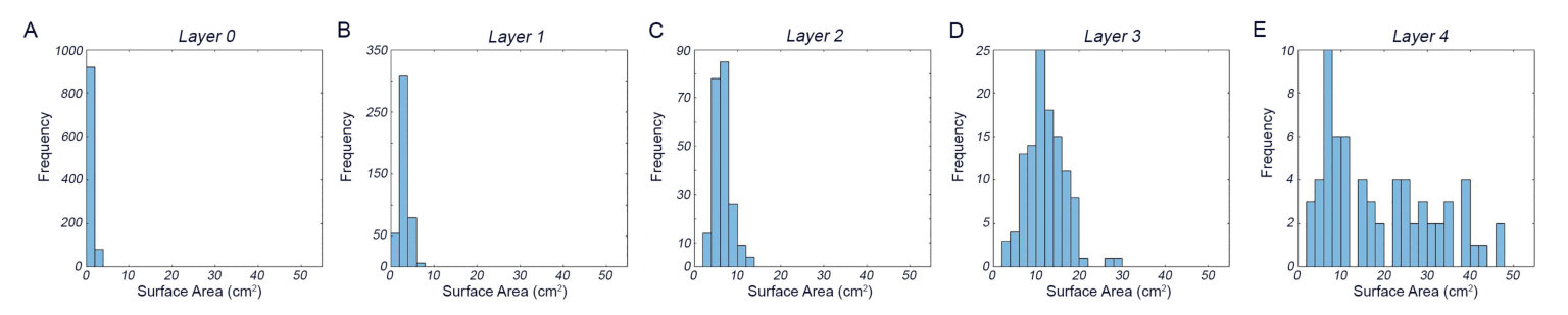 Figure 1
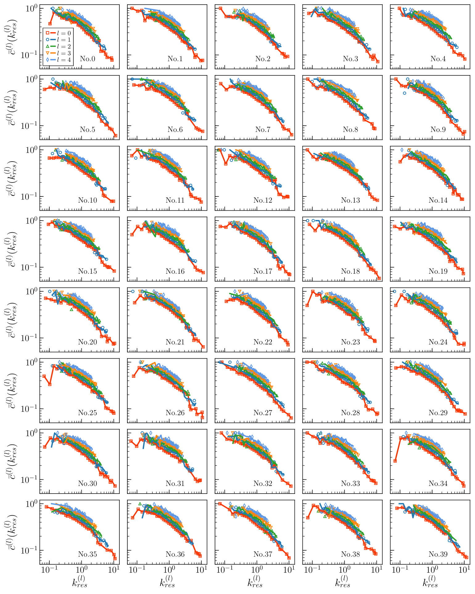 Figure 2
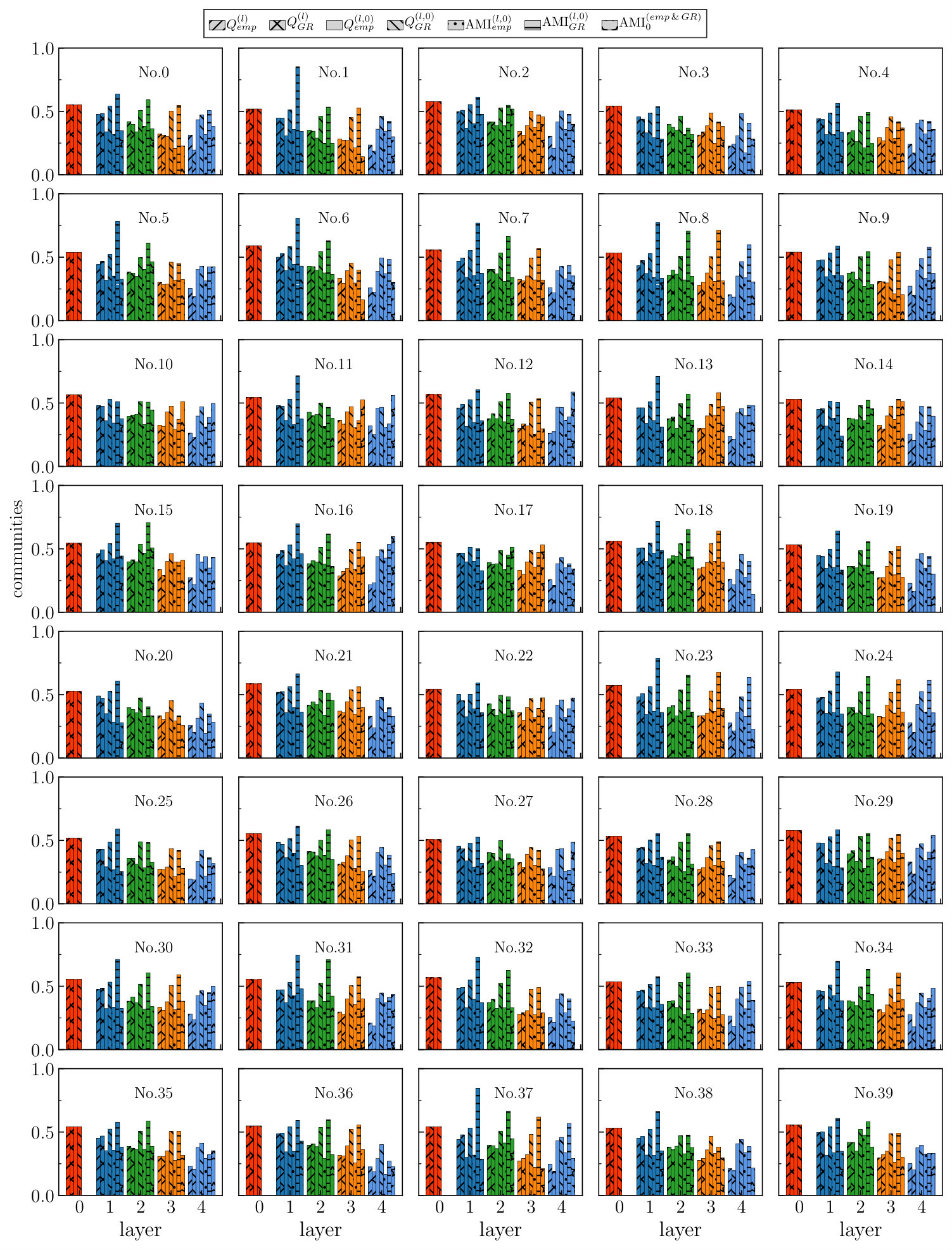 Figure 3
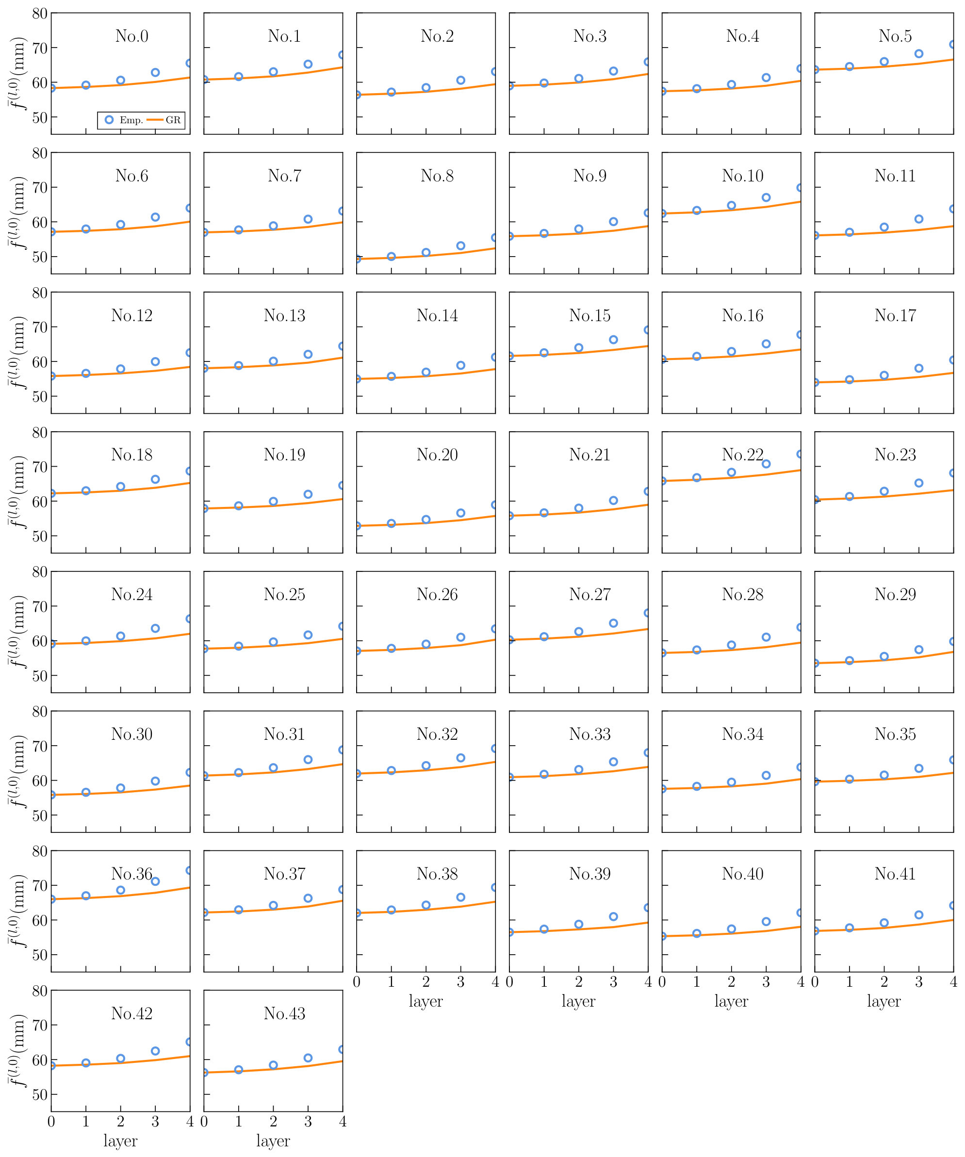 Figure 4
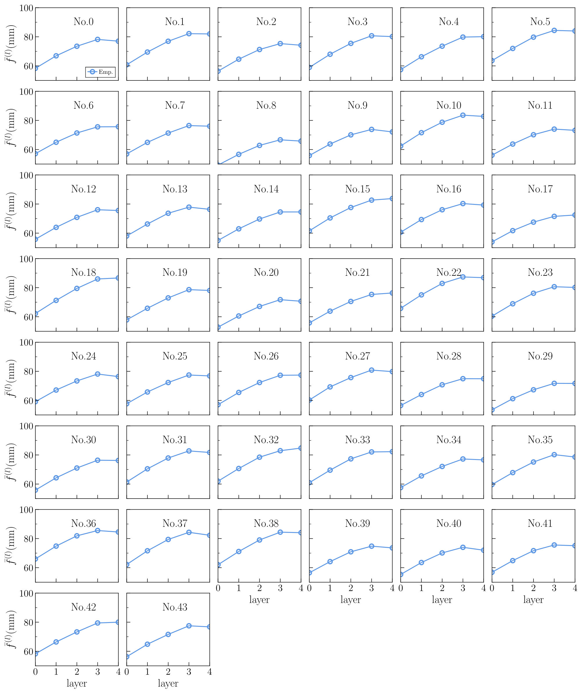 Figure 5
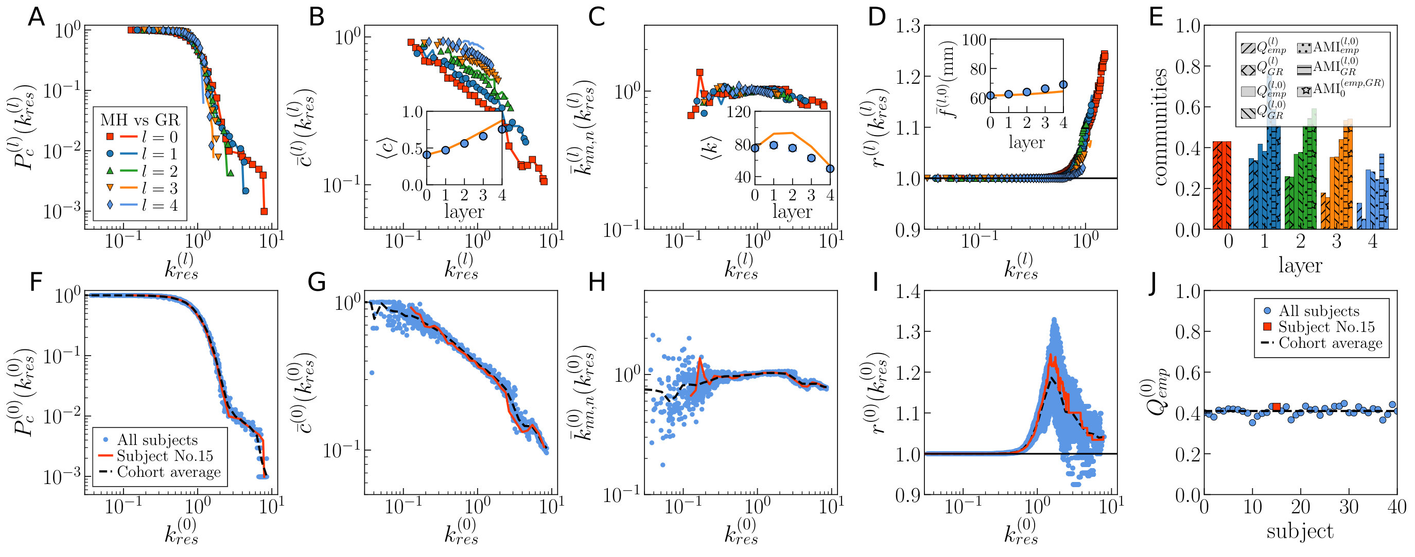 Figure 1
 Figure 2
 Figure 3
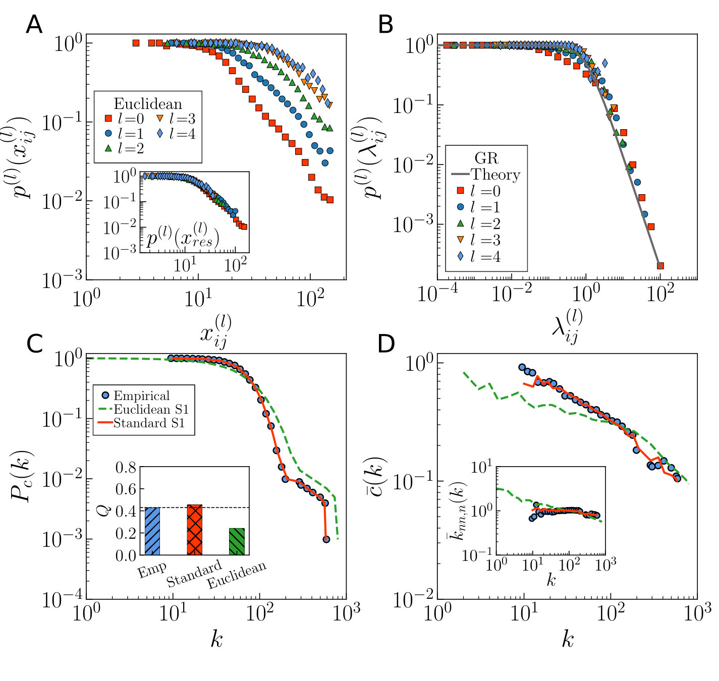 Figure 4
 Figure 5
 Figure 11
 Figure 12
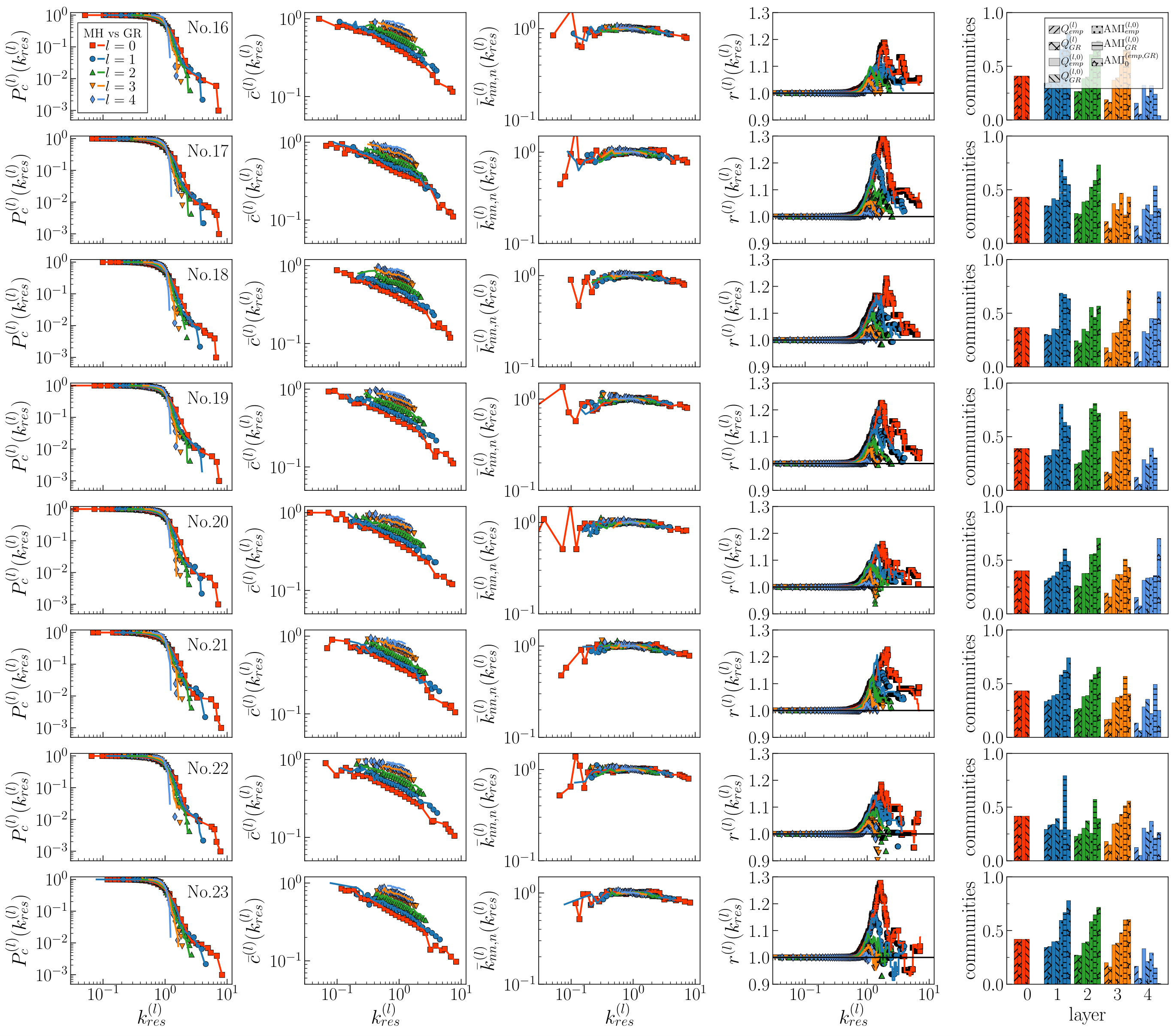 Figure 13
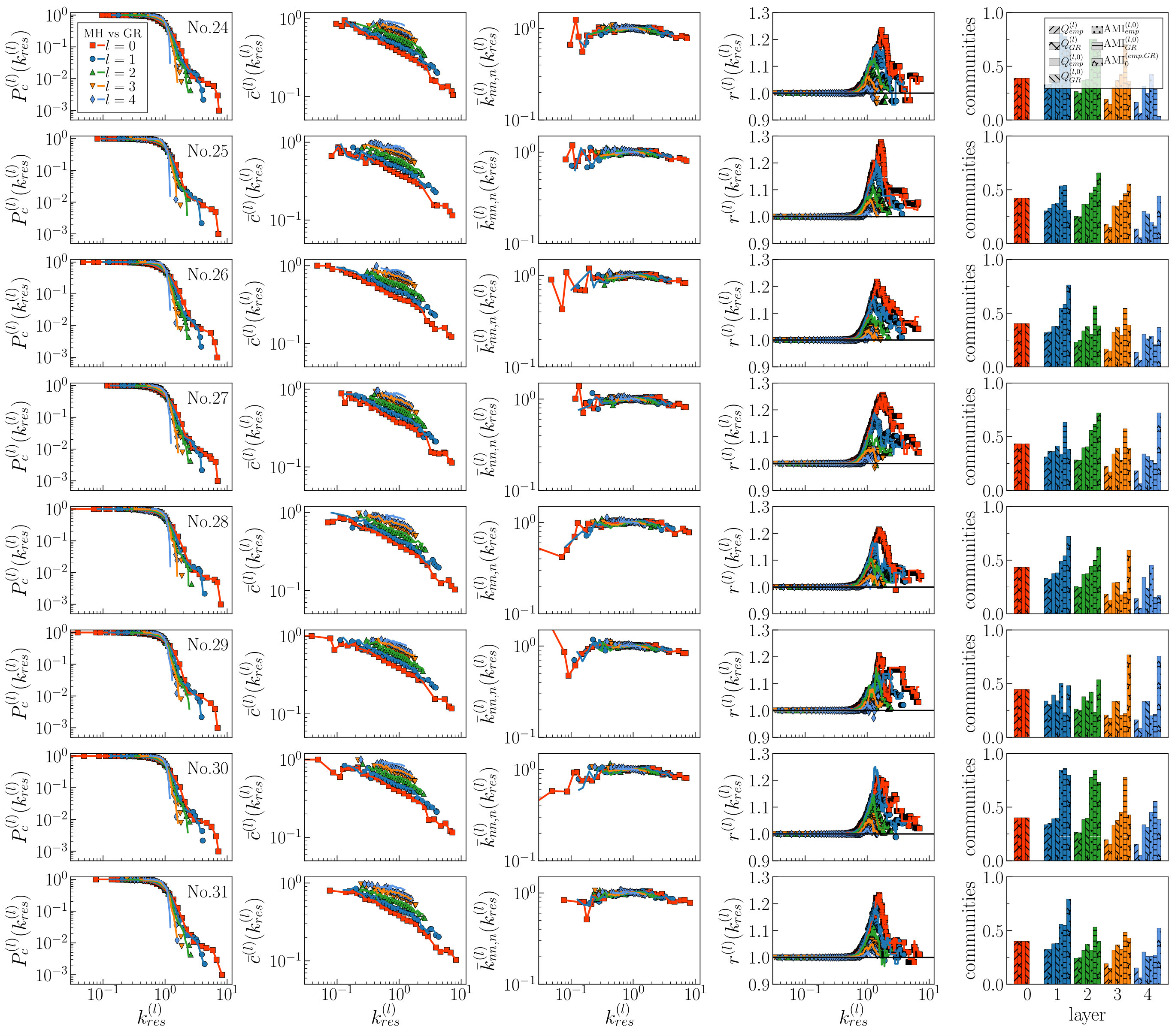 Figure 14
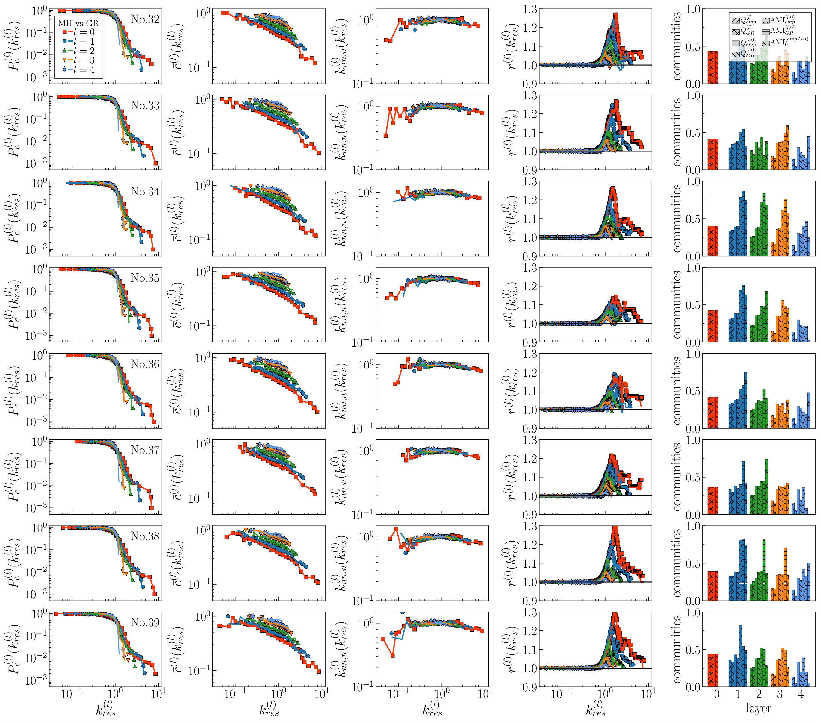 Figure 15
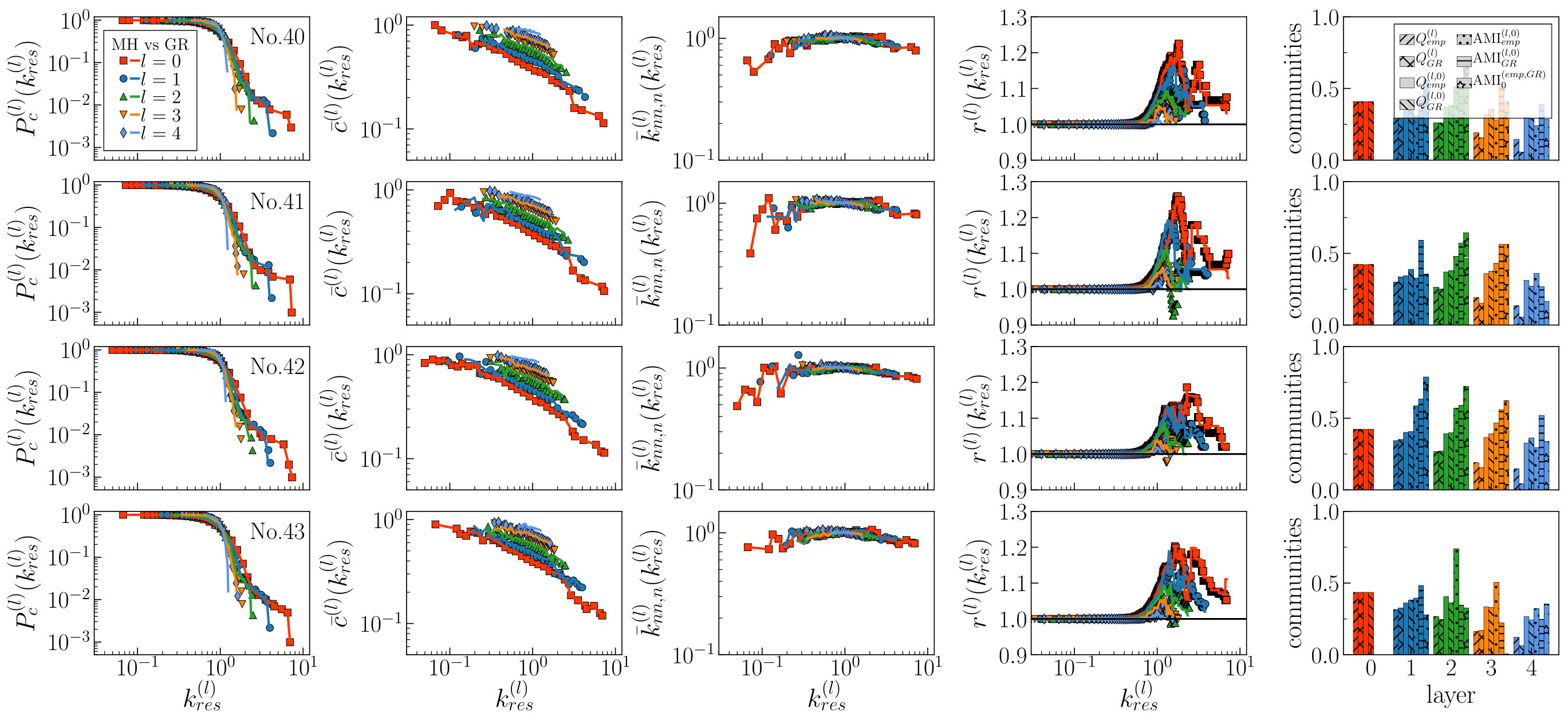 Figure 16
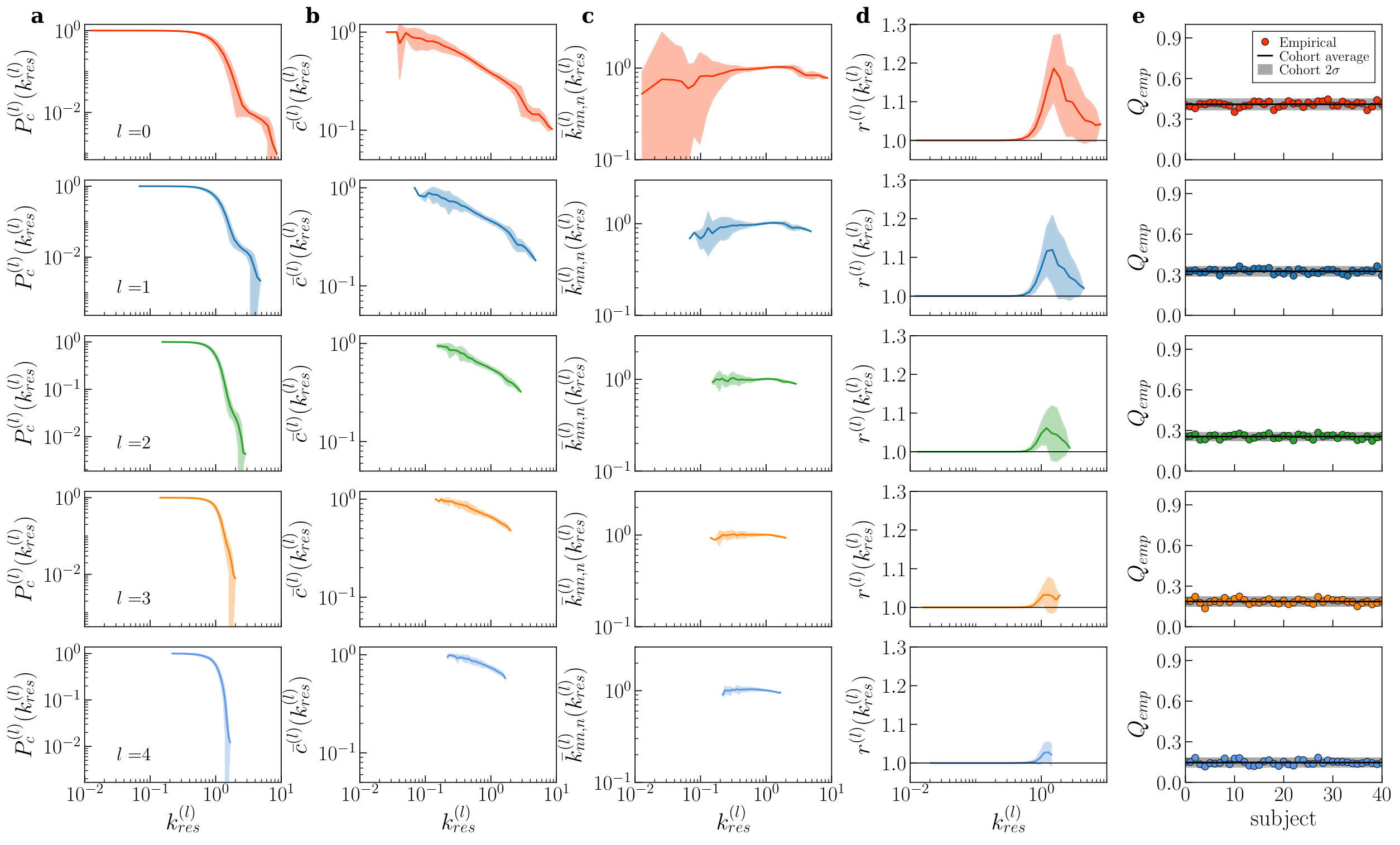 Figure 17
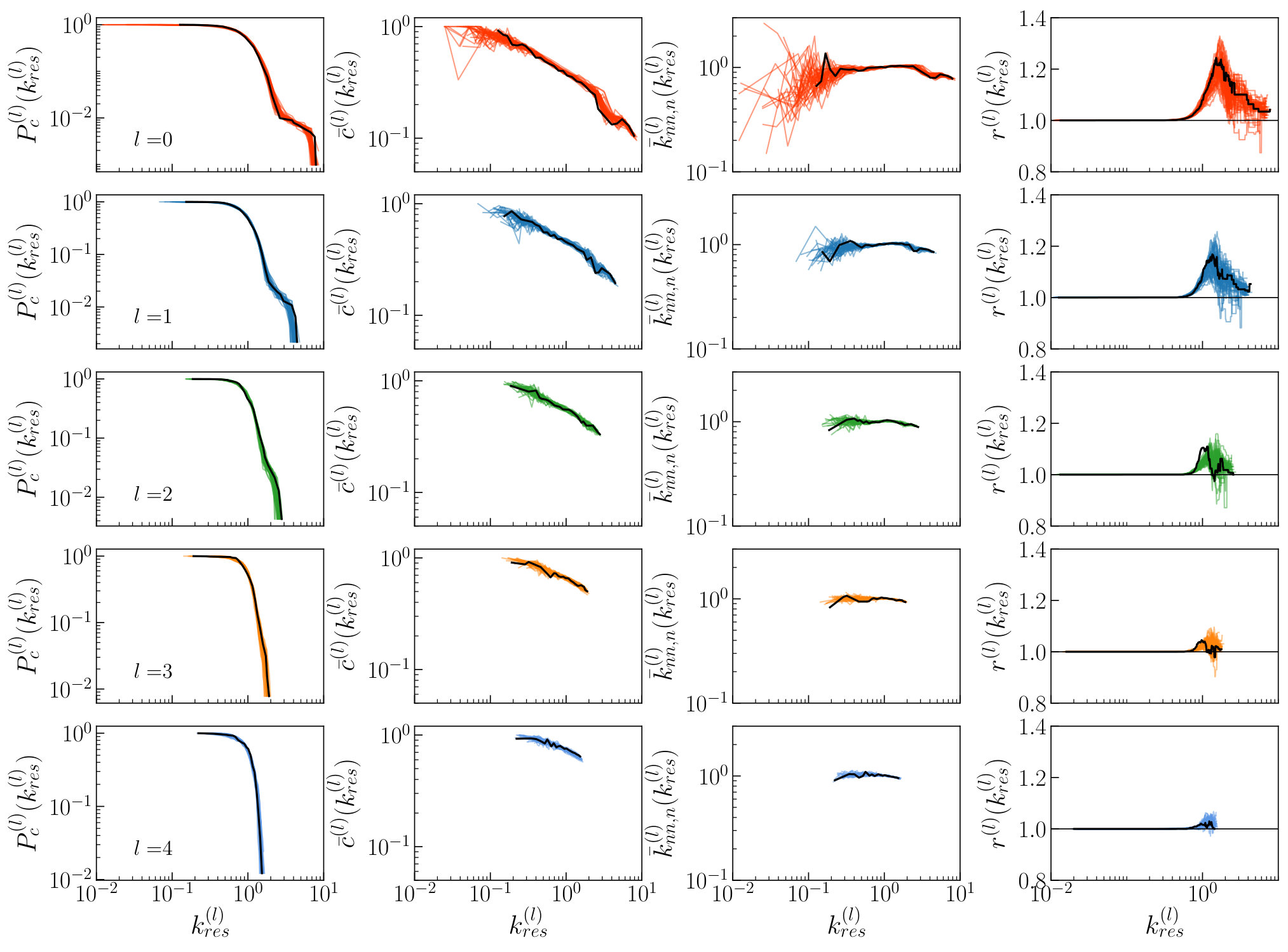 Figure 18
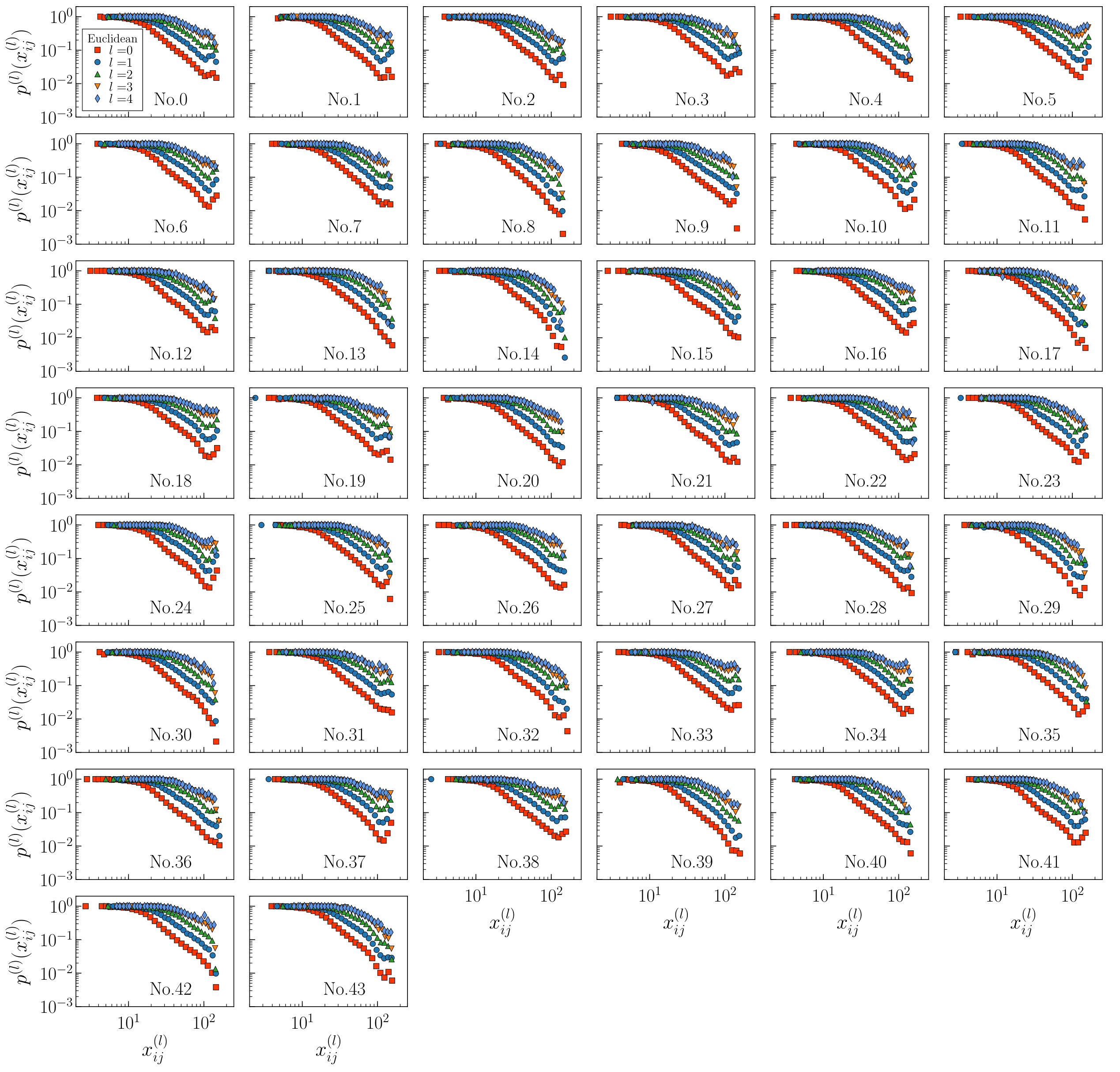 Figure 19
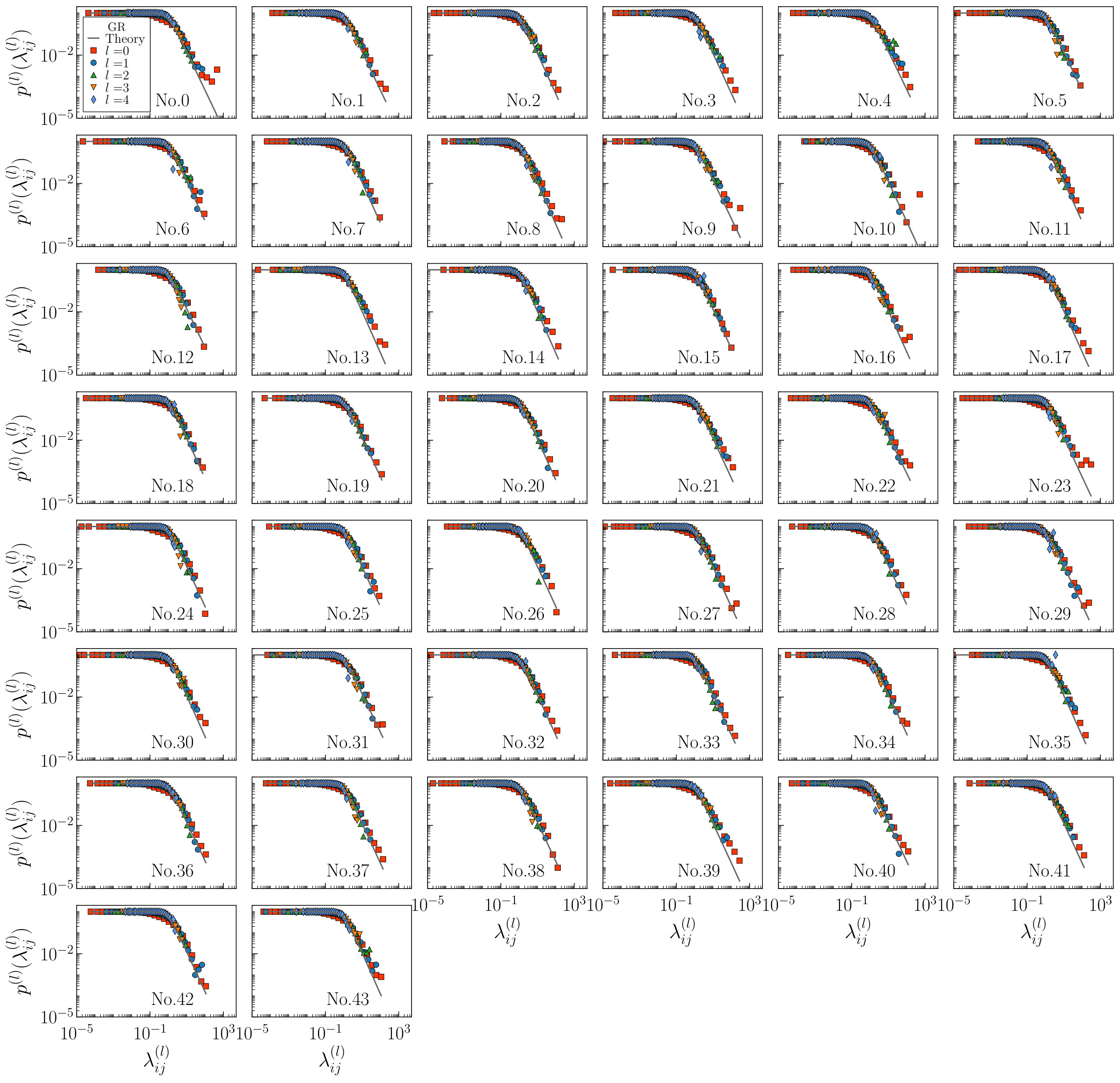 Figure 20
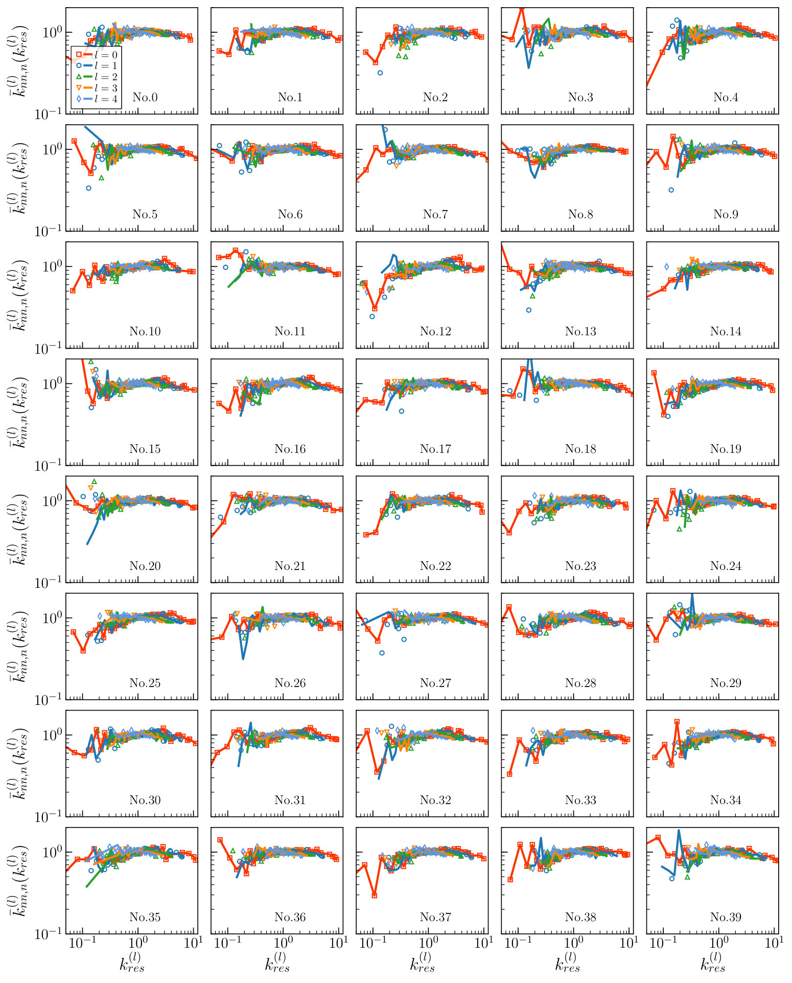 Figure 21
 Figure 22
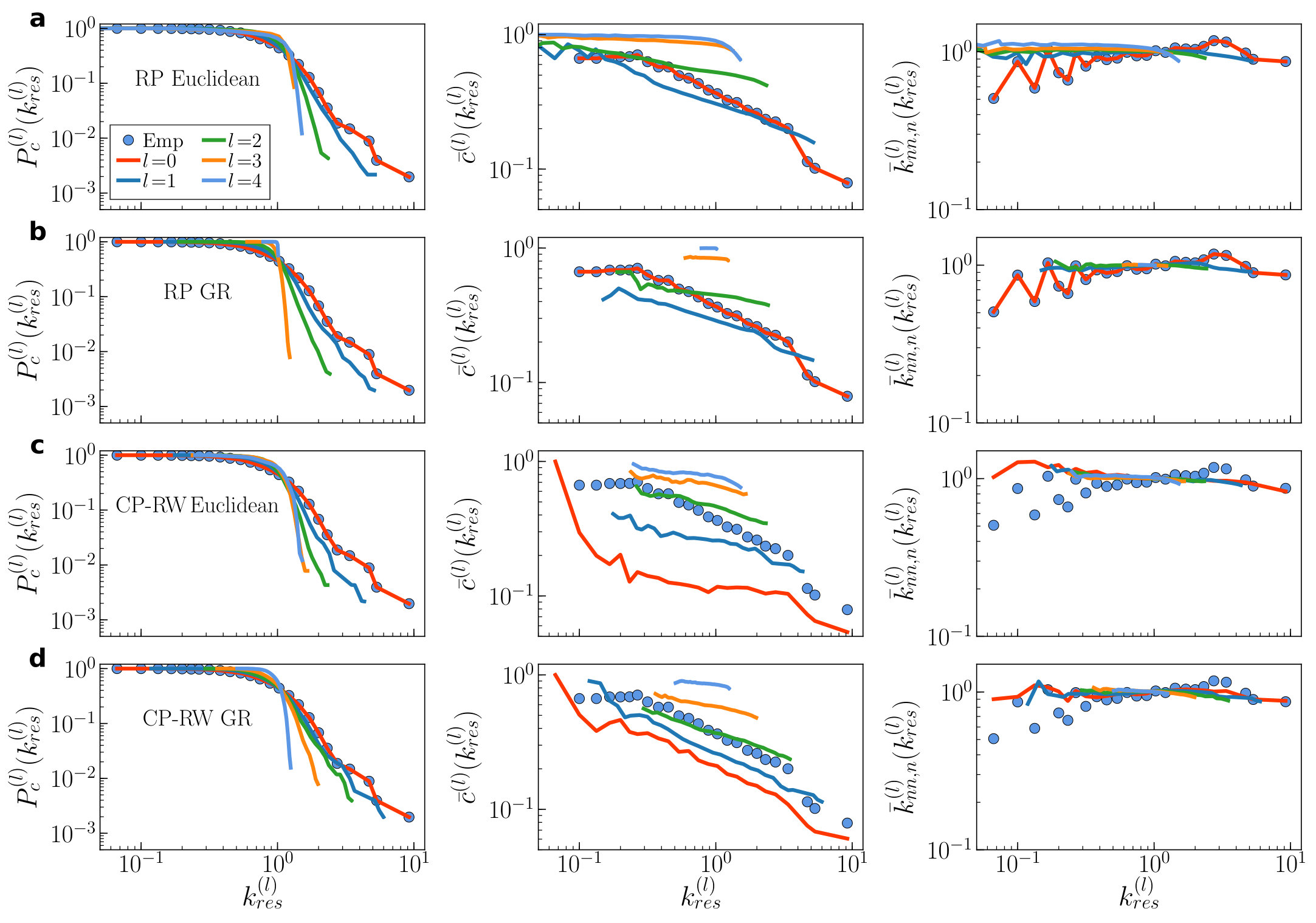 Figure 23
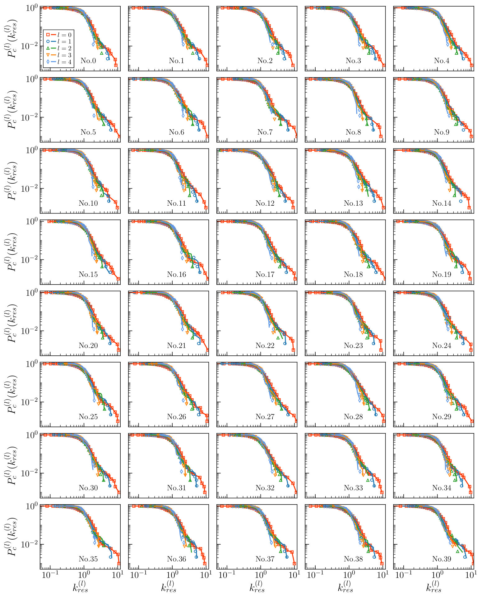 Figure 24
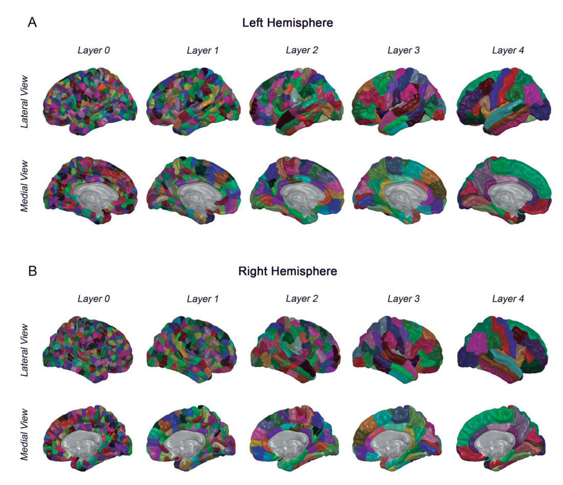 Figure 25
 Figure 26
 Figure 27
 Figure 28
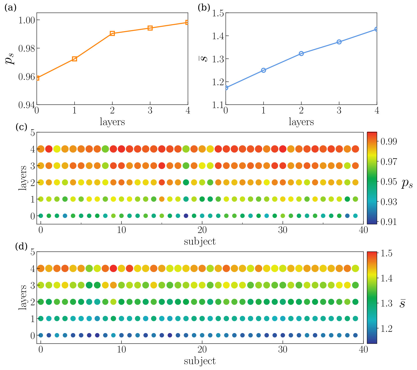 Figure 6
 Figure 30
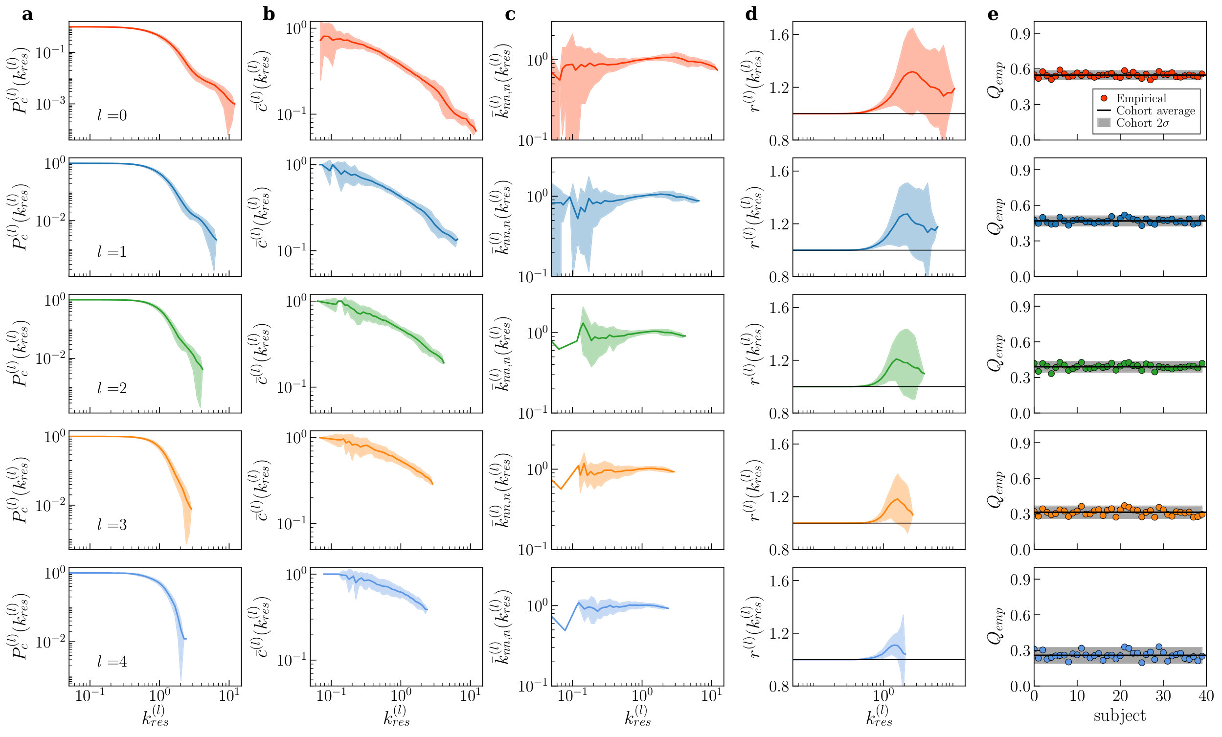 Figure 31
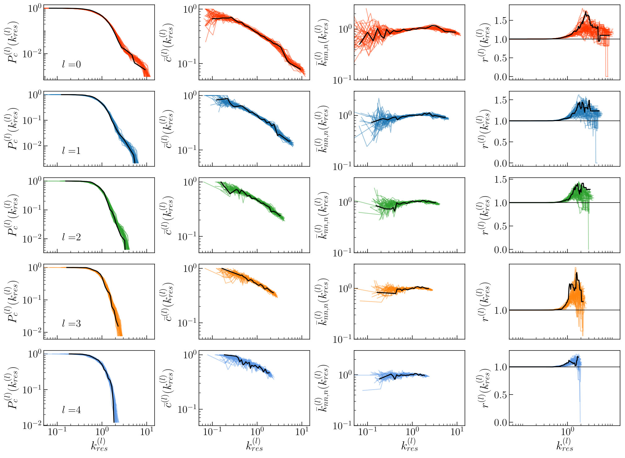 Figure 32
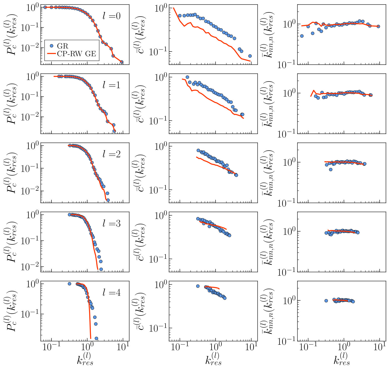 Figure 33
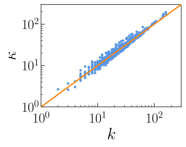 Figure 34
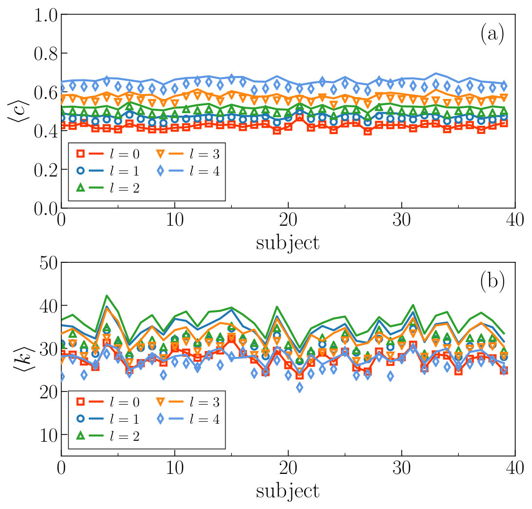 Figure 35
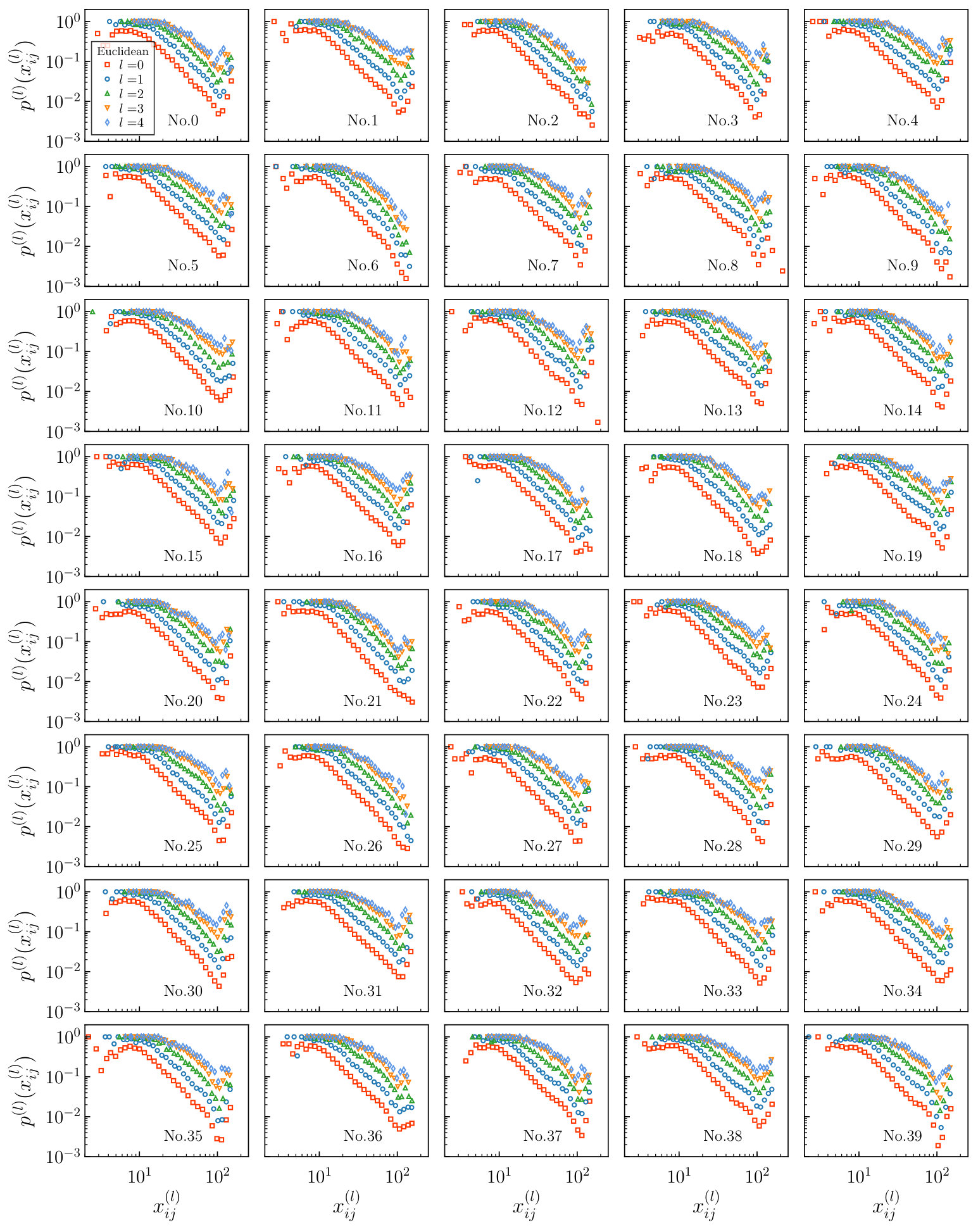 Figure 36
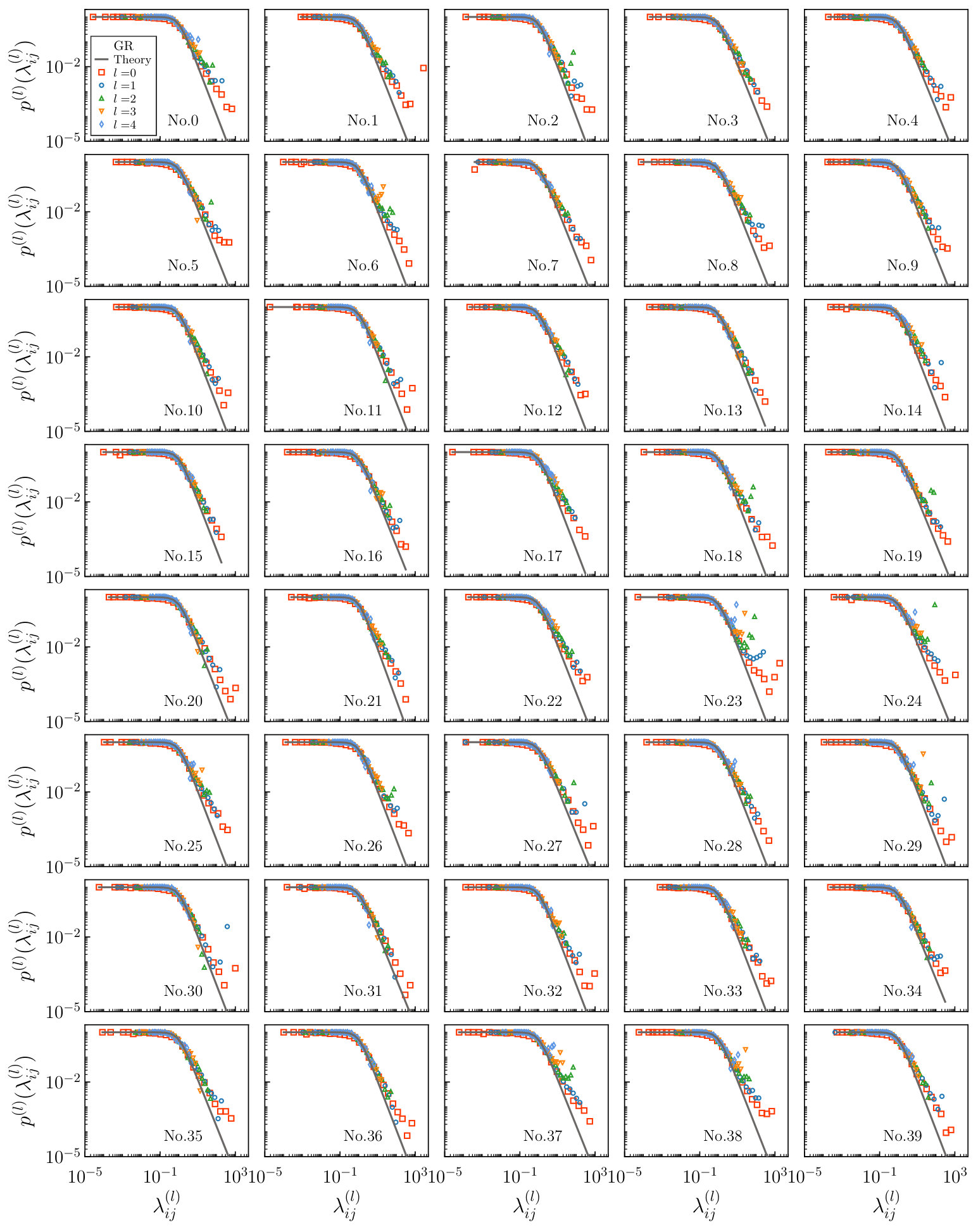 Figure 37
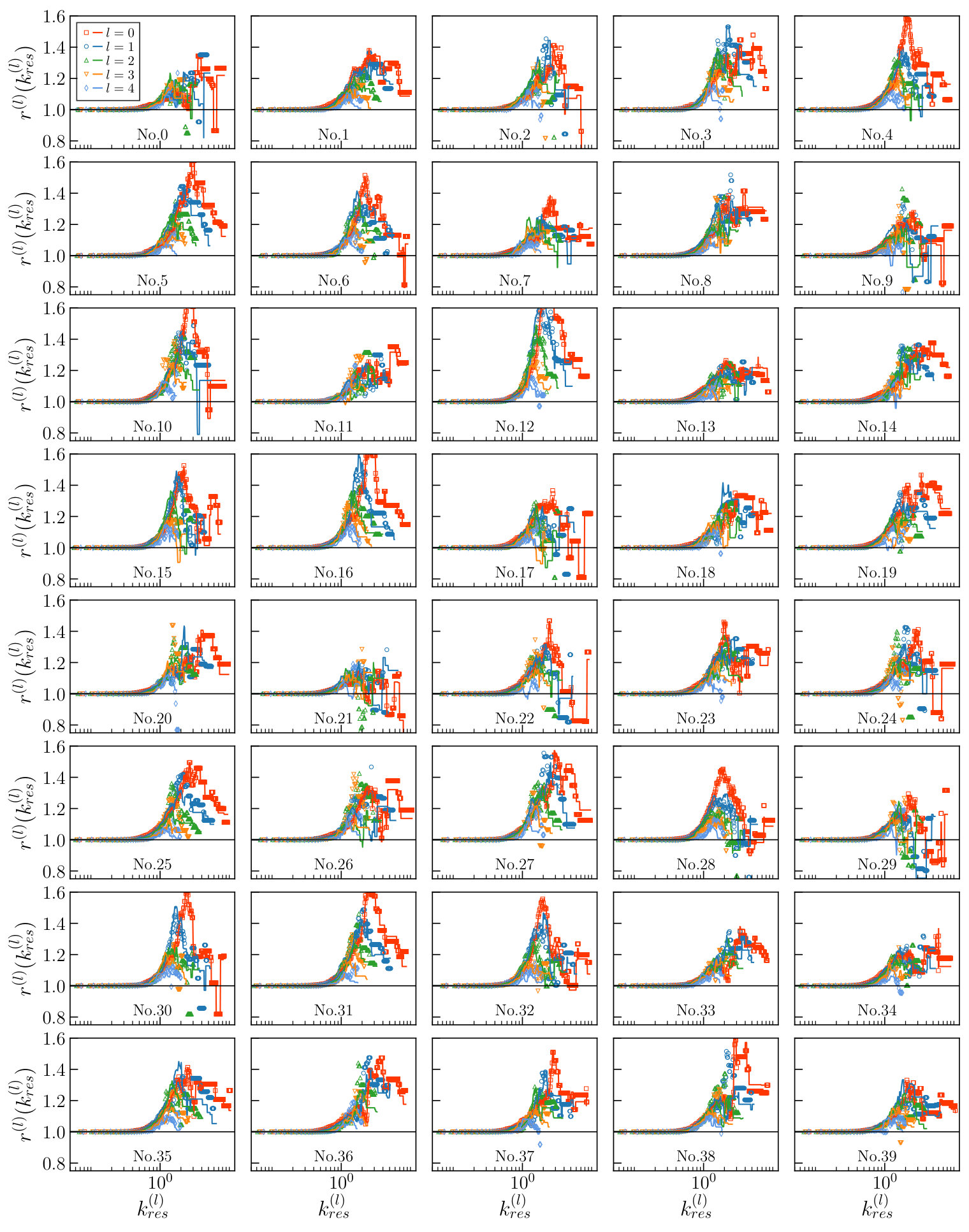 Figure 38
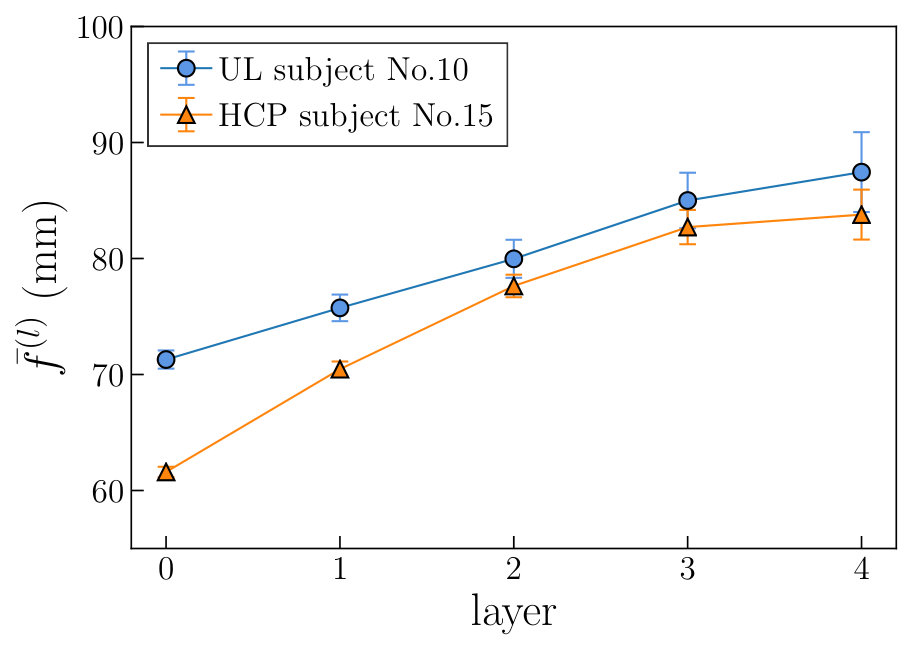 Figure 1
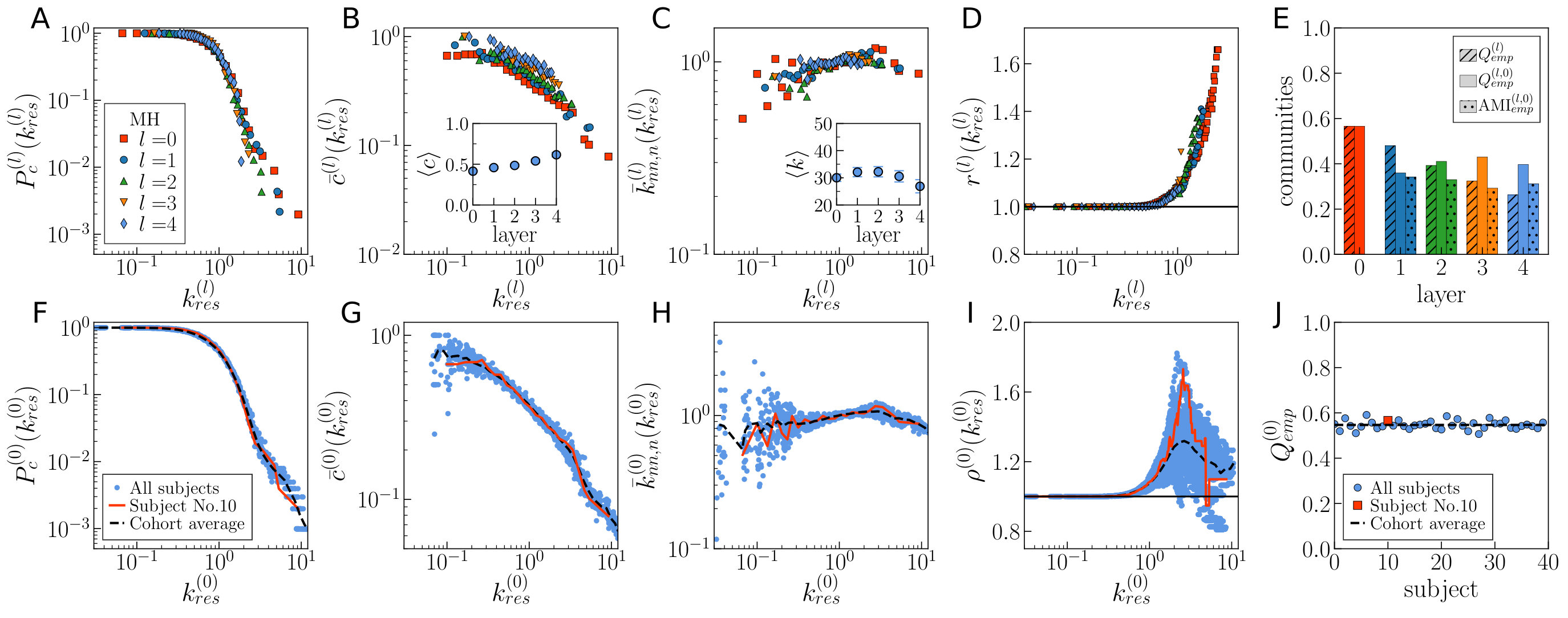 Figure 2
| Subject | Layer | |||||||||||
|---|---|---|---|---|---|---|---|---|---|---|---|---|
| No. 0 | 0 | 1009 | 14470 | 0.03 | 28.680.669 | 0.430.005 | 65.8243.675 | -0.016 | 0.55 | 5 | 1.96 | 0.011 |
| 1 | 461 | 7177 | 0.07 | 31.140.825 | 0.470.006 | 68.8244.082 | 0.005 | 0.48 | 5 | 2.22 | 0.011 | |
| 2 | 233 | 3586 | 0.13 | 30.780.937 | 0.500.008 | 72.7445.021 | 0.031 | 0.42 | 5 | 2.41 | 0.012 | |
| 3 | 128 | 1744 | 0.21 | 27.251.031 | 0.560.012 | 74.8046.285 | 0.040 | 0.32 | 3 | 2.63 | 0.014 | |
| 4 | 82 | 962 | 0.29 | 23.461.102 | 0.620.016 | 74.3947.996 | 0.021 | 0.31 | 3 | 3.08 | 0.018 | |
| No. 1 | 0 | 1010 | 14406 | 0.03 | 28.530.729 | 0.420.005 | 66.3844.958 | -0.003 | 0.52 | 5 | 1.93 | 0.011 |
| 1 | 461 | 7195 | 0.07 | 31.210.944 | 0.460.006 | 70.4645.278 | 0.003 | 0.45 | 6 | 2.11 | 0.011 | |
| 2 | 233 | 3893 | 0.14 | 33.421.158 | 0.500.008 | 76.4446.113 | -0.012 | 0.35 | 3 | 2.26 | 0.011 | |
| 3 | 128 | 1992 | 0.25 | 31.121.257 | 0.570.010 | 80.3347.629 | -0.039 | 0.28 | 3 | 2.48 | 0.012 | |
| 4 | 82 | 1129 | 0.34 | 27.541.328 | 0.630.013 | 83.1150.287 | -0.080 | 0.23 | 4 | 2.78 | 0.015 | |
| No. 2 | 0 | 1014 | 13671 | 0.03 | 26.960.638 | 0.440.005 | 62.4542.759 | 0.008 | 0.58 | 6 | 2.00 | 0.012 |
| 1 | 462 | 6833 | 0.06 | 29.580.812 | 0.460.006 | 67.3243.889 | 0.027 | 0.50 | 5 | 2.19 | 0.012 | |
| 2 | 233 | 3599 | 0.13 | 30.890.954 | 0.490.008 | 73.0145.070 | 0.056 | 0.42 | 4 | 2.41 | 0.012 | |
| 3 | 128 | 1806 | 0.22 | 28.221.031 | 0.550.011 | 74.9545.415 | 0.043 | 0.34 | 4 | 2.63 | 0.014 | |
| 4 | 82 | 978 | 0.29 | 23.851.131 | 0.630.015 | 75.1247.046 | -0.035 | 0.30 | 3 | 3.23 | 0.018 | |
| No. 3 | 0 | 1011 | 12991 | 0.03 | 25.700.648 | 0.410.005 | 61.5143.188 | 0.003 | 0.54 | 7 | 1.89 | 0.012 |
| 1 | 462 | 6642 | 0.06 | 28.750.842 | 0.450.006 | 64.3243.813 | 0.029 | 0.46 | 4 | 2.08 | 0.011 | |
| 2 | 233 | 3581 | 0.13 | 30.741.016 | 0.490.008 | 69.0745.923 | 0.046 | 0.40 | 5 | 2.26 | 0.012 | |
| 3 | 128 | 1888 | 0.23 | 29.501.135 | 0.550.011 | 74.3849.242 | 0.049 | 0.31 | 3 | 2.48 | 0.013 | |
| 4 | 82 | 1074 | 0.32 | 26.201.302 | 0.630.015 | 79.4953.949 | 0.005 | 0.23 | 2 | 2.78 | 0.015 | |
| No. 4 | 0 | 1014 | 15879 | 0.03 | 31.320.778 | 0.410.005 | 72.3250.544 | 0.014 | 0.51 | 6 | 1.85 | 0.009 |
| 1 | 462 | 7896 | 0.07 | 34.180.999 | 0.460.006 | 76.9852.410 | 0.036 | 0.44 | 4 | 2.08 | 0.010 | |
| 2 | 233 | 4069 | 0.15 | 34.931.165 | 0.500.008 | 81.5653.710 | 0.057 | 0.33 | 4 | 2.26 | 0.010 | |
| 3 | 128 | 2077 | 0.26 | 32.451.254 | 0.570.010 | 83.7954.812 | 0.042 | 0.29 | 3 | 2.63 | 0.012 | |
| 4 | 82 | 1177 | 0.35 | 28.711.408 | 0.660.013 | 86.8558.033 | -0.027 | 0.24 | 3 | 2.93 | 0.014 | |
| No. 5 | 0 | 1014 | 14340 | 0.03 | 28.280.698 | 0.410.005 | 65.3042.579 | -0.013 | 0.54 | 5 | 1.89 | 0.011 |
| 1 | 462 | 7175 | 0.07 | 31.060.900 | 0.450.006 | 69.2343.346 | -0.003 | 0.44 | 5 | 2.11 | 0.011 | |
| 2 | 233 | 3719 | 0.14 | 31.921.043 | 0.480.007 | 73.6443.925 | 0.008 | 0.38 | 4 | 2.22 | 0.011 | |
| 3 | 128 | 1919 | 0.24 | 29.981.141 | 0.550.009 | 76.8545.317 | 0.004 | 0.30 | 4 | 2.48 | 0.013 | |
| 4 | 82 | 1137 | 0.34 | 27.731.260 | 0.630.012 | 79.3647.597 | -0.021 | 0.25 | 3 | 2.78 | 0.014 | |
| No. 6 | 0 | 1013 | 12660 | 0.02 | 25.000.653 | 0.440.005 | 57.0138.389 | -0.012 | 0.59 | 6 | 1.96 | 0.013 |
| 1 | 462 | 6519 | 0.06 | 28.220.865 | 0.480.007 | 61.1639.025 | -0.006 | 0.50 | 5 | 2.26 | 0.013 | |
| 2 | 233 | 3375 | 0.12 | 28.971.009 | 0.530.009 | 64.8739.810 | -0.014 | 0.43 | 4 | 2.52 | 0.013 | |
| 3 | 128 | 1712 | 0.21 | 26.751.080 | 0.570.012 | 68.3141.896 | -0.014 | 0.33 | 3 | 2.78 | 0.015 | |
| 4 | 82 | 1000 | 0.30 | 24.391.196 | 0.620.015 | 71.2745.710 | -0.017 | 0.26 | 4 | 3.00 | 0.017 | |
| No. 7 | 0 | 1014 | 13474 | 0.03 | 26.580.702 | 0.420.005 | 64.4543.876 | -0.023 | 0.56 | 6 | 1.89 | 0.011 |
| 1 | 462 | 6955 | 0.07 | 30.110.902 | 0.460.006 | 68.6945.530 | -0.012 | 0.47 | 4 | 2.11 | 0.011 | |
| 2 | 233 | 3651 | 0.14 | 31.341.019 | 0.500.007 | 73.5547.353 | -0.006 | 0.40 | 3 | 2.41 | 0.012 | |
| 3 | 128 | 1934 | 0.24 | 30.221.079 | 0.560.010 | 78.7250.132 | 0.000 | 0.32 | 4 | 2.63 | 0.013 | |
| 4 | 82 | 1076 | 0.32 | 26.241.201 | 0.620.014 | 81.3853.156 | -0.041 | 0.26 | 3 | 2.86 | 0.015 |
| Subject | Layer | |||||||||||
|---|---|---|---|---|---|---|---|---|---|---|---|---|
| No. 8 | 0 | 1002 | 13910 | 0.03 | 27.760.652 | 0.410.005 | 67.6545.004 | 0.017 | 0.53 | 5 | 1.89 | 0.011 |
| 1 | 462 | 7041 | 0.07 | 30.480.845 | 0.440.007 | 72.0746.547 | 0.051 | 0.43 | 4 | 2.04 | 0.011 | |
| 2 | 233 | 3723 | 0.14 | 31.961.053 | 0.490.008 | 76.4747.376 | 0.067 | 0.36 | 4 | 2.19 | 0.011 | |
| 3 | 128 | 1960 | 0.24 | 30.621.177 | 0.540.010 | 82.0850.685 | 0.056 | 0.28 | 3 | 2.41 | 0.012 | |
| 4 | 82 | 1124 | 0.34 | 27.411.317 | 0.620.013 | 85.3854.262 | 0.005 | 0.20 | 4 | 2.48 | 0.014 | |
| No. 9 | 0 | 1010 | 13496 | 0.03 | 26.720.632 | 0.410.005 | 63.0241.763 | -0.007 | 0.54 | 5 | 1.89 | 0.011 |
| 1 | 462 | 6658 | 0.06 | 28.820.802 | 0.440.006 | 66.1342.236 | 0.000 | 0.47 | 4 | 2.08 | 0.011 | |
| 2 | 233 | 3532 | 0.13 | 30.320.938 | 0.480.008 | 71.0043.525 | 0.010 | 0.37 | 3 | 2.26 | 0.012 | |
| 3 | 128 | 1774 | 0.22 | 27.721.022 | 0.540.011 | 74.1245.548 | 0.004 | 0.31 | 3 | 2.56 | 0.014 | |
| 4 | 82 | 977 | 0.29 | 23.831.147 | 0.610.016 | 76.3647.999 | -0.052 | 0.27 | 4 | 2.78 | 0.017 | |
| No. 10 | 0 | 1014 | 15222 | 0.03 | 30.020.675 | 0.410.005 | 71.2948.238 | 0.004 | 0.57 | 6 | 1.96 | 0.010 |
| 1 | 462 | 7414 | 0.07 | 32.100.855 | 0.460.006 | 75.7449.299 | 0.019 | 0.48 | 4 | 2.19 | 0.011 | |
| 2 | 233 | 3754 | 0.14 | 32.220.943 | 0.490.008 | 79.9750.254 | 0.043 | 0.39 | 4 | 2.34 | 0.011 | |
| 3 | 128 | 1954 | 0.24 | 30.531.037 | 0.540.010 | 85.0052.882 | 0.060 | 0.32 | 3 | 2.60 | 0.013 | |
| 4 | 82 | 1102 | 0.33 | 26.881.213 | 0.620.013 | 87.4557.162 | 0.015 | 0.26 | 3 | 2.78 | 0.015 | |
| No. 11 | 0 | 1013 | 14695 | 0.03 | 29.010.702 | 0.420.005 | 63.4242.951 | -0.030 | 0.54 | 6 | 1.93 | 0.011 |
| 1 | 462 | 7577 | 0.07 | 32.800.891 | 0.460.007 | 68.6444.197 | -0.021 | 0.48 | 4 | 2.19 | 0.011 | |
| 2 | 233 | 3872 | 0.14 | 33.241.000 | 0.510.009 | 72.3044.861 | -0.010 | 0.43 | 3 | 2.48 | 0.011 | |
| 3 | 128 | 2023 | 0.25 | 31.611.053 | 0.580.011 | 75.2946.142 | 0.013 | 0.36 | 3 | 2.93 | 0.013 | |
| 4 | 82 | 1088 | 0.33 | 26.541.146 | 0.640.015 | 74.9747.933 | 0.002 | 0.32 | 3 | 3.45 | 0.016 | |
| No. 12 | 0 | 1001 | 13933 | 0.03 | 27.840.663 | 0.430.005 | 74.4057.807 | 0.044 | 0.57 | 7 | 1.96 | 0.011 |
| 1 | 460 | 7112 | 0.07 | 30.920.870 | 0.460.006 | 80.6260.153 | 0.080 | 0.46 | 5 | 2.19 | 0.011 | |
| 2 | 233 | 3655 | 0.14 | 31.371.031 | 0.500.008 | 86.9662.239 | 0.081 | 0.38 | 4 | 2.34 | 0.012 | |
| 3 | 128 | 1875 | 0.23 | 29.301.174 | 0.580.011 | 92.7866.547 | 0.071 | 0.30 | 3 | 2.78 | 0.014 | |
| 4 | 82 | 1049 | 0.32 | 25.591.368 | 0.650.014 | 96.7171.598 | -0.014 | 0.26 | 3 | 3.08 | 0.016 | |
| No. 13 | 0 | 1013 | 14409 | 0.03 | 28.450.771 | 0.440.005 | 64.0343.296 | -0.011 | 0.54 | 6 | 1.93 | 0.011 |
| 1 | 462 | 7409 | 0.07 | 32.070.994 | 0.470.006 | 68.4643.863 | 0.002 | 0.46 | 4 | 2.11 | 0.010 | |
| 2 | 233 | 3845 | 0.14 | 33.001.143 | 0.510.008 | 72.3943.825 | 0.009 | 0.38 | 5 | 2.34 | 0.011 | |
| 3 | 128 | 2009 | 0.25 | 31.391.275 | 0.570.010 | 75.9045.009 | -0.027 | 0.30 | 4 | 2.63 | 0.012 | |
| 4 | 82 | 1163 | 0.35 | 28.371.400 | 0.650.014 | 77.4146.731 | -0.087 | 0.24 | 4 | 2.78 | 0.014 | |
| No. 14 | 0 | 1013 | 14959 | 0.03 | 29.530.713 | 0.430.005 | 67.6345.728 | 0.001 | 0.53 | 5 | 1.96 | 0.011 |
| 1 | 462 | 7382 | 0.07 | 31.960.890 | 0.460.007 | 72.3947.018 | 0.011 | 0.45 | 4 | 2.19 | 0.011 | |
| 2 | 233 | 3808 | 0.14 | 32.691.025 | 0.490.008 | 76.8547.985 | 0.013 | 0.38 | 3 | 2.34 | 0.011 | |
| 3 | 128 | 1952 | 0.24 | 30.501.104 | 0.550.010 | 81.0950.685 | 0.027 | 0.33 | 3 | 2.63 | 0.013 | |
| 4 | 82 | 1071 | 0.32 | 26.121.264 | 0.630.014 | 84.1854.978 | 0.014 | 0.26 | 3 | 3.08 | 0.016 | |
| No. 15 | 0 | 1007 | 16208 | 0.03 | 32.190.749 | 0.430.005 | 76.6853.253 | 0.001 | 0.54 | 5 | 1.96 | 0.010 |
| 1 | 462 | 8003 | 0.08 | 34.650.966 | 0.470.006 | 83.0855.373 | 0.022 | 0.46 | 3 | 2.19 | 0.010 | |
| 2 | 233 | 4102 | 0.15 | 35.211.119 | 0.510.008 | 88.9757.472 | 0.043 | 0.40 | 4 | 2.41 | 0.011 | |
| 3 | 128 | 2092 | 0.26 | 32.691.202 | 0.580.011 | 94.0460.183 | 0.037 | 0.34 | 3 | 2.78 | 0.012 | |
| 4 | 82 | 1150 | 0.35 | 28.051.384 | 0.670.014 | 97.6365.524 | -0.025 | 0.27 | 3 | 3.26 | 0.015 | |
| No. 16 | 0 | 1014 | 14539 | 0.03 | 28.680.738 | 0.420.005 | 68.1446.715 | -0.004 | 0.55 | 5 | 1.89 | 0.010 |
| 1 | 462 | 7352 | 0.07 | 31.830.958 | 0.460.006 | 71.7847.023 | 0.004 | 0.46 | 4 | 2.11 | 0.011 | |
| 2 | 233 | 3801 | 0.14 | 32.631.124 | 0.500.008 | 76.2248.008 | 0.014 | 0.38 | 3 | 2.34 | 0.011 | |
| 3 | 128 | 1999 | 0.25 | 31.231.259 | 0.570.010 | 81.2850.587 | 0.029 | 0.29 | 3 | 2.48 | 0.012 | |
| 4 | 82 | 1198 | 0.36 | 29.221.448 | 0.650.012 | 86.7355.434 | 0.015 | 0.22 | 3 | 2.78 | 0.014 | |
| No. 17 | 0 | 1014 | 13901 | 0.03 | 27.420.683 | 0.430.005 | 62.4443.569 | -0.011 | 0.55 | 6 | 1.96 | 0.011 |
| 1 | 462 | 7030 | 0.07 | 30.430.861 | 0.460.006 | 66.2043.898 | -0.005 | 0.47 | 4 | 2.19 | 0.011 | |
| 2 | 233 | 3642 | 0.13 | 31.260.987 | 0.500.009 | 70.6144.926 | 0.001 | 0.39 | 3 | 2.34 | 0.012 | |
| 3 | 128 | 1821 | 0.22 | 28.451.061 | 0.550.011 | 74.0746.623 | 0.017 | 0.33 | 3 | 2.63 | 0.014 | |
| 4 | 82 | 994 | 0.30 | 24.241.166 | 0.610.015 | 73.9547.219 | -0.015 | 0.26 | 4 | 2.78 | 0.017 | |
| No. 18 | 0 | 1014 | 12418 | 0.02 | 24.490.653 | 0.430.005 | 57.3640.798 | -0.029 | 0.56 | 5 | 1.96 | 0.013 |
| 1 | 462 | 6510 | 0.06 | 28.180.837 | 0.470.007 | 62.0541.924 | -0.024 | 0.51 | 4 | 2.22 | 0.012 | |
| 2 | 233 | 3497 | 0.13 | 30.020.969 | 0.510.008 | 67.2242.933 | -0.014 | 0.42 | 3 | 2.48 | 0.013 | |
| 3 | 128 | 1847 | 0.23 | 28.861.052 | 0.560.011 | 71.5944.098 | -0.025 | 0.34 | 4 | 2.78 | 0.014 | |
| 4 | 82 | 1008 | 0.30 | 24.591.140 | 0.620.015 | 71.0645.854 | -0.044 | 0.26 | 2 | 3.08 | 0.017 |
| Subject | Layer | |||||||||||
|---|---|---|---|---|---|---|---|---|---|---|---|---|
| No. 19 | 0 | 1011 | 14883 | 0.03 | 29.440.708 | 0.400.005 | 69.1546.830 | 0.017 | 0.53 | 6 | 1.85 | 0.010 |
| 1 | 462 | 7633 | 0.07 | 33.040.932 | 0.440.007 | 74.4649.017 | 0.033 | 0.45 | 4 | 2.04 | 0.010 | |
| 2 | 233 | 4042 | 0.15 | 34.701.130 | 0.490.008 | 80.3551.407 | 0.034 | 0.36 | 4 | 2.22 | 0.010 | |
| 3 | 128 | 2032 | 0.25 | 31.751.246 | 0.560.010 | 84.0554.276 | 0.033 | 0.27 | 3 | 2.48 | 0.012 | |
| 4 | 82 | 1117 | 0.34 | 27.241.412 | 0.640.013 | 86.9758.517 | -0.000 | 0.23 | 3 | 2.48 | 0.014 | |
| No. 20 | 0 | 1011 | 13201 | 0.03 | 26.110.654 | 0.420.005 | 62.0442.881 | -0.013 | 0.53 | 5 | 1.89 | 0.011 |
| 1 | 462 | 6749 | 0.06 | 29.220.852 | 0.470.007 | 66.2843.375 | -0.008 | 0.49 | 4 | 2.19 | 0.012 | |
| 2 | 233 | 3589 | 0.13 | 30.810.967 | 0.490.008 | 70.8244.369 | 0.020 | 0.40 | 4 | 2.34 | 0.012 | |
| 3 | 128 | 1816 | 0.22 | 28.381.037 | 0.550.012 | 72.8144.735 | 0.021 | 0.33 | 4 | 2.63 | 0.014 | |
| 4 | 82 | 975 | 0.29 | 23.781.170 | 0.620.016 | 74.0446.391 | 0.002 | 0.26 | 2 | 2.93 | 0.017 | |
| No. 21 | 0 | 1012 | 12004 | 0.02 | 23.720.636 | 0.470.006 | 55.4538.946 | -0.044 | 0.59 | 6 | 2.08 | 0.014 |
| 1 | 462 | 6241 | 0.06 | 27.020.806 | 0.500.007 | 59.0138.968 | -0.022 | 0.52 | 6 | 2.37 | 0.014 | |
| 2 | 233 | 3200 | 0.12 | 27.470.923 | 0.530.009 | 62.3539.676 | -0.020 | 0.42 | 3 | 2.63 | 0.014 | |
| 3 | 128 | 1576 | 0.19 | 24.620.967 | 0.560.013 | 64.4141.296 | 0.008 | 0.37 | 3 | 2.78 | 0.016 | |
| 4 | 82 | 859 | 0.26 | 20.951.068 | 0.620.017 | 65.8343.853 | 0.022 | 0.33 | 3 | 3.04 | 0.020 | |
| No. 22 | 0 | 1014 | 13519 | 0.03 | 26.660.657 | 0.420.005 | 64.2944.784 | -0.013 | 0.54 | 6 | 1.93 | 0.011 |
| 1 | 462 | 6669 | 0.06 | 28.870.819 | 0.460.006 | 67.2845.278 | 0.002 | 0.50 | 5 | 2.17 | 0.012 | |
| 2 | 233 | 3429 | 0.13 | 29.430.941 | 0.490.008 | 71.4945.832 | 0.015 | 0.43 | 4 | 2.34 | 0.012 | |
| 3 | 128 | 1758 | 0.22 | 27.470.982 | 0.550.011 | 74.2147.045 | 0.023 | 0.36 | 3 | 2.63 | 0.014 | |
| 4 | 82 | 989 | 0.30 | 24.121.079 | 0.620.014 | 76.7349.833 | -0.028 | 0.32 | 3 | 3.15 | 0.017 | |
| No. 23 | 0 | 1014 | 14709 | 0.03 | 29.010.701 | 0.430.005 | 70.1550.763 | 0.006 | 0.57 | 5 | 1.96 | 0.011 |
| 1 | 462 | 7147 | 0.07 | 30.940.887 | 0.470.006 | 75.2252.027 | 0.017 | 0.48 | 4 | 2.19 | 0.011 | |
| 2 | 233 | 3783 | 0.14 | 32.471.059 | 0.510.008 | 81.6453.650 | 0.036 | 0.40 | 4 | 2.41 | 0.011 | |
| 3 | 128 | 1864 | 0.23 | 29.121.148 | 0.570.012 | 85.1556.933 | 0.022 | 0.33 | 4 | 2.71 | 0.014 | |
| 4 | 82 | 1031 | 0.31 | 25.151.288 | 0.650.015 | 85.7659.914 | -0.047 | 0.28 | 3 | 3.23 | 0.017 | |
| No. 24 | 0 | 1014 | 13661 | 0.03 | 26.940.660 | 0.400.005 | 63.3040.449 | -0.005 | 0.54 | 5 | 1.85 | 0.011 |
| 1 | 462 | 6868 | 0.06 | 29.730.849 | 0.450.006 | 66.3040.190 | 0.009 | 0.47 | 4 | 2.08 | 0.011 | |
| 2 | 233 | 3587 | 0.13 | 30.790.970 | 0.480.008 | 69.2840.086 | 0.031 | 0.40 | 4 | 2.22 | 0.011 | |
| 3 | 128 | 1858 | 0.23 | 29.031.072 | 0.530.010 | 72.0842.551 | 0.029 | 0.33 | 3 | 2.41 | 0.013 | |
| 4 | 82 | 1033 | 0.31 | 25.201.216 | 0.610.014 | 73.8845.514 | -0.036 | 0.28 | 3 | 2.78 | 0.016 | |
| No. 25 | 0 | 1013 | 14802 | 0.03 | 29.220.737 | 0.440.005 | 69.5350.198 | 0.015 | 0.52 | 6 | 1.96 | 0.011 |
| 1 | 462 | 7428 | 0.07 | 32.160.979 | 0.470.006 | 75.3852.684 | 0.012 | 0.43 | 5 | 2.15 | 0.011 | |
| 2 | 233 | 3893 | 0.14 | 33.421.185 | 0.510.008 | 81.9055.150 | -0.002 | 0.36 | 5 | 2.26 | 0.011 | |
| 3 | 128 | 2039 | 0.25 | 31.861.297 | 0.560.011 | 88.2859.237 | -0.010 | 0.27 | 4 | 2.48 | 0.012 | |
| 4 | 82 | 1200 | 0.36 | 29.271.422 | 0.640.014 | 93.6163.824 | -0.050 | 0.20 | 3 | 2.63 | 0.013 | |
| No. 26 | 0 | 1013 | 12942 | 0.03 | 25.550.673 | 0.440.005 | 56.7840.265 | -0.020 | 0.55 | 5 | 1.96 | 0.012 |
| 1 | 462 | 6709 | 0.06 | 29.040.857 | 0.470.007 | 61.6341.598 | 0.000 | 0.49 | 5 | 2.19 | 0.012 | |
| 2 | 233 | 3445 | 0.13 | 29.570.995 | 0.510.009 | 66.8043.586 | 0.009 | 0.41 | 4 | 2.41 | 0.013 | |
| 3 | 128 | 1732 | 0.21 | 27.061.056 | 0.550.012 | 69.8346.121 | 0.004 | 0.31 | 3 | 2.63 | 0.014 | |
| 4 | 82 | 975 | 0.29 | 23.781.176 | 0.620.015 | 72.2450.272 | -0.008 | 0.26 | 3 | 2.93 | 0.017 | |
| No. 27 | 0 | 1014 | 12483 | 0.02 | 24.620.619 | 0.400.005 | 60.5141.126 | -0.004 | 0.51 | 5 | 1.85 | 0.012 |
| 1 | 462 | 6352 | 0.06 | 27.500.798 | 0.440.006 | 62.9641.281 | 0.009 | 0.46 | 4 | 2.08 | 0.012 | |
| 2 | 233 | 3308 | 0.12 | 28.390.946 | 0.470.008 | 67.6342.449 | 0.018 | 0.40 | 5 | 2.22 | 0.012 | |
| 3 | 128 | 1766 | 0.22 | 27.591.051 | 0.540.011 | 71.0644.524 | 0.034 | 0.33 | 4 | 2.48 | 0.014 | |
| 4 | 82 | 981 | 0.30 | 23.931.179 | 0.610.015 | 73.4347.249 | -0.021 | 0.29 | 3 | 2.78 | 0.017 | |
| No. 28 | 0 | 1012 | 14812 | 0.03 | 29.270.774 | 0.430.005 | 71.1852.646 | 0.000 | 0.53 | 6 | 1.93 | 0.010 |
| 1 | 462 | 7440 | 0.07 | 32.211.024 | 0.480.007 | 76.5754.983 | -0.001 | 0.44 | 5 | 2.19 | 0.011 | |
| 2 | 233 | 3995 | 0.15 | 34.291.243 | 0.520.009 | 84.8659.155 | -0.012 | 0.35 | 4 | 2.34 | 0.011 | |
| 3 | 128 | 2039 | 0.25 | 31.861.333 | 0.580.012 | 90.3861.600 | -0.026 | 0.27 | 3 | 2.56 | 0.012 | |
| 4 | 82 | 1151 | 0.35 | 28.071.442 | 0.650.015 | 95.3165.566 | -0.039 | 0.22 | 3 | 2.78 | 0.014 | |
| No. 29 | 0 | 1012 | 13601 | 0.03 | 26.880.670 | 0.430.005 | 62.8841.839 | -0.016 | 0.58 | 6 | 1.96 | 0.012 |
| 1 | 462 | 6998 | 0.07 | 30.290.852 | 0.460.006 | 67.2242.522 | -0.010 | 0.48 | 4 | 2.19 | 0.011 | |
| 2 | 233 | 3694 | 0.14 | 31.710.952 | 0.500.008 | 71.0942.622 | -0.000 | 0.39 | 3 | 2.41 | 0.012 | |
| 3 | 128 | 1813 | 0.22 | 28.331.011 | 0.570.011 | 72.4243.307 | 0.021 | 0.36 | 3 | 2.78 | 0.014 | |
| 4 | 82 | 966 | 0.29 | 23.561.116 | 0.640.016 | 73.0945.577 | -0.002 | 0.33 | 3 | 3.38 | 0.018 |
| Subject | Layer | |||||||||||
|---|---|---|---|---|---|---|---|---|---|---|---|---|
| No. 30 | 0 | 1013 | 14177 | 0.03 | 27.990.711 | 0.430.005 | 67.3647.975 | -0.008 | 0.55 | 5 | 1.96 | 0.011 |
| 1 | 462 | 7246 | 0.07 | 31.370.911 | 0.460.006 | 72.3549.696 | 0.022 | 0.47 | 5 | 2.15 | 0.011 | |
| 2 | 233 | 3778 | 0.14 | 32.431.067 | 0.500.008 | 77.2350.352 | 0.016 | 0.38 | 3 | 2.32 | 0.011 | |
| 3 | 128 | 1960 | 0.24 | 30.621.130 | 0.560.011 | 81.6252.396 | 0.028 | 0.33 | 3 | 2.63 | 0.013 | |
| 4 | 82 | 1131 | 0.34 | 27.591.287 | 0.650.014 | 84.9156.072 | -0.004 | 0.28 | 3 | 3.08 | 0.015 | |
| No. 31 | 0 | 1014 | 15641 | 0.03 | 30.850.760 | 0.410.005 | 71.7151.033 | 0.014 | 0.55 | 6 | 1.85 | 0.009 |
| 1 | 462 | 7983 | 0.07 | 34.560.994 | 0.460.006 | 77.7254.036 | 0.026 | 0.47 | 4 | 2.11 | 0.010 | |
| 2 | 233 | 4220 | 0.16 | 36.221.132 | 0.500.007 | 83.7557.298 | 0.051 | 0.38 | 4 | 2.34 | 0.010 | |
| 3 | 128 | 2141 | 0.26 | 33.451.216 | 0.560.010 | 88.5659.873 | 0.032 | 0.30 | 3 | 2.56 | 0.011 | |
| 4 | 82 | 1231 | 0.37 | 30.021.386 | 0.630.012 | 94.1365.808 | 0.002 | 0.21 | 3 | 2.48 | 0.013 | |
| No. 32 | 0 | 1013 | 12875 | 0.03 | 25.420.673 | 0.430.005 | 62.5446.293 | -0.001 | 0.57 | 6 | 1.96 | 0.012 |
| 1 | 462 | 6409 | 0.06 | 27.740.867 | 0.480.007 | 66.4047.918 | 0.009 | 0.48 | 6 | 2.22 | 0.013 | |
| 2 | 233 | 3351 | 0.12 | 28.761.052 | 0.500.009 | 73.0851.161 | 0.034 | 0.37 | 4 | 2.26 | 0.012 | |
| 3 | 128 | 1795 | 0.22 | 28.051.174 | 0.550.011 | 78.2553.290 | 0.028 | 0.28 | 4 | 2.41 | 0.013 | |
| 4 | 82 | 1031 | 0.31 | 25.151.271 | 0.620.015 | 80.8555.859 | 0.005 | 0.25 | 3 | 2.78 | 0.016 | |
| No. 33 | 0 | 1014 | 14510 | 0.03 | 28.620.714 | 0.440.005 | 66.7346.049 | -0.008 | 0.53 | 5 | 1.96 | 0.011 |
| 1 | 462 | 7427 | 0.07 | 32.150.929 | 0.470.007 | 71.7346.530 | 0.002 | 0.46 | 4 | 2.19 | 0.011 | |
| 2 | 233 | 3876 | 0.14 | 33.271.066 | 0.500.008 | 77.9347.755 | 0.009 | 0.38 | 3 | 2.34 | 0.011 | |
| 3 | 128 | 2004 | 0.25 | 31.311.138 | 0.560.010 | 81.3849.065 | 0.016 | 0.32 | 3 | 2.63 | 0.012 | |
| 4 | 82 | 1106 | 0.33 | 26.981.292 | 0.640.015 | 82.6451.067 | -0.043 | 0.26 | 3 | 3.08 | 0.015 | |
| No. 34 | 0 | 1012 | 14344 | 0.03 | 28.350.706 | 0.410.005 | 69.0445.713 | -0.001 | 0.53 | 5 | 1.85 | 0.010 |
| 1 | 461 | 7292 | 0.07 | 31.640.904 | 0.450.006 | 73.2045.988 | 0.020 | 0.47 | 5 | 2.04 | 0.010 | |
| 2 | 233 | 3814 | 0.14 | 32.741.025 | 0.480.007 | 78.3647.041 | 0.035 | 0.38 | 4 | 2.19 | 0.011 | |
| 3 | 128 | 1921 | 0.24 | 30.021.047 | 0.540.011 | 81.6448.906 | 0.024 | 0.31 | 4 | 2.56 | 0.013 | |
| 4 | 82 | 1053 | 0.32 | 25.681.197 | 0.630.015 | 81.3350.079 | -0.015 | 0.28 | 3 | 3.08 | 0.016 | |
| No. 35 | 0 | 1009 | 12460 | 0.02 | 24.700.665 | 0.420.005 | 59.6941.052 | -0.001 | 0.54 | 6 | 1.89 | 0.012 |
| 1 | 462 | 6467 | 0.06 | 28.000.867 | 0.460.006 | 64.3142.744 | 0.012 | 0.45 | 5 | 2.11 | 0.012 | |
| 2 | 233 | 3439 | 0.13 | 29.521.035 | 0.500.008 | 69.3943.860 | 0.012 | 0.39 | 5 | 2.34 | 0.012 | |
| 3 | 128 | 1808 | 0.22 | 28.251.136 | 0.550.010 | 74.8146.898 | 0.015 | 0.31 | 3 | 2.48 | 0.013 | |
| 4 | 82 | 1064 | 0.32 | 25.951.276 | 0.610.014 | 79.3750.431 | -0.040 | 0.23 | 3 | 2.48 | 0.015 | |
| No. 36 | 0 | 1014 | 13978 | 0.03 | 27.570.693 | 0.430.005 | 66.1145.586 | -0.011 | 0.55 | 6 | 1.96 | 0.011 |
| 1 | 462 | 7053 | 0.07 | 30.530.891 | 0.470.007 | 70.1246.290 | -0.006 | 0.49 | 4 | 2.19 | 0.011 | |
| 2 | 233 | 3775 | 0.14 | 32.401.052 | 0.500.008 | 74.4046.276 | -0.004 | 0.40 | 3 | 2.34 | 0.011 | |
| 3 | 128 | 1915 | 0.24 | 29.921.157 | 0.550.011 | 77.5248.562 | 0.009 | 0.32 | 3 | 2.48 | 0.013 | |
| 4 | 82 | 1083 | 0.33 | 26.411.288 | 0.630.015 | 78.3451.617 | -0.034 | 0.22 | 2 | 2.93 | 0.016 | |
| No. 37 | 0 | 1014 | 14282 | 0.03 | 28.170.693 | 0.400.005 | 64.5943.099 | -0.004 | 0.54 | 5 | 1.88 | 0.011 |
| 1 | 462 | 7216 | 0.07 | 31.240.898 | 0.450.006 | 68.5243.720 | -0.006 | 0.44 | 4 | 2.11 | 0.011 | |
| 2 | 233 | 3783 | 0.14 | 32.471.036 | 0.490.008 | 73.5944.947 | -0.009 | 0.39 | 4 | 2.30 | 0.011 | |
| 3 | 128 | 1940 | 0.24 | 30.311.132 | 0.550.010 | 77.6047.272 | -0.024 | 0.27 | 3 | 2.52 | 0.013 | |
| 4 | 82 | 1105 | 0.33 | 26.951.282 | 0.620.013 | 82.2552.116 | -0.044 | 0.25 | 3 | 2.71 | 0.015 | |
| No. 38 | 0 | 1011 | 14001 | 0.03 | 27.700.679 | 0.430.005 | 68.3547.067 | 0.025 | 0.53 | 6 | 1.93 | 0.011 |
| 1 | 462 | 7129 | 0.07 | 30.860.909 | 0.460.006 | 74.5949.171 | 0.040 | 0.45 | 5 | 2.08 | 0.011 | |
| 2 | 233 | 3788 | 0.14 | 32.521.086 | 0.490.008 | 80.7651.217 | 0.045 | 0.38 | 4 | 2.26 | 0.011 | |
| 3 | 128 | 1952 | 0.24 | 30.501.235 | 0.550.010 | 86.2954.329 | 0.033 | 0.28 | 4 | 2.34 | 0.012 | |
| 4 | 82 | 1115 | 0.34 | 27.201.378 | 0.620.012 | 90.7959.115 | -0.019 | 0.21 | 4 | 2.48 | 0.014 | |
| No. 39 | 0 | 1013 | 12599 | 0.02 | 24.870.695 | 0.440.005 | 60.7140.883 | -0.031 | 0.56 | 5 | 1.96 | 0.013 |
| 1 | 462 | 6468 | 0.06 | 28.000.902 | 0.470.007 | 63.9240.596 | -0.028 | 0.49 | 5 | 2.19 | 0.012 | |
| 2 | 233 | 3433 | 0.13 | 29.471.053 | 0.500.008 | 68.9941.314 | -0.027 | 0.42 | 5 | 2.34 | 0.012 | |
| 3 | 128 | 1808 | 0.22 | 28.251.162 | 0.570.011 | 72.2142.214 | -0.027 | 0.30 | 3 | 2.71 | 0.014 | |
| 4 | 82 | 1026 | 0.31 | 25.021.262 | 0.630.015 | 74.6344.861 | -0.075 | 0.25 | 3 | 2.93 | 0.016 |
| Subject | Layer | |||||||||||
|---|---|---|---|---|---|---|---|---|---|---|---|---|
| No. 0 | 0 | 1014 | 37910 | 0.07 | 74.771.509 | 0.410.004 | 58.3143.175 | -0.021 | 0.40 | 5 | 1.83 | 0.004 |
| 1 | 462 | 18024 | 0.17 | 78.031.758 | 0.470.004 | 66.9244.813 | -0.005 | 0.33 | 3 | 2.02 | 0.004 | |
| 2 | 233 | 8540 | 0.32 | 73.301.765 | 0.550.006 | 73.5145.896 | -0.016 | 0.25 | 3 | 2.19 | 0.005 | |
| 3 | 128 | 3871 | 0.48 | 60.481.617 | 0.650.007 | 78.2047.528 | -0.052 | 0.19 | 3 | 3.02 | 0.007 | |
| 4 | 82 | 1873 | 0.56 | 45.681.591 | 0.740.010 | 77.0049.433 | -0.098 | 0.15 | 2 | 3.58 | 0.010 | |
| No. 1 | 0 | 1014 | 39210 | 0.08 | 77.341.661 | 0.420.004 | 60.7744.773 | -0.036 | 0.39 | 3 | 1.83 | 0.004 |
| 1 | 462 | 18776 | 0.18 | 81.281.910 | 0.480.005 | 69.5145.948 | -0.035 | 0.33 | 3 | 2.00 | 0.004 | |
| 2 | 233 | 8875 | 0.33 | 76.181.851 | 0.570.006 | 76.9347.307 | -0.041 | 0.26 | 3 | 2.37 | 0.005 | |
| 3 | 128 | 4029 | 0.50 | 62.951.608 | 0.670.006 | 82.1648.826 | -0.047 | 0.19 | 2 | 2.67 | 0.006 | |
| 4 | 82 | 1990 | 0.60 | 48.541.531 | 0.750.008 | 81.9750.412 | -0.090 | 0.15 | 2 | 3.61 | 0.009 | |
| No. 2 | 0 | 1014 | 39609 | 0.08 | 78.121.539 | 0.420.004 | 56.3840.686 | -0.028 | 0.38 | 4 | 1.92 | 0.004 |
| 1 | 462 | 18603 | 0.17 | 80.531.754 | 0.480.005 | 64.6241.902 | -0.025 | 0.33 | 3 | 2.16 | 0.004 | |
| 2 | 233 | 8671 | 0.32 | 74.431.710 | 0.570.005 | 71.2643.164 | -0.023 | 0.27 | 3 | 2.54 | 0.005 | |
| 3 | 128 | 3791 | 0.47 | 59.231.545 | 0.660.007 | 75.3344.626 | -0.036 | 0.22 | 2 | 3.60 | 0.007 | |
| 4 | 82 | 1857 | 0.56 | 45.291.419 | 0.730.009 | 74.1945.822 | -0.073 | 0.18 | 2 | 3.82 | 0.010 | |
| No. 3 | 0 | 1014 | 40309 | 0.08 | 79.501.711 | 0.440.004 | 58.9643.097 | -0.041 | 0.41 | 4 | 1.91 | 0.004 |
| 1 | 462 | 19158 | 0.18 | 82.941.965 | 0.490.005 | 68.0144.740 | -0.041 | 0.32 | 3 | 2.02 | 0.004 | |
| 2 | 233 | 9033 | 0.33 | 77.541.903 | 0.580.006 | 75.4746.003 | -0.054 | 0.23 | 3 | 2.39 | 0.005 | |
| 3 | 128 | 4078 | 0.50 | 63.721.660 | 0.680.007 | 80.7148.110 | -0.062 | 0.18 | 2 | 2.92 | 0.006 | |
| 4 | 82 | 1986 | 0.60 | 48.441.512 | 0.750.009 | 80.1349.525 | -0.097 | 0.13 | 2 | 3.70 | 0.009 | |
| No. 4 | 0 | 1014 | 43276 | 0.08 | 85.361.687 | 0.410.004 | 57.4141.454 | -0.040 | 0.41 | 4 | 1.81 | 0.003 |
| 1 | 462 | 20470 | 0.19 | 88.611.886 | 0.470.004 | 66.2743.139 | -0.033 | 0.32 | 4 | 1.97 | 0.004 | |
| 2 | 233 | 9609 | 0.36 | 82.481.812 | 0.570.005 | 73.5444.661 | -0.043 | 0.23 | 3 | 2.37 | 0.004 | |
| 3 | 128 | 4431 | 0.55 | 69.231.575 | 0.680.005 | 79.8146.430 | -0.042 | 0.14 | 3 | 3.08 | 0.006 | |
| 4 | 82 | 2142 | 0.64 | 52.241.520 | 0.770.006 | 80.0948.261 | -0.065 | 0.12 | 2 | 3.20 | 0.008 | |
| No. 5 | 0 | 1014 | 40165 | 0.08 | 79.221.546 | 0.410.004 | 63.6345.504 | -0.032 | 0.42 | 4 | 1.85 | 0.004 |
| 1 | 462 | 19100 | 0.18 | 82.681.769 | 0.470.005 | 71.9846.051 | -0.032 | 0.34 | 3 | 2.06 | 0.004 | |
| 2 | 233 | 9093 | 0.34 | 78.051.721 | 0.560.005 | 79.7547.253 | -0.041 | 0.26 | 3 | 2.52 | 0.005 | |
| 3 | 128 | 4114 | 0.51 | 64.281.550 | 0.670.006 | 84.4048.945 | -0.059 | 0.18 | 3 | 3.13 | 0.007 | |
| 4 | 82 | 2033 | 0.61 | 49.591.454 | 0.750.008 | 84.0151.240 | -0.095 | 0.14 | 2 | 4.31 | 0.009 | |
| No. 6 | 0 | 1014 | 39638 | 0.08 | 78.181.571 | 0.420.004 | 57.1341.277 | -0.042 | 0.42 | 4 | 1.89 | 0.004 |
| 1 | 462 | 18692 | 0.18 | 80.921.784 | 0.480.005 | 65.0142.186 | -0.042 | 0.34 | 3 | 2.10 | 0.004 | |
| 2 | 233 | 8821 | 0.33 | 75.721.749 | 0.570.006 | 71.3743.120 | -0.048 | 0.27 | 3 | 2.53 | 0.005 | |
| 3 | 128 | 3958 | 0.49 | 61.841.562 | 0.660.007 | 75.5944.708 | -0.054 | 0.19 | 3 | 2.84 | 0.007 | |
| 4 | 82 | 1942 | 0.58 | 47.371.481 | 0.740.009 | 75.6746.882 | -0.094 | 0.14 | 3 | 2.81 | 0.008 | |
| No. 7 | 0 | 1014 | 44089 | 0.09 | 86.961.696 | 0.430.004 | 56.9839.373 | -0.033 | 0.42 | 4 | 1.94 | 0.004 |
| 1 | 462 | 20383 | 0.19 | 88.241.900 | 0.490.004 | 64.9240.040 | -0.020 | 0.29 | 3 | 2.14 | 0.004 | |
| 2 | 233 | 9312 | 0.34 | 79.931.822 | 0.580.005 | 71.3240.703 | -0.023 | 0.23 | 2 | 2.45 | 0.005 | |
| 3 | 128 | 4186 | 0.52 | 65.411.598 | 0.680.006 | 76.4642.401 | -0.049 | 0.18 | 2 | 3.00 | 0.006 | |
| 4 | 82 | 2044 | 0.62 | 49.851.474 | 0.760.008 | 76.0544.288 | -0.094 | 0.14 | 2 | 3.33 | 0.009 | |
| No. 8 | 0 | 1014 | 36557 | 0.07 | 72.101.633 | 0.460.005 | 49.2935.917 | -0.044 | 0.41 | 4 | 1.97 | 0.004 |
| 1 | 462 | 17316 | 0.16 | 74.961.831 | 0.500.005 | 56.6937.010 | -0.042 | 0.33 | 3 | 2.18 | 0.005 | |
| 2 | 233 | 8296 | 0.31 | 71.211.772 | 0.570.006 | 62.8337.979 | -0.036 | 0.26 | 3 | 2.49 | 0.005 | |
| 3 | 128 | 3746 | 0.46 | 58.531.570 | 0.660.007 | 66.6839.094 | -0.037 | 0.21 | 2 | 2.84 | 0.007 | |
| 4 | 82 | 1851 | 0.56 | 45.151.475 | 0.730.009 | 65.7940.188 | -0.062 | 0.18 | 2 | 3.41 | 0.010 |
| Subject | Layer | |||||||||||
|---|---|---|---|---|---|---|---|---|---|---|---|---|
| No. 9 | 0 | 1014 | 38249 | 0.07 | 75.441.613 | 0.430.004 | 55.8640.591 | -0.045 | 0.40 | 4 | 1.83 | 0.004 |
| 1 | 462 | 18352 | 0.17 | 79.451.858 | 0.480.005 | 63.7741.589 | -0.043 | 0.33 | 3 | 2.03 | 0.004 | |
| 2 | 233 | 8702 | 0.32 | 74.701.850 | 0.560.006 | 70.0842.715 | -0.045 | 0.26 | 3 | 2.19 | 0.005 | |
| 3 | 128 | 3960 | 0.49 | 61.881.712 | 0.660.007 | 73.8244.027 | -0.061 | 0.18 | 3 | 2.48 | 0.006 | |
| 4 | 82 | 1922 | 0.58 | 46.881.625 | 0.750.009 | 72.1143.995 | -0.105 | 0.13 | 2 | 2.84 | 0.009 | |
| No. 10 | 0 | 1014 | 39578 | 0.08 | 78.061.493 | 0.410.004 | 62.4143.797 | -0.024 | 0.35 | 3 | 1.90 | 0.004 |
| 1 | 462 | 18410 | 0.17 | 79.701.721 | 0.480.005 | 71.5845.113 | -0.022 | 0.33 | 3 | 2.19 | 0.004 | |
| 2 | 233 | 8589 | 0.32 | 73.731.694 | 0.570.006 | 78.7646.197 | -0.022 | 0.27 | 3 | 2.48 | 0.005 | |
| 3 | 128 | 3831 | 0.47 | 59.861.552 | 0.660.007 | 83.6047.906 | -0.033 | 0.21 | 3 | 3.23 | 0.007 | |
| 4 | 82 | 1865 | 0.56 | 45.491.430 | 0.730.009 | 82.7950.090 | -0.080 | 0.18 | 2 | 3.51 | 0.010 | |
| No. 11 | 0 | 1013 | 34436 | 0.07 | 67.991.343 | 0.410.004 | 56.1041.192 | -0.025 | 0.38 | 4 | 1.90 | 0.004 |
| 1 | 462 | 16289 | 0.15 | 70.521.542 | 0.460.004 | 63.7542.384 | -0.015 | 0.36 | 4 | 2.12 | 0.005 | |
| 2 | 233 | 7718 | 0.29 | 66.251.546 | 0.540.006 | 70.1643.299 | -0.017 | 0.28 | 4 | 2.36 | 0.006 | |
| 3 | 128 | 3527 | 0.43 | 55.111.433 | 0.630.007 | 74.0344.312 | -0.036 | 0.22 | 3 | 2.80 | 0.007 | |
| 4 | 82 | 1733 | 0.52 | 42.271.412 | 0.700.009 | 73.1945.508 | -0.067 | 0.18 | 2 | 3.03 | 0.010 | |
| No. 12 | 0 | 1014 | 39631 | 0.08 | 78.171.541 | 0.420.004 | 55.8040.787 | -0.029 | 0.40 | 4 | 1.84 | 0.004 |
| 1 | 462 | 18863 | 0.18 | 81.661.741 | 0.470.004 | 63.9842.180 | -0.013 | 0.34 | 3 | 2.00 | 0.004 | |
| 2 | 233 | 8793 | 0.33 | 75.481.749 | 0.560.006 | 70.8543.667 | -0.023 | 0.27 | 3 | 2.46 | 0.005 | |
| 3 | 128 | 3960 | 0.49 | 61.881.583 | 0.660.007 | 76.0945.451 | -0.043 | 0.20 | 2 | 2.99 | 0.007 | |
| 4 | 82 | 1944 | 0.59 | 47.411.516 | 0.740.009 | 75.5646.732 | -0.090 | 0.15 | 2 | 2.99 | 0.009 | |
| No. 13 | 0 | 1014 | 40358 | 0.08 | 79.601.692 | 0.440.004 | 58.0540.581 | -0.044 | 0.40 | 4 | 1.97 | 0.004 |
| 1 | 462 | 19173 | 0.18 | 83.001.886 | 0.490.005 | 66.2941.941 | -0.042 | 0.32 | 4 | 2.13 | 0.004 | |
| 2 | 233 | 9043 | 0.33 | 77.621.846 | 0.570.006 | 73.6843.391 | -0.042 | 0.23 | 3 | 2.56 | 0.005 | |
| 3 | 128 | 4042 | 0.50 | 63.161.714 | 0.680.007 | 77.8844.575 | -0.037 | 0.17 | 3 | 2.64 | 0.006 | |
| 4 | 82 | 1999 | 0.60 | 48.761.592 | 0.760.008 | 76.3645.471 | -0.076 | 0.12 | 2 | 3.58 | 0.009 | |
| No. 14 | 0 | 1014 | 40821 | 0.08 | 80.511.583 | 0.440.004 | 54.9838.809 | -0.040 | 0.43 | 4 | 1.98 | 0.004 |
| 1 | 462 | 19050 | 0.18 | 82.471.788 | 0.500.005 | 62.9740.035 | -0.043 | 0.35 | 4 | 2.19 | 0.004 | |
| 2 | 233 | 8767 | 0.32 | 75.251.749 | 0.570.006 | 69.7241.571 | -0.042 | 0.25 | 3 | 2.59 | 0.005 | |
| 3 | 128 | 3934 | 0.48 | 61.471.583 | 0.660.007 | 74.5743.268 | -0.060 | 0.18 | 3 | 3.18 | 0.007 | |
| 4 | 82 | 1938 | 0.58 | 47.271.521 | 0.740.009 | 74.5845.075 | -0.100 | 0.12 | 3 | 3.24 | 0.009 | |
| No. 15 | 0 | 1014 | 37896 | 0.07 | 74.751.563 | 0.410.004 | 61.6043.403 | -0.039 | 0.43 | 4 | 1.87 | 0.004 |
| 1 | 462 | 18119 | 0.17 | 78.441.823 | 0.470.005 | 70.4644.242 | -0.040 | 0.35 | 4 | 2.05 | 0.004 | |
| 2 | 233 | 8732 | 0.32 | 74.951.802 | 0.560.006 | 77.6345.368 | -0.042 | 0.26 | 3 | 2.47 | 0.005 | |
| 3 | 128 | 4011 | 0.49 | 62.671.602 | 0.660.006 | 82.7146.851 | -0.047 | 0.18 | 3 | 2.98 | 0.007 | |
| 4 | 82 | 2035 | 0.61 | 49.631.501 | 0.750.007 | 83.7848.511 | -0.074 | 0.13 | 2 | 3.60 | 0.009 | |
| No. 16 | 0 | 1014 | 39589 | 0.08 | 78.081.617 | 0.430.004 | 60.6243.139 | -0.046 | 0.41 | 4 | 1.95 | 0.004 |
| 1 | 462 | 18938 | 0.18 | 81.981.837 | 0.490.005 | 69.3443.964 | -0.051 | 0.34 | 3 | 2.11 | 0.004 | |
| 2 | 233 | 9018 | 0.33 | 77.411.792 | 0.570.006 | 76.0944.730 | -0.055 | 0.26 | 3 | 2.43 | 0.005 | |
| 3 | 128 | 4068 | 0.50 | 63.561.545 | 0.660.006 | 80.3346.104 | -0.066 | 0.19 | 3 | 2.80 | 0.006 | |
| 4 | 82 | 2008 | 0.60 | 48.981.383 | 0.740.007 | 79.3147.395 | -0.086 | 0.16 | 2 | 3.24 | 0.009 | |
| No. 17 | 0 | 1014 | 38009 | 0.07 | 74.971.591 | 0.440.004 | 53.9838.401 | -0.026 | 0.43 | 4 | 1.95 | 0.004 |
| 1 | 462 | 17734 | 0.17 | 76.771.784 | 0.490.005 | 61.7239.467 | -0.020 | 0.35 | 4 | 2.21 | 0.005 | |
| 2 | 233 | 8280 | 0.31 | 71.071.758 | 0.570.006 | 67.5640.191 | -0.037 | 0.28 | 3 | 2.62 | 0.005 | |
| 3 | 128 | 3815 | 0.47 | 59.611.525 | 0.650.007 | 71.5541.296 | -0.052 | 0.20 | 3 | 3.07 | 0.007 | |
| 4 | 82 | 1910 | 0.58 | 46.591.443 | 0.730.009 | 72.4743.781 | -0.100 | 0.16 | 2 | 3.64 | 0.009 | |
| No. 18 | 0 | 1014 | 46070 | 0.09 | 90.871.707 | 0.410.003 | 62.2443.523 | -0.033 | 0.37 | 3 | 1.90 | 0.003 |
| 1 | 462 | 21730 | 0.20 | 94.071.881 | 0.490.004 | 71.2944.918 | -0.021 | 0.30 | 3 | 2.09 | 0.004 | |
| 2 | 233 | 10019 | 0.37 | 86.001.759 | 0.580.005 | 79.5046.687 | -0.030 | 0.24 | 3 | 2.56 | 0.004 | |
| 3 | 128 | 4435 | 0.55 | 69.301.475 | 0.680.005 | 85.9948.874 | -0.052 | 0.18 | 2 | 3.15 | 0.006 | |
| 4 | 82 | 2155 | 0.65 | 52.561.385 | 0.760.007 | 86.6851.335 | -0.103 | 0.14 | 2 | 2.59 | 0.007 |
| Subject | Layer | |||||||||||
|---|---|---|---|---|---|---|---|---|---|---|---|---|
| No. 19 | 0 | 1014 | 41676 | 0.08 | 82.201.639 | 0.420.004 | 57.8840.396 | -0.035 | 0.39 | 3 | 1.87 | 0.004 |
| 1 | 462 | 19773 | 0.19 | 85.601.871 | 0.480.004 | 65.8540.966 | -0.031 | 0.32 | 3 | 2.11 | 0.004 | |
| 2 | 233 | 9225 | 0.34 | 79.181.837 | 0.570.005 | 72.9942.182 | -0.042 | 0.24 | 3 | 2.29 | 0.005 | |
| 3 | 128 | 4226 | 0.52 | 66.031.615 | 0.680.006 | 78.6443.673 | -0.065 | 0.17 | 3 | 3.00 | 0.006 | |
| 4 | 82 | 2066 | 0.62 | 50.391.556 | 0.760.008 | 78.1045.409 | -0.112 | 0.12 | 2 | 3.42 | 0.009 | |
| No. 20 | 0 | 1013 | 41727 | 0.08 | 82.381.620 | 0.430.004 | 52.8737.651 | -0.039 | 0.40 | 4 | 1.95 | 0.004 |
| 1 | 462 | 19757 | 0.19 | 85.531.800 | 0.480.005 | 60.5538.512 | -0.032 | 0.31 | 3 | 2.15 | 0.004 | |
| 2 | 233 | 9241 | 0.34 | 79.321.723 | 0.570.006 | 67.1039.748 | -0.034 | 0.26 | 3 | 2.55 | 0.005 | |
| 3 | 128 | 4076 | 0.50 | 63.691.549 | 0.670.006 | 71.7641.387 | -0.048 | 0.19 | 2 | 3.09 | 0.007 | |
| 4 | 82 | 1972 | 0.59 | 48.101.455 | 0.740.008 | 70.6943.019 | -0.087 | 0.15 | 2 | 3.58 | 0.009 | |
| No. 21 | 0 | 1014 | 36659 | 0.07 | 72.311.553 | 0.430.004 | 55.7940.647 | -0.041 | 0.43 | 4 | 1.89 | 0.004 |
| 1 | 462 | 17485 | 0.16 | 75.691.793 | 0.480.005 | 63.8641.672 | -0.047 | 0.33 | 3 | 2.07 | 0.004 | |
| 2 | 233 | 8392 | 0.31 | 72.031.760 | 0.560.006 | 70.5442.918 | -0.058 | 0.26 | 3 | 2.35 | 0.005 | |
| 3 | 128 | 3884 | 0.48 | 60.691.557 | 0.650.006 | 75.3644.246 | -0.083 | 0.17 | 3 | 2.71 | 0.007 | |
| 4 | 82 | 1995 | 0.60 | 48.661.407 | 0.730.007 | 76.3746.385 | -0.103 | 0.13 | 2 | 2.72 | 0.008 | |
| No. 22 | 0 | 1014 | 38855 | 0.08 | 76.641.514 | 0.400.004 | 65.8146.676 | -0.034 | 0.41 | 4 | 1.78 | 0.004 |
| 1 | 462 | 18783 | 0.18 | 81.311.746 | 0.460.004 | 75.0747.732 | -0.031 | 0.29 | 3 | 2.02 | 0.004 | |
| 2 | 233 | 9072 | 0.34 | 77.871.721 | 0.560.005 | 82.9448.893 | -0.048 | 0.23 | 3 | 2.31 | 0.005 | |
| 3 | 128 | 4037 | 0.50 | 63.081.590 | 0.670.006 | 87.3950.584 | -0.052 | 0.18 | 3 | 2.90 | 0.006 | |
| 4 | 82 | 1966 | 0.59 | 47.951.553 | 0.750.008 | 86.8952.990 | -0.091 | 0.12 | 3 | 2.79 | 0.008 | |
| No. 23 | 0 | 1014 | 37235 | 0.07 | 73.441.444 | 0.400.004 | 60.4343.800 | -0.039 | 0.42 | 4 | 1.87 | 0.004 |
| 1 | 462 | 17532 | 0.16 | 75.901.645 | 0.460.004 | 68.9344.649 | -0.039 | 0.34 | 3 | 2.06 | 0.004 | |
| 2 | 233 | 8467 | 0.31 | 72.681.607 | 0.540.005 | 76.1845.622 | -0.049 | 0.27 | 3 | 2.39 | 0.005 | |
| 3 | 128 | 3906 | 0.48 | 61.031.388 | 0.640.005 | 80.6746.705 | -0.056 | 0.20 | 3 | 2.95 | 0.007 | |
| 4 | 82 | 1929 | 0.58 | 47.051.286 | 0.710.007 | 80.1848.393 | -0.091 | 0.17 | 2 | 3.66 | 0.009 | |
| No. 24 | 0 | 1014 | 38407 | 0.07 | 75.751.534 | 0.410.004 | 59.1142.707 | -0.040 | 0.39 | 3 | 1.90 | 0.004 |
| 1 | 462 | 18295 | 0.17 | 79.201.749 | 0.470.004 | 67.1343.616 | -0.034 | 0.33 | 3 | 2.08 | 0.004 | |
| 2 | 233 | 8666 | 0.32 | 74.391.687 | 0.560.005 | 73.3844.184 | -0.042 | 0.26 | 3 | 2.48 | 0.005 | |
| 3 | 128 | 3926 | 0.48 | 61.341.465 | 0.650.006 | 78.1446.105 | -0.049 | 0.19 | 2 | 3.08 | 0.007 | |
| 4 | 82 | 1919 | 0.58 | 46.801.385 | 0.730.008 | 76.3746.714 | -0.096 | 0.16 | 2 | 3.57 | 0.009 | |
| No. 25 | 0 | 1014 | 43631 | 0.08 | 86.061.659 | 0.420.003 | 57.7140.073 | -0.033 | 0.42 | 4 | 1.90 | 0.004 |
| 1 | 462 | 20366 | 0.19 | 88.161.833 | 0.490.004 | 65.7941.023 | -0.021 | 0.30 | 3 | 2.10 | 0.004 | |
| 2 | 233 | 9329 | 0.35 | 80.081.812 | 0.580.006 | 72.2941.947 | -0.027 | 0.25 | 3 | 2.56 | 0.005 | |
| 3 | 128 | 4144 | 0.51 | 64.751.651 | 0.690.007 | 77.4643.752 | -0.047 | 0.18 | 3 | 3.33 | 0.007 | |
| 4 | 82 | 2033 | 0.61 | 49.591.543 | 0.760.009 | 76.8445.405 | -0.100 | 0.14 | 2 | 3.76 | 0.009 | |
| No. 26 | 0 | 1014 | 42351 | 0.08 | 83.531.634 | 0.420.004 | 57.0640.212 | -0.021 | 0.40 | 4 | 1.90 | 0.004 |
| 1 | 462 | 20154 | 0.19 | 87.251.843 | 0.480.004 | 65.4741.238 | -0.010 | 0.32 | 3 | 2.11 | 0.004 | |
| 2 | 233 | 9465 | 0.35 | 81.241.745 | 0.570.005 | 72.2942.137 | -0.011 | 0.23 | 3 | 2.50 | 0.005 | |
| 3 | 128 | 4203 | 0.52 | 65.671.511 | 0.670.005 | 77.2843.793 | -0.023 | 0.17 | 3 | 3.01 | 0.006 | |
| 4 | 82 | 2090 | 0.63 | 50.981.412 | 0.750.007 | 77.4145.244 | -0.095 | 0.14 | 2 | 2.82 | 0.008 | |
| No. 27 | 0 | 1014 | 37875 | 0.07 | 74.701.469 | 0.420.004 | 60.2844.013 | -0.025 | 0.43 | 4 | 1.91 | 0.004 |
| 1 | 462 | 17836 | 0.17 | 77.211.660 | 0.470.004 | 69.2945.337 | -0.020 | 0.31 | 3 | 2.14 | 0.004 | |
| 2 | 233 | 8418 | 0.31 | 72.261.619 | 0.560.006 | 75.7045.756 | -0.035 | 0.28 | 3 | 2.53 | 0.005 | |
| 3 | 128 | 3834 | 0.47 | 59.911.434 | 0.650.007 | 80.8547.362 | -0.047 | 0.22 | 2 | 2.96 | 0.007 | |
| 4 | 82 | 1889 | 0.57 | 46.071.366 | 0.730.009 | 79.7949.279 | -0.086 | 0.18 | 2 | 3.25 | 0.009 | |
| No. 28 | 0 | 1014 | 35737 | 0.07 | 70.491.478 | 0.420.004 | 56.4841.154 | -0.040 | 0.43 | 4 | 1.86 | 0.004 |
| 1 | 462 | 16984 | 0.16 | 73.521.708 | 0.470.005 | 64.0442.062 | -0.039 | 0.33 | 3 | 2.10 | 0.005 | |
| 2 | 233 | 8227 | 0.30 | 70.621.707 | 0.540.006 | 70.7443.134 | -0.042 | 0.26 | 3 | 2.36 | 0.005 | |
| 3 | 128 | 3714 | 0.46 | 58.031.579 | 0.650.007 | 74.9344.203 | -0.042 | 0.18 | 2 | 2.97 | 0.007 | |
| 4 | 82 | 1844 | 0.56 | 44.981.547 | 0.730.009 | 74.8945.887 | -0.077 | 0.14 | 3 | 3.37 | 0.010 |
| Subject | Layer | |||||||||||
|---|---|---|---|---|---|---|---|---|---|---|---|---|
| No. 29 | 0 | 1014 | 39125 | 0.08 | 77.171.492 | 0.420.004 | 53.5438.013 | -0.033 | 0.45 | 4 | 1.86 | 0.004 |
| 1 | 462 | 18508 | 0.17 | 80.121.681 | 0.480.004 | 61.1939.093 | -0.030 | 0.34 | 3 | 2.19 | 0.004 | |
| 2 | 233 | 8648 | 0.32 | 74.231.640 | 0.570.006 | 67.3040.065 | -0.048 | 0.26 | 3 | 2.66 | 0.005 | |
| 3 | 128 | 3898 | 0.48 | 60.911.427 | 0.650.007 | 71.7341.755 | -0.054 | 0.21 | 2 | 3.02 | 0.007 | |
| 4 | 82 | 1934 | 0.58 | 47.171.354 | 0.720.008 | 71.6743.399 | -0.099 | 0.16 | 2 | 3.40 | 0.009 | |
| No. 30 | 0 | 1014 | 41041 | 0.08 | 80.951.596 | 0.430.004 | 55.8240.595 | -0.033 | 0.40 | 3 | 1.94 | 0.004 |
| 1 | 462 | 19264 | 0.18 | 83.391.793 | 0.480.004 | 64.2741.937 | -0.030 | 0.34 | 3 | 2.11 | 0.004 | |
| 2 | 233 | 9012 | 0.33 | 77.361.736 | 0.570.006 | 71.0143.245 | -0.037 | 0.27 | 3 | 2.45 | 0.005 | |
| 3 | 128 | 4097 | 0.50 | 64.021.548 | 0.660.006 | 76.3844.786 | -0.059 | 0.20 | 2 | 3.09 | 0.007 | |
| 4 | 82 | 2034 | 0.61 | 49.611.457 | 0.750.008 | 76.2146.418 | -0.096 | 0.15 | 2 | 2.78 | 0.008 | |
| No. 31 | 0 | 1014 | 39813 | 0.08 | 78.531.582 | 0.420.004 | 61.3843.914 | -0.036 | 0.40 | 4 | 1.84 | 0.004 |
| 1 | 462 | 18826 | 0.18 | 81.501.805 | 0.470.004 | 70.4645.286 | -0.022 | 0.32 | 3 | 2.06 | 0.004 | |
| 2 | 233 | 8861 | 0.33 | 76.061.811 | 0.570.006 | 77.9046.474 | -0.030 | 0.24 | 2 | 2.50 | 0.005 | |
| 3 | 128 | 3949 | 0.49 | 61.701.655 | 0.670.007 | 82.7847.844 | -0.051 | 0.19 | 2 | 3.16 | 0.007 | |
| 4 | 82 | 1914 | 0.58 | 46.681.539 | 0.750.009 | 81.7150.231 | -0.081 | 0.15 | 2 | 3.79 | 0.010 | |
| No. 32 | 0 | 1013 | 39161 | 0.08 | 77.321.574 | 0.430.004 | 61.9643.540 | -0.033 | 0.43 | 4 | 1.91 | 0.004 |
| 1 | 462 | 18393 | 0.17 | 79.621.795 | 0.490.005 | 70.6844.698 | -0.027 | 0.30 | 3 | 2.20 | 0.004 | |
| 2 | 233 | 8649 | 0.32 | 74.241.768 | 0.570.006 | 78.4646.346 | -0.030 | 0.27 | 3 | 2.72 | 0.005 | |
| 3 | 128 | 3827 | 0.47 | 59.801.607 | 0.660.007 | 82.9248.538 | -0.058 | 0.20 | 2 | 2.99 | 0.007 | |
| 4 | 82 | 1931 | 0.58 | 47.101.472 | 0.740.008 | 84.7452.183 | -0.096 | 0.15 | 2 | 3.22 | 0.009 | |
| No. 33 | 0 | 1014 | 40400 | 0.08 | 79.681.602 | 0.410.004 | 60.9243.352 | -0.034 | 0.41 | 4 | 1.90 | 0.004 |
| 1 | 462 | 19127 | 0.18 | 82.801.801 | 0.470.004 | 69.5544.780 | -0.026 | 0.29 | 3 | 2.04 | 0.004 | |
| 2 | 233 | 9119 | 0.34 | 78.271.754 | 0.560.005 | 77.3246.285 | -0.028 | 0.26 | 3 | 2.29 | 0.005 | |
| 3 | 128 | 4058 | 0.50 | 63.411.579 | 0.660.006 | 82.0847.901 | -0.041 | 0.18 | 3 | 2.74 | 0.006 | |
| 4 | 82 | 1988 | 0.60 | 48.491.507 | 0.750.008 | 82.2549.821 | -0.072 | 0.15 | 2 | 2.73 | 0.008 | |
| No. 34 | 0 | 1014 | 44274 | 0.09 | 87.331.689 | 0.420.003 | 57.5639.889 | -0.036 | 0.40 | 3 | 1.87 | 0.003 |
| 1 | 462 | 20590 | 0.19 | 89.131.871 | 0.490.004 | 65.6040.953 | -0.025 | 0.33 | 3 | 2.11 | 0.004 | |
| 2 | 233 | 9377 | 0.35 | 80.491.811 | 0.580.005 | 72.0841.786 | -0.032 | 0.26 | 3 | 2.49 | 0.005 | |
| 3 | 128 | 4226 | 0.52 | 66.031.547 | 0.680.006 | 77.2243.408 | -0.037 | 0.18 | 3 | 3.22 | 0.006 | |
| 4 | 82 | 2073 | 0.62 | 50.561.417 | 0.760.008 | 76.6045.167 | -0.084 | 0.14 | 2 | 3.78 | 0.009 | |
| No. 35 | 0 | 1014 | 46025 | 0.09 | 90.781.718 | 0.420.004 | 59.6341.389 | -0.039 | 0.42 | 4 | 1.92 | 0.003 |
| 1 | 462 | 21758 | 0.20 | 94.191.866 | 0.490.005 | 67.8742.403 | -0.028 | 0.32 | 4 | 2.19 | 0.004 | |
| 2 | 233 | 10004 | 0.37 | 85.871.779 | 0.580.005 | 75.1343.948 | -0.026 | 0.23 | 3 | 2.32 | 0.004 | |
| 3 | 128 | 4407 | 0.54 | 68.861.552 | 0.680.005 | 80.1945.905 | -0.030 | 0.15 | 4 | 2.85 | 0.006 | |
| 4 | 82 | 2082 | 0.63 | 50.781.475 | 0.760.007 | 78.5947.181 | -0.079 | 0.14 | 2 | 3.11 | 0.008 | |
| No. 36 | 0 | 1014 | 37237 | 0.07 | 73.451.452 | 0.400.004 | 66.0047.148 | -0.034 | 0.42 | 4 | 1.84 | 0.004 |
| 1 | 462 | 18008 | 0.17 | 77.961.669 | 0.460.004 | 74.8347.827 | -0.032 | 0.33 | 3 | 2.06 | 0.004 | |
| 2 | 233 | 8643 | 0.32 | 74.191.670 | 0.550.006 | 81.8948.483 | -0.037 | 0.24 | 3 | 2.34 | 0.005 | |
| 3 | 128 | 3839 | 0.47 | 59.981.594 | 0.660.007 | 85.5449.436 | -0.059 | 0.18 | 3 | 3.25 | 0.007 | |
| 4 | 82 | 1882 | 0.57 | 45.901.575 | 0.740.010 | 84.5250.913 | -0.105 | 0.14 | 2 | 3.89 | 0.010 | |
| No. 37 | 0 | 1014 | 45512 | 0.09 | 89.771.754 | 0.430.003 | 62.1743.255 | -0.034 | 0.37 | 3 | 1.90 | 0.003 |
| 1 | 462 | 21300 | 0.20 | 92.211.907 | 0.490.004 | 71.6144.528 | -0.021 | 0.33 | 3 | 2.14 | 0.004 | |
| 2 | 233 | 9778 | 0.36 | 83.931.777 | 0.590.005 | 79.4046.037 | -0.030 | 0.26 | 3 | 2.49 | 0.005 | |
| 3 | 128 | 4329 | 0.53 | 67.641.522 | 0.680.005 | 84.3047.821 | -0.045 | 0.19 | 2 | 2.97 | 0.006 | |
| 4 | 82 | 2081 | 0.63 | 50.761.403 | 0.760.007 | 82.2848.698 | -0.083 | 0.15 | 2 | 4.09 | 0.009 | |
| No. 38 | 0 | 1014 | 40209 | 0.08 | 79.311.606 | 0.410.004 | 62.0344.458 | -0.034 | 0.39 | 3 | 1.86 | 0.004 |
| 1 | 462 | 19094 | 0.18 | 82.661.810 | 0.470.004 | 71.1245.812 | -0.029 | 0.33 | 3 | 2.05 | 0.004 | |
| 2 | 233 | 9038 | 0.33 | 77.581.724 | 0.550.005 | 79.0547.440 | -0.029 | 0.22 | 2 | 2.39 | 0.005 | |
| 3 | 128 | 4024 | 0.50 | 62.881.606 | 0.660.006 | 84.4149.498 | -0.039 | 0.16 | 3 | 2.81 | 0.006 | |
| 4 | 82 | 1970 | 0.59 | 48.051.523 | 0.750.008 | 84.0551.966 | -0.052 | 0.14 | 2 | 2.87 | 0.008 |
| Subject | Layer | |||||||||||
|---|---|---|---|---|---|---|---|---|---|---|---|---|
| No. 39 | 0 | 1014 | 34947 | 0.07 | 68.931.521 | 0.430.004 | 56.4840.483 | -0.047 | 0.44 | 4 | 1.89 | 0.004 |
| 1 | 462 | 16844 | 0.16 | 72.921.755 | 0.480.005 | 64.1641.220 | -0.041 | 0.36 | 4 | 2.09 | 0.005 | |
| 2 | 233 | 8121 | 0.30 | 69.711.767 | 0.560.006 | 70.9142.134 | -0.051 | 0.25 | 3 | 2.33 | 0.005 | |
| 3 | 128 | 3703 | 0.46 | 57.861.619 | 0.650.008 | 74.7943.341 | -0.062 | 0.18 | 3 | 2.87 | 0.007 | |
| 4 | 82 | 1877 | 0.57 | 45.781.542 | 0.730.009 | 73.5944.114 | -0.090 | 0.13 | 3 | 3.23 | 0.009 | |
| No. 40 | 0 | 1014 | 38384 | 0.07 | 75.711.547 | 0.410.004 | 55.3340.100 | -0.037 | 0.41 | 4 | 1.85 | 0.004 |
| 1 | 462 | 18201 | 0.17 | 78.791.786 | 0.470.005 | 63.5341.379 | -0.032 | 0.29 | 3 | 2.02 | 0.004 | |
| 2 | 233 | 8652 | 0.32 | 74.271.753 | 0.560.005 | 70.1342.407 | -0.032 | 0.26 | 3 | 2.42 | 0.005 | |
| 3 | 128 | 3892 | 0.48 | 60.811.611 | 0.660.007 | 73.9843.283 | -0.040 | 0.19 | 2 | 2.95 | 0.007 | |
| 4 | 82 | 1916 | 0.58 | 46.731.541 | 0.740.009 | 72.0143.377 | -0.079 | 0.15 | 2 | 3.00 | 0.009 | |
| No. 41 | 0 | 1014 | 35161 | 0.07 | 69.351.455 | 0.420.004 | 56.8441.915 | -0.037 | 0.42 | 4 | 1.90 | 0.004 |
| 1 | 462 | 16812 | 0.16 | 72.781.695 | 0.460.005 | 64.8443.044 | -0.036 | 0.30 | 4 | 1.96 | 0.004 | |
| 2 | 233 | 8086 | 0.30 | 69.411.727 | 0.550.006 | 71.6844.498 | -0.050 | 0.26 | 3 | 2.32 | 0.005 | |
| 3 | 128 | 3751 | 0.46 | 58.611.603 | 0.650.007 | 75.6045.089 | -0.058 | 0.19 | 3 | 2.77 | 0.007 | |
| 4 | 82 | 1886 | 0.57 | 46.001.542 | 0.740.009 | 75.0946.191 | -0.100 | 0.13 | 3 | 2.98 | 0.009 | |
| No. 42 | 0 | 1014 | 40731 | 0.08 | 80.341.544 | 0.420.004 | 58.2442.013 | -0.037 | 0.42 | 4 | 1.90 | 0.004 |
| 1 | 462 | 19399 | 0.18 | 83.981.731 | 0.470.005 | 66.4243.086 | -0.033 | 0.34 | 3 | 2.13 | 0.004 | |
| 2 | 233 | 9190 | 0.34 | 78.881.677 | 0.560.006 | 73.3243.902 | -0.035 | 0.27 | 3 | 2.53 | 0.005 | |
| 3 | 128 | 4147 | 0.51 | 64.801.537 | 0.670.006 | 79.4846.699 | -0.052 | 0.19 | 3 | 3.08 | 0.006 | |
| 4 | 82 | 2057 | 0.62 | 50.171.447 | 0.760.008 | 80.0249.576 | -0.070 | 0.15 | 2 | 4.14 | 0.009 | |
| No. 43 | 0 | 1014 | 37845 | 0.07 | 74.641.535 | 0.430.004 | 56.2740.721 | -0.034 | 0.44 | 4 | 1.95 | 0.004 |
| 1 | 462 | 17927 | 0.17 | 77.611.744 | 0.490.005 | 64.8742.105 | -0.034 | 0.32 | 3 | 2.19 | 0.004 | |
| 2 | 233 | 8449 | 0.31 | 72.521.728 | 0.570.006 | 71.6143.110 | -0.047 | 0.27 | 4 | 2.64 | 0.005 | |
| 3 | 128 | 3869 | 0.48 | 60.451.536 | 0.660.007 | 77.5444.988 | -0.057 | 0.16 | 3 | 2.81 | 0.007 | |
| 4 | 82 | 1898 | 0.57 | 46.291.416 | 0.730.008 | 76.8046.405 | -0.088 | 0.12 | 2 | 3.39 | 0.009 |
| Subject | degree | number of triangles | sum degree of neighbors | ||||||
|---|---|---|---|---|---|---|---|---|---|
| 0 | 0.812 | 1.034 | 0.056 | 0.817 | 1.117 | 0.067 | 0.789 | 0.865 | 0.037 |
| 1 | 0.826 | 1.018 | 0.050 | 0.847 | 1.075 | 0.062 | 0.787 | 1.170 | 0.066 |
| 2 | 0.795 | 0.959 | 0.037 | 0.825 | 0.916 | 0.044 | 0.773 | 0.835 | 0.026 |
| 3 | 0.823 | 0.862 | 0.028 | 0.853 | 0.692 | 0.015 | 0.820 | 0.716 | 0.007 |
| 4 | 0.852 | 1.031 | 0.060 | 0.891 | 1.084 | 0.064 | 0.841 | 1.352 | 0.088 |
| 5 | 0.859 | 0.850 | 0.032 | 0.890 | 0.719 | 0.025 | 0.831 | 0.823 | 0.037 |
| 6 | 0.818 | 0.916 | 0.032 | 0.835 | 0.841 | 0.034 | 0.763 | 0.864 | 0.024 |
| 7 | 0.853 | 0.909 | 0.033 | 0.874 | 0.849 | 0.033 | 0.815 | 0.870 | 0.035 |
| 8 | 0.770 | 1.121 | 0.061 | 0.799 | 1.080 | 0.055 | 0.756 | 1.033 | 0.051 |
| 9 | 0.845 | 0.737 | 0.024 | 0.856 | 0.676 | 0.019 | 0.822 | 0.659 | 0.011 |
| 10 | 0.813 | 0.983 | 0.055 | 0.817 | 1.106 | 0.066 | 0.789 | 0.926 | 0.043 |
| 11 | 0.784 | 1.154 | 0.056 | 0.810 | 1.181 | 0.057 | 0.735 | 1.175 | 0.060 |
| 12 | 0.780 | 1.044 | 0.049 | 0.804 | 1.079 | 0.057 | 0.756 | 0.977 | 0.045 |
| 13 | 0.812 | 1.118 | 0.055 | 0.840 | 1.228 | 0.067 | 0.783 | 1.240 | 0.070 |
| 14 | 0.830 | 1.057 | 0.052 | 0.846 | 1.194 | 0.076 | 0.815 | 1.080 | 0.062 |
| 15 | 0.818 | 1.271 | 0.077 | 0.844 | 1.726 | 0.121 | 0.787 | 1.499 | 0.106 |
| 16 | 0.849 | 0.895 | 0.036 | 0.878 | 0.891 | 0.040 | 0.818 | 0.994 | 0.049 |
| 17 | 0.831 | 0.907 | 0.036 | 0.844 | 0.850 | 0.038 | 0.795 | 0.844 | 0.032 |
| 18 | 0.834 | 0.906 | 0.026 | 0.850 | 0.762 | 0.026 | 0.792 | 0.806 | 0.021 |
| 19 | 0.805 | 1.153 | 0.067 | 0.837 | 1.119 | 0.072 | 0.779 | 1.202 | 0.071 |
| 20 | 0.759 | 1.181 | 0.058 | 0.784 | 1.043 | 0.047 | 0.724 | 1.002 | 0.036 |
| 21 | 0.757 | 1.229 | 0.051 | 0.761 | 1.060 | 0.043 | 0.695 | 1.025 | 0.026 |
| 22 | 0.834 | 0.798 | 0.028 | 0.849 | 0.698 | 0.023 | 0.814 | 0.699 | 0.019 |
| 23 | 0.793 | 1.116 | 0.058 | 0.784 | 1.362 | 0.081 | 0.744 | 1.125 | 0.062 |
| 24 | 0.825 | 0.910 | 0.041 | 0.841 | 0.823 | 0.038 | 0.797 | 0.850 | 0.030 |
| 25 | 0.838 | 0.982 | 0.045 | 0.847 | 1.152 | 0.068 | 0.801 | 1.293 | 0.077 |
| 26 | 0.796 | 1.163 | 0.058 | 0.791 | 1.137 | 0.045 | 0.717 | 1.118 | 0.043 |
| 27 | 0.808 | 0.848 | 0.026 | 0.830 | 0.718 | 0.016 | 0.777 | 0.768 | 0.014 |
| 28 | 0.822 | 1.079 | 0.055 | 0.831 | 1.268 | 0.073 | 0.775 | 1.391 | 0.084 |
| 29 | 0.814 | 0.912 | 0.028 | 0.839 | 0.837 | 0.036 | 0.785 | 0.790 | 0.022 |
| 30 | 0.848 | 0.875 | 0.035 | 0.879 | 0.891 | 0.051 | 0.816 | 0.912 | 0.043 |
| 31 | 0.815 | 1.231 | 0.074 | 0.842 | 1.474 | 0.090 | 0.778 | 1.580 | 0.114 |
| 32 | 0.807 | 0.958 | 0.033 | 0.811 | 0.874 | 0.027 | 0.751 | 0.942 | 0.032 |
| 33 | 0.821 | 1.075 | 0.055 | 0.847 | 1.169 | 0.062 | 0.813 | 1.037 | 0.049 |
| 34 | 0.815 | 1.088 | 0.057 | 0.831 | 1.055 | 0.054 | 0.789 | 1.104 | 0.058 |
| 35 | 0.851 | 0.809 | 0.025 | 0.863 | 0.706 | 0.018 | 0.816 | 0.785 | 0.013 |
| 36 | 0.832 | 0.958 | 0.043 | 0.837 | 0.988 | 0.058 | 0.814 | 0.924 | 0.044 |
| 37 | 0.834 | 0.908 | 0.035 | 0.852 | 0.812 | 0.037 | 0.808 | 0.899 | 0.038 |
| 38 | 0.804 | 1.021 | 0.048 | 0.838 | 0.983 | 0.049 | 0.792 | 0.968 | 0.033 |
| 39 | 0.848 | 0.937 | 0.029 | 0.881 | 0.773 | 0.022 | 0.806 | 0.860 | 0.026 |
| Subject | degree | number of triangles | sum degree of neighbors | ||||||
|---|---|---|---|---|---|---|---|---|---|
| 0 | 0.875 | 0.937 | 0.035 | 0.913 | 0.805 | 0.017 | 0.873 | 0.858 | 0.022 |
| 1 | 0.909 | 0.859 | 0.027 | 0.938 | 0.779 | 0.025 | 0.899 | 0.796 | 0.029 |
| 2 | 0.904 | 0.802 | 0.023 | 0.942 | 0.713 | 0.019 | 0.897 | 0.712 | 0.016 |
| 3 | 0.894 | 1.037 | 0.044 | 0.929 | 1.017 | 0.050 | 0.888 | 0.988 | 0.044 |
| 4 | 0.888 | 1.180 | 0.068 | 0.932 | 1.240 | 0.079 | 0.875 | 1.353 | 0.084 |
| 5 | 0.869 | 1.093 | 0.059 | 0.922 | 1.047 | 0.053 | 0.853 | 0.981 | 0.051 |
| 6 | 0.897 | 0.864 | 0.028 | 0.936 | 0.803 | 0.022 | 0.881 | 0.763 | 0.026 |
| 7 | 0.899 | 1.131 | 0.065 | 0.942 | 1.421 | 0.105 | 0.892 | 1.388 | 0.088 |
| 8 | 0.888 | 1.064 | 0.034 | 0.918 | 0.952 | 0.030 | 0.870 | 0.934 | 0.026 |
| 9 | 0.866 | 1.208 | 0.060 | 0.905 | 1.097 | 0.047 | 0.840 | 1.075 | 0.049 |
| 10 | 0.889 | 0.880 | 0.026 | 0.935 | 0.771 | 0.022 | 0.882 | 0.737 | 0.017 |
| 11 | 0.886 | 0.933 | 0.027 | 0.927 | 0.841 | 0.010 | 0.881 | 1.159 | 0.034 |
| 12 | 0.888 | 0.969 | 0.039 | 0.932 | 0.886 | 0.037 | 0.883 | 0.829 | 0.024 |
| 13 | 0.895 | 1.005 | 0.043 | 0.928 | 1.033 | 0.049 | 0.882 | 0.967 | 0.046 |
| 14 | 0.873 | 1.052 | 0.058 | 0.910 | 1.086 | 0.062 | 0.855 | 0.948 | 0.045 |
| 15 | 0.888 | 0.975 | 0.044 | 0.932 | 0.846 | 0.025 | 0.870 | 0.842 | 0.022 |
| 16 | 0.899 | 0.882 | 0.029 | 0.934 | 0.820 | 0.029 | 0.876 | 0.799 | 0.019 |
| 17 | 0.889 | 0.976 | 0.039 | 0.913 | 0.965 | 0.037 | 0.877 | 0.916 | 0.030 |
| 18 | 0.860 | 1.616 | 0.116 | 0.906 | 2.177 | 0.170 | 0.858 | 2.041 | 0.175 |
| 19 | 0.884 | 1.060 | 0.056 | 0.929 | 1.083 | 0.064 | 0.872 | 1.069 | 0.061 |
| 20 | 0.881 | 1.032 | 0.052 | 0.924 | 1.094 | 0.054 | 0.870 | 0.995 | 0.050 |
| 21 | 0.884 | 1.024 | 0.039 | 0.922 | 0.888 | 0.025 | 0.865 | 0.923 | 0.025 |
| 22 | 0.893 | 0.851 | 0.023 | 0.934 | 0.747 | 0.020 | 0.880 | 0.724 | 0.011 |
| 23 | 0.891 | 0.829 | 0.018 | 0.931 | 0.719 | 0.009 | 0.874 | 0.797 | 0.019 |
| 24 | 0.897 | 0.837 | 0.024 | 0.932 | 0.744 | 0.020 | 0.884 | 0.732 | 0.020 |
| 25 | 0.896 | 1.082 | 0.062 | 0.940 | 1.242 | 0.085 | 0.886 | 1.224 | 0.076 |
| 26 | 0.884 | 1.077 | 0.052 | 0.926 | 1.151 | 0.069 | 0.885 | 1.124 | 0.061 |
| 27 | 0.894 | 0.832 | 0.023 | 0.928 | 0.731 | 0.014 | 0.884 | 0.773 | 0.012 |
| 28 | 0.892 | 0.913 | 0.019 | 0.929 | 0.804 | 0.009 | 0.878 | 0.914 | 0.020 |
| 29 | 0.883 | 0.885 | 0.034 | 0.928 | 0.773 | 0.019 | 0.875 | 0.725 | 0.017 |
| 30 | 0.891 | 0.956 | 0.038 | 0.928 | 0.974 | 0.055 | 0.872 | 0.927 | 0.031 |
| 31 | 0.895 | 0.852 | 0.026 | 0.934 | 0.772 | 0.023 | 0.886 | 0.734 | 0.019 |
| 32 | 0.894 | 0.903 | 0.028 | 0.934 | 0.815 | 0.029 | 0.884 | 0.788 | 0.021 |
| 33 | 0.894 | 0.943 | 0.036 | 0.936 | 0.860 | 0.037 | 0.880 | 0.858 | 0.027 |
| 34 | 0.901 | 1.144 | 0.061 | 0.944 | 1.353 | 0.088 | 0.893 | 1.382 | 0.084 |
| 35 | 0.884 | 1.494 | 0.095 | 0.925 | 2.074 | 0.167 | 0.870 | 2.204 | 0.185 |
| 36 | 0.872 | 0.942 | 0.029 | 0.915 | 0.851 | 0.016 | 0.852 | 0.889 | 0.022 |
| 37 | 0.885 | 1.383 | 0.095 | 0.926 | 2.008 | 0.141 | 0.878 | 1.977 | 0.159 |
| 38 | 0.893 | 0.951 | 0.042 | 0.932 | 0.948 | 0.048 | 0.880 | 0.887 | 0.032 |
| 39 | 0.915 | 0.885 | 0.020 | 0.946 | 0.782 | 0.013 | 0.899 | 0.874 | 0.013 |
| 40 | 0.890 | 0.866 | 0.029 | 0.932 | 0.744 | 0.019 | 0.877 | 0.749 | 0.016 |
| 41 | 0.894 | 0.938 | 0.025 | 0.929 | 0.839 | 0.010 | 0.879 | 0.981 | 0.015 |
| 42 | 0.880 | 0.963 | 0.042 | 0.918 | 0.940 | 0.042 | 0.860 | 0.875 | 0.036 |
| 43 | 0.888 | 0.897 | 0.028 | 0.924 | 0.764 | 0.019 | 0.882 | 0.789 | 0.017 |
| Subject | degree | number of triangles | sum degree of neighbors | ||||||
|---|---|---|---|---|---|---|---|---|---|
| 0 | 1.000 | 0.011 | 0.000 | 0.977 | 0.944 | 0.049 | 0.963 | 1.419 | 0.082 |
| 1 | 1.000 | 0.010 | 0.000 | 0.979 | 0.932 | 0.053 | 0.963 | 1.728 | 0.127 |
| 2 | 1.000 | 0.010 | 0.000 | 0.981 | 0.824 | 0.034 | 0.964 | 1.465 | 0.096 |
| 3 | 1.000 | 0.010 | 0.000 | 0.985 | 0.769 | 0.033 | 0.955 | 1.721 | 0.116 |
| 4 | 1.000 | 0.010 | 0.000 | 0.980 | 0.888 | 0.034 | 0.968 | 1.736 | 0.123 |
| 5 | 1.000 | 0.011 | 0.000 | 0.983 | 0.832 | 0.038 | 0.959 | 1.545 | 0.088 |
| 6 | 1.000 | 0.011 | 0.000 | 0.983 | 0.751 | 0.029 | 0.956 | 1.647 | 0.110 |
| 7 | 1.000 | 0.010 | 0.000 | 0.983 | 0.843 | 0.041 | 0.956 | 1.662 | 0.116 |
| 8 | 1.000 | 0.010 | 0.000 | 0.980 | 0.877 | 0.040 | 0.964 | 1.547 | 0.089 |
| 9 | 1.000 | 0.011 | 0.000 | 0.976 | 0.713 | 0.022 | 0.960 | 1.545 | 0.076 |
| 10 | 1.000 | 0.010 | 0.000 | 0.973 | 1.092 | 0.064 | 0.966 | 1.328 | 0.073 |
| 11 | 1.000 | 0.010 | 0.000 | 0.979 | 1.094 | 0.067 | 0.965 | 1.352 | 0.087 |
| 12 | 1.000 | 0.010 | 0.000 | 0.974 | 1.016 | 0.052 | 0.968 | 1.496 | 0.104 |
| 13 | 1.000 | 0.010 | 0.000 | 0.989 | 0.833 | 0.045 | 0.969 | 1.562 | 0.105 |
| 14 | 1.000 | 0.010 | 0.000 | 0.982 | 0.787 | 0.035 | 0.967 | 1.461 | 0.089 |
| 15 | 1.000 | 0.009 | 0.000 | 0.983 | 0.823 | 0.034 | 0.968 | 1.416 | 0.080 |
| 16 | 1.000 | 0.009 | 0.000 | 0.985 | 0.894 | 0.041 | 0.966 | 1.482 | 0.104 |
| 17 | 1.000 | 0.010 | 0.000 | 0.983 | 0.749 | 0.032 | 0.970 | 1.265 | 0.074 |
| 18 | 1.000 | 0.010 | 0.000 | 0.986 | 0.653 | 0.024 | 0.960 | 1.387 | 0.086 |
| 19 | 1.000 | 0.010 | 0.000 | 0.983 | 0.811 | 0.036 | 0.962 | 1.723 | 0.114 |
| 20 | 1.000 | 0.011 | 0.000 | 0.987 | 0.584 | 0.013 | 0.965 | 1.299 | 0.072 |
| 21 | 1.000 | 0.010 | 0.000 | 0.985 | 0.665 | 0.017 | 0.950 | 1.865 | 0.120 |
| 22 | 1.000 | 0.010 | 0.000 | 0.978 | 0.898 | 0.040 | 0.958 | 1.508 | 0.091 |
| 23 | 1.000 | 0.010 | 0.000 | 0.987 | 0.731 | 0.025 | 0.967 | 1.526 | 0.091 |
| 24 | 1.000 | 0.011 | 0.000 | 0.981 | 0.698 | 0.030 | 0.964 | 1.351 | 0.081 |
| 25 | 1.000 | 0.010 | 0.000 | 0.989 | 0.656 | 0.028 | 0.969 | 1.649 | 0.103 |
| 26 | 1.000 | 0.010 | 0.000 | 0.986 | 0.712 | 0.022 | 0.963 | 1.360 | 0.089 |
| 27 | 1.000 | 0.010 | 0.000 | 0.983 | 0.669 | 0.022 | 0.958 | 1.439 | 0.091 |
| 28 | 1.000 | 0.010 | 0.000 | 0.982 | 1.038 | 0.059 | 0.968 | 1.603 | 0.113 |
| 29 | 1.000 | 0.011 | 0.000 | 0.979 | 0.762 | 0.033 | 0.960 | 1.621 | 0.102 |
| 30 | 1.000 | 0.011 | 0.000 | 0.982 | 0.732 | 0.028 | 0.963 | 1.540 | 0.103 |
| 31 | 1.000 | 0.010 | 0.000 | 0.986 | 0.948 | 0.057 | 0.970 | 1.625 | 0.103 |
| 32 | 1.000 | 0.011 | 0.000 | 0.984 | 0.980 | 0.053 | 0.963 | 1.582 | 0.104 |
| 33 | 1.000 | 0.011 | 0.000 | 0.984 | 0.912 | 0.047 | 0.961 | 1.629 | 0.109 |
| 34 | 1.000 | 0.010 | 0.000 | 0.982 | 0.892 | 0.044 | 0.964 | 1.581 | 0.102 |
| 35 | 1.000 | 0.010 | 0.000 | 0.987 | 0.710 | 0.032 | 0.956 | 1.704 | 0.135 |
| 36 | 1.000 | 0.010 | 0.000 | 0.977 | 0.939 | 0.051 | 0.961 | 1.623 | 0.106 |
| 37 | 1.000 | 0.010 | 0.000 | 0.980 | 0.946 | 0.048 | 0.962 | 1.430 | 0.084 |
| 38 | 1.000 | 0.010 | 0.000 | 0.986 | 0.738 | 0.033 | 0.966 | 1.791 | 0.110 |
| 39 | 1.000 | 0.010 | 0.000 | 0.985 | 0.862 | 0.044 | 0.941 | 1.916 | 0.145 |
| Subject | degree | number of triangles | sum degree of neighbors | ||||||
|---|---|---|---|---|---|---|---|---|---|
| 0 | 1.000 | 0.010 | 0.000 | 0.987 | 1.396 | 0.079 | 0.983 | 1.476 | 0.100 |
| 1 | 1.000 | 0.010 | 0.000 | 0.991 | 1.205 | 0.055 | 0.988 | 1.200 | 0.069 |
| 2 | 1.000 | 0.011 | 0.000 | 0.989 | 1.252 | 0.066 | 0.986 | 1.232 | 0.067 |
| 3 | 1.000 | 0.011 | 0.000 | 0.991 | 1.232 | 0.071 | 0.988 | 1.145 | 0.061 |
| 4 | 1.000 | 0.011 | 0.000 | 0.988 | 1.498 | 0.104 | 0.989 | 1.047 | 0.047 |
| 5 | 1.000 | 0.010 | 0.000 | 0.990 | 1.212 | 0.064 | 0.986 | 1.158 | 0.066 |
| 6 | 1.000 | 0.010 | 0.000 | 0.991 | 1.105 | 0.049 | 0.987 | 1.073 | 0.055 |
| 7 | 1.000 | 0.010 | 0.000 | 0.991 | 1.240 | 0.073 | 0.989 | 1.077 | 0.053 |
| 8 | 1.000 | 0.011 | 0.000 | 0.991 | 1.280 | 0.078 | 0.989 | 1.152 | 0.052 |
| 9 | 1.000 | 0.010 | 0.000 | 0.989 | 1.217 | 0.071 | 0.987 | 1.136 | 0.058 |
| 10 | 1.000 | 0.011 | 0.000 | 0.987 | 1.583 | 0.093 | 0.985 | 1.260 | 0.066 |
| 11 | 1.000 | 0.010 | 0.000 | 0.986 | 1.117 | 0.052 | 0.981 | 1.341 | 0.084 |
| 12 | 1.000 | 0.010 | 0.000 | 0.988 | 1.368 | 0.085 | 0.984 | 1.330 | 0.076 |
| 13 | 1.000 | 0.011 | 0.000 | 0.992 | 0.955 | 0.035 | 0.991 | 0.931 | 0.037 |
| 14 | 1.000 | 0.010 | 0.000 | 0.990 | 1.417 | 0.084 | 0.990 | 0.934 | 0.038 |
| 15 | 1.000 | 0.010 | 0.000 | 0.990 | 1.103 | 0.060 | 0.983 | 1.480 | 0.099 |
| 16 | 1.000 | 0.010 | 0.000 | 0.993 | 0.985 | 0.045 | 0.987 | 1.129 | 0.061 |
| 17 | 1.000 | 0.010 | 0.000 | 0.981 | 1.949 | 0.094 | 0.987 | 1.265 | 0.074 |
| 18 | 1.000 | 0.010 | 0.000 | 0.988 | 1.479 | 0.107 | 0.988 | 1.097 | 0.053 |
| 19 | 1.000 | 0.010 | 0.000 | 0.990 | 1.229 | 0.069 | 0.987 | 1.107 | 0.060 |
| 20 | 1.000 | 0.010 | 0.000 | 0.992 | 1.037 | 0.047 | 0.989 | 0.991 | 0.040 |
| 21 | 1.000 | 0.010 | 0.000 | 0.992 | 1.156 | 0.061 | 0.988 | 1.026 | 0.050 |
| 22 | 1.000 | 0.011 | 0.000 | 0.992 | 1.020 | 0.036 | 0.987 | 1.051 | 0.058 |
| 23 | 1.000 | 0.010 | 0.000 | 0.989 | 1.238 | 0.074 | 0.981 | 1.425 | 0.084 |
| 24 | 1.000 | 0.011 | 0.000 | 0.989 | 1.189 | 0.072 | 0.981 | 1.470 | 0.100 |
| 25 | 1.000 | 0.011 | 0.000 | 0.992 | 1.114 | 0.066 | 0.989 | 0.971 | 0.047 |
| 26 | 1.000 | 0.011 | 0.000 | 0.991 | 1.061 | 0.054 | 0.990 | 1.016 | 0.046 |
| 27 | 1.000 | 0.010 | 0.000 | 0.987 | 1.294 | 0.076 | 0.984 | 1.327 | 0.087 |
| 28 | 1.000 | 0.010 | 0.000 | 0.992 | 1.088 | 0.060 | 0.986 | 1.058 | 0.049 |
| 29 | 1.000 | 0.010 | 0.000 | 0.991 | 1.231 | 0.077 | 0.990 | 0.834 | 0.030 |
| 30 | 1.000 | 0.010 | 0.000 | 0.990 | 1.063 | 0.058 | 0.988 | 1.045 | 0.055 |
| 31 | 1.000 | 0.011 | 0.000 | 0.992 | 1.224 | 0.068 | 0.987 | 1.067 | 0.053 |
| 32 | 1.000 | 0.011 | 0.000 | 0.988 | 1.788 | 0.142 | 0.984 | 1.437 | 0.095 |
| 33 | 1.000 | 0.010 | 0.000 | 0.991 | 1.176 | 0.057 | 0.983 | 1.536 | 0.110 |
| 34 | 1.000 | 0.010 | 0.000 | 0.991 | 1.178 | 0.065 | 0.989 | 0.986 | 0.035 |
| 35 | 1.000 | 0.010 | 0.000 | 0.986 | 1.548 | 0.100 | 0.988 | 1.122 | 0.053 |
| 36 | 1.000 | 0.010 | 0.000 | 0.990 | 0.998 | 0.047 | 0.988 | 0.970 | 0.042 |
| 37 | 1.000 | 0.010 | 0.000 | 0.988 | 1.647 | 0.119 | 0.988 | 1.182 | 0.062 |
| 38 | 1.000 | 0.011 | 0.000 | 0.994 | 0.930 | 0.036 | 0.986 | 1.204 | 0.060 |
| 39 | 1.000 | 0.010 | 0.000 | 0.991 | 1.144 | 0.060 | 0.986 | 1.064 | 0.051 |
| 40 | 1.000 | 0.011 | 0.000 | 0.987 | 1.494 | 0.077 | 0.984 | 1.282 | 0.076 |
| 41 | 1.000 | 0.010 | 0.000 | 0.990 | 1.183 | 0.066 | 0.985 | 1.172 | 0.065 |
| 42 | 1.000 | 0.010 | 0.000 | 0.991 | 1.008 | 0.046 | 0.988 | 0.998 | 0.041 |
| 43 | 1.000 | 0.010 | 0.000 | 0.990 | 1.385 | 0.088 | 0.985 | 1.409 | 0.097 |
Peer Reviews
No public reviews on file for this paper yet. If you reviewed it on a platform where reviews are public (OpenReview, ICLR, NeurIPS, ICML), you can paste yours below so the community can read it here.
Videos
No videos yet. Explain this paper in a talk, walkthrough, or lecture? Add one.
Geometric renormalization unravels
self-similarity of the multiscale human connectome
Muhua Zheng
Departament de Física de la Matèria Condensada, Universitat de Barcelona, Martí i Franquès 1, 08028 Barcelona, Spain
Universitat de Barcelona Institute of Complex Systems (UBICS), Universitat de Barcelona, Barcelona, Spain
Antoine Allard
Département de physique, de génie physique et d’optique, Université Laval, Québec , Canada G1V 0A6
Centre interdisciplinaire de modélisation mathématique, Université Laval, Québec, Canada G1V 0A6
Patric Hagmann
Connectomics Lab, Department of Radiology, Lausanne University Hospital and University of Lausanne (CHUV-UNIL), 1011 Lausanne, Switzerland
Yasser Alemán-Gómez
Connectomics Lab, Department of Radiology, Lausanne University Hospital and University of Lausanne (CHUV-UNIL), 1011 Lausanne, Switzerland
Center for Psychiatric Neurosciences, Department of Psychiatry, Lausanne University Hospital and University of Lausanne (CHUV-UNIL), 1008 Prilly, Switzerland
Medical Image Analysis Laboratory, Lausanne University Hospital and University of Lausanne (CHUV-UNIL), 1011 Lausanne, Switzerland
M. Ángeles Serrano
Departament de Física de la Matèria Condensada, Universitat de Barcelona, Martí i Franquès 1, 08028 Barcelona, Spain
Universitat de Barcelona Institute of Complex Systems (UBICS), Universitat de Barcelona, Barcelona, Spain
Catalan Institution for Research and Advanced Studies (ICREA), 08010 Barcelona, Spain
Abstract
Structural connectivity in the brain is typically studied by reducing its observation to a single spatial resolution. However, the brain possesses a rich architecture organized over multiple scales linked to one another. We explored the multiscale organization of human connectomes using datasets of healthy subjects reconstructed at five different resolutions. We found that the structure of the human brain remains self-similar when the resolution of observation is progressively decreased by hierarchical coarse-graining of the anatomical regions. Strikingly, a geometric network model, where distances are not Euclidean, predicts the multiscale properties of connectomes, including self-similarity. The model relies on the application of a geometric renormalization protocol which decreases the resolution by coarse-graining and averaging over short similarity distances. Our results suggest that simple organizing principles underlie the multiscale architecture of human structural brain networks, where the same connectivity law dictates short- and long-range connections between different brain regions over many resolutions. The implications are varied and can be substantial for fundamental debates, such as whether the brain is working near a critical point, as well as for applications including advanced tools to simplify the digital reconstruction and simulation of the brain.
The architecture of the human brain underlies human behavior and is extremely complex with multiple scales interacting with one another. However, research efforts are typically focused on a single spatial scale. We explored the spatial multiscale organization of the human brain by using two high-quality datasets with connectomes at five anatomical resolutions for 84 healthy subjects. We found that the zoomed out layers remain self-similar, and that a geometric network model, where distances are not Euclidean, predicts the observations by application of a renormalization protocol. Our results prove that the same principles organize brain connectivity at different scales and lead to efficient decentralized communication. Implications extend to debates, like criticality in the brain, and applications, including tools for brain simulation.
Introduction
Extensive study of the topology of the human connectome Bullmore and Sporns (2009); Rubinov and Sporns (2010); Fornito et al. (2016) has revealed characteristic features of complex networks, including the small-world phenomenon Watts and Strogatz (1998); Sporns et al. (2004); He et al. (2007); Hagmann et al. (2007), high levels of clustering Hagmann et al. (2007), heterogeneous degree distributions (even though not scale-free) Gong et al. (2008); Crossley et al. (2014), rich club effect van den Heuvel and Sporns (2011), and community structure Sporns and Betzel (2016); Meunier et al. (2010). These structural features have been typically observed at specific scales fixed by the resolution of the experimental imaging technique. Only very recently did brain networks began to be considered simultaneously at multiple resolutions. Notable contributions investigated network scaling effects in human resting-state fMRI data Fornito et al. (2010), introduced techniques for the reconstruction of multiscale connectomes Cammoun et al. (2012), proposed network algorithms for multiscale community detection Betzel et al. (2013); Betzel and Bassett (2017), and analyzed network metrics across parcellation scales Lacy and Robinson (2019). However, other features remain unexplored, and modeling approaches are still missing. Novel methodological advances are needed to understand the multiscale organization of the human brain and, in particular, how the different scales are interrelated.
In the context of complex networks, the study of the multiscale problem Song et al. (2005); García-Pérez et al. (2018a)—and related concepts like scale invariance and self-similarity Mandelbrot (1982)—is built upon the renormalization technique of statistical physics Wilson (1983); Kadanoff (2000), which successfully explained the universality of critical behavior in phase transitions Stanley (1971). The method allows a systematic investigation of the changes of a physical system as viewed at different length scales. More specifically, block spin renormalization Efrati et al. (2014) gives a clear procedure to link the different scales by a transformation that aggregates components at short distances to define components at larger distances, eliminating from the system degrees of freedom whose scale is smaller than the new component size. These theories inspired a geometric renormalization (GR) transformation for real networks that allows to explore them at different resolutions García-Pérez et al. (2018a).
The GR transformation is based on a geometric network model that positions nodes in a hidden metric space, thereby defining a map, such that the closer two nodes are in the space, the more likely is that they are connected Serrano et al. (2008). The model explains universal features of real networks —including the small-world property, heterogeneous degree distributions, and clustering— as well as fundamental mechanisms —including preferential attachment in growing networks Papadopoulos et al. (2012) and the emergence of communities Zuev et al. (2015); García-Pérez et al. (2018b)— by assuming the hyperbolic plane as the natural geometry to embed hierarchical topologies, and hence complex networks Krioukov et al. (2009). Hyperbolic maps of real networks can be obtained using statistical inference techniques Boguñá et al. (2010); García-Pérez et al. (2019), and have been observed to sustain efficient navigation Boguñá et al. (2010). These result are also valid for connectomes of different species Allard and Serrano (2020), implying that distances between brain regions in the hyperbolic plane offer a more accurate interpretation of the structure of connectomes as compared to results based on physical distances in Euclidean space. This is in line with recent findings that the brain’s Euclidean embedding has a major but not definitive role in shaping neuronal network architecture Vértes et al. (2012); Henderson and Robinson (2013, 2014); Roberts et al. (2016); Betzel et al. (2016); Stiso and Bassett (2018). Finally, maps of real networks provide effective distances to apply GR. The transformation unfolds real scale-free networks —the Internet, word adjacencies in Darwin’s The Origin of Species, the human metabolic network, and more— into a shell of layers that distinguishes the coexisting scales and their interactions, revealing self-similarity over multiple scales as a ubiquitous symmetry García-Pérez et al. (2018a).
In this work, we reconstructed multiscale human (MH) connectomes at five anatomical resolutions for a total of 84 healthy subjects in two different datasets. First, we measured network properties of the connectomes at each scale and found that their structure remained self-similar as the resolution of observation was progressively reduced. Second, we obtained the hyperbolic map of the highest resolution layer of each connectome and applied GR to obtain a multiscale unfolding. At each scale, we found a striking congruency between the empirical observations and the predictions given by the model. Third, we explored the impact of impairing the geometric properties of connectomes on self-similarity and navigation. Altogether, our results indicate that the same rules explain the formation of short-range and long-range connections in the brain—within the range of length scales covered by the datasets—, and support GR as a valid archetypical model for the multiscale structure of the human brain.
Empirical evidence for the self-similarity of the multiscale human connectome
We used two different datasets with a total of 84 healthy human subjects. The first dataset (UL, University of Lausanne) contains diffusion spectrum MRI data of 40 subjects scanned at the University of Lausanne. Neural fibers connecting pairs of regions were tracked by following directions of maximum diffusion. The second dataset (HCP, Human Connectome Project) Van Essen et al. (2012), used to cross-validate the results, contains the multiscale connectomes of 44 healthy subjects of the Test-Retest subsample. The fiber bundles were estimated by employing the intravoxel fiber Orientation Distribution Functions (fODFs) computed by a constrained spherical deconvolution technique Tournier et al. (2012). All connectomes in the two datasets were reconstructed using deterministic streamline tractography, and the multiscale parcellation of the cortex was obtained with the approach proposed in Ref. Cammoun et al. (2012). Details on the acquisition and processing of the datasets, and justification for the convenience of using deterministic algorithms for our purposes, are described in Materials and Methods. Even if the UL dataset is significantly sparser than HCP, see SI Appendix, Tables S1 and S2, similar results were found for both cohorts.
For each subject, we reconstructed a multiscale connectome organized in five layers with different anatomical resolutions following Ref. Cammoun et al. (2012); details can be found in Materials and Methods. Nodes in each layer correspond to parcels in the cortical and subcortical regions (the brainstem is excluded), and connections denote the presence of fibers between them. The multiscale parcelation is anatomically hierarchical, and was obtained by iterating a coarse-graining operation starting at layer to produce a subsequent layer with a reduced resolution. The technique consists in grouping sets of or neighboring brain regions to build a new brain partition and recomputing connection densities between each pair of the resulting parcels. The layers contain roughly 1014, 462, 233, 128, and 82 nodes (these numbers slightly fluctuate across subjects, see SI Appendix, Tables S1 and S2), and are labeled , respectively. The hierarchical anatomical coarse-graining determines the sequence of length scales characterizing the multiscale connectomes. As the resolution decreases, each node corresponds to a larger parcel of the brain, and the average fiber length of connections, computed from streamline tractography, also increases since short-distance connections are absorbed inside coarse-grained parcels, see Fig. 1.
For each layer of each subject, we measured the following properties: complementary cumulative degree distribution , degree-degree correlations using the normalized average degree of nearest neighbors , degree-dependent clustering coefficient , rich club coefficient Colizza et al. (2006), average degree and average clustering coefficient. These quantities were calculated as a function of the rescaled degree to account for the variation of the average degree across layers. Figure 2 shows the results for a typical subject in the UL dataset (see SI Appendix, Figs. S4-S11 and Figs. S21-S30 for all connectomes in the UL and HCP datasets, respectively). The overlap of the curves in Figs. 2A–2D denotes self-similarity across layers for the degree distribution, degree-degree correlations, clustering, and rich club effect (note that Fig. 2D omits the values corresponding to high degree thresholds to avoid cluttering the plot since the corresponding subgraphs are typically small and thus very noisy, see SI Appendix, Figs. S7 for the complete curves).
The insets on Figs. 2B and 2C display the average clustering coefficient, , and the average degree, , across the 5 layers of the MH connectome. We see that increases, first midly then more pronouncedly, as the resolution decreases (i.e. as goes from 0 to 4), which explains the shift observed in the corresponding curves in Fig. 2B. On the other hand, first increases slightly—compatible with an almost constant average degree— and then decreases more markedly in layers and . Values for the standard error of these average values are given in SI Appendix, Tables S1 and S2 for the UL and the HCP connectomes, respectively. The last two layers in the MH connectomes are more prone to finite-size effects due to their smaller number of nodes, and are also affected by a higher variability in the surface area of the anatomical regions, which may cause biases in streamline determination, see SI Appendix, Fig. S1 and S2.
Finally, we also inferred the community partition using the Louvain method Blondel et al. (2008). The modularity of the detected partitions are shown in Fg. 2E, along with the adjusted mutual information between the community partition detected in layer [math] and the community partition induced in layer [math] by that in layer —with modularity — (see Methods). The overlap between communities at different resolutions remains important even if the modularity is slightly weakened, especially in the last two layers where the finite-size effects are stronger due to their reduced size.
Altogether, our results strongly support the self-similarity of each MH connectome in the datasets. Moreover, we found the connectomes of different subjects in each dataset to be similar to one another. Figures 2F–2J show the properties measured in layer 0 of every subject in the UL dataset with the subject used in Figs. 2A–2E highlighted. Information about the other layers in the UL dataset can be found in SI Appendix, Figs. S10 and S11, and SI Appendix, Figs. S29-S30 provide results for all layers of the HCP dataset. The homogeneity across subjects within a dataset is further supported by the results of statistical tests that evaluate the congruency of each connectome at with the cohort average. For each connectome, we compared the degree of the nodes, the sum of the degree of their neighbors, and the number of triangles to which each node participates against the corresponding cohort averages. This cohort average was obtained by computing, for each brain region, the mean and standard deviation of these three properties over all subjects. SI Appendix, Tables S3 and S4 provide the values for the Pearson correlation coefficient , the test () normalized by the number of nodes, and the score quantifying the fraction of nodes with values outside the confidence interval around the mean.
Geometric renormalizaton of the human connectome
We now show that the observed scale invariance of the real MH connectomes can be explained by a geometric network model, where distances are not Euclidean, that includes a renormalization protocol García-Pérez et al. (2018a).
Geometric description of connectomes
Connectome maps Allard and Serrano (2020) are based on the network model Serrano et al. (2008). Each brain region is characterized by two random variables: a hidden degree , that quantifies its popularity and sets its scale of connectivity, and an angular position in a one-dimensional sphere (circle), or similarity space, aggregating all other attributes that modulate the likelihood of connections including, but not limited to, the Euclidean physiological three-dimensional embedding of the brain.
Connections are pairwise in the model, and their probability takes the form of the gravity law
[TABLE]
Hence, the likelihood of a link between two nodes increases with the product of their hidden degrees and decreases with their angular distance (therefore increasing with their similarity). Parameter controls the average degree of synthetic connectomes produced by the model while controls the level of clustering, and so the coupling strength between the topology of the network and its underlying geometry (clustering is the topological signature of the triangle inequality in the underlying metric space). The angular distance , combined with the radius of the similarity subspace (we set to fix the density of nodes on the circle to ), gives the similarity distance . By assigning hidden variables to the nodes—the hidden degrees are typically drawn from some heterogeneous distribution—, the model produces networks which are simultaneously small-world, highly clustered, with heterogenous degree distributions and rich clubs. One of the important features of Eq. (1) is that it encodes simultaneously the likelihood of long- and short-range connections at all distances, which therefore need not be described by different mechanisms. Another relevant property of the model is that the expected degree of a node is proportional to its hidden degree, .
Similarity captures affinity between brain regions so that when two brain regions are close in similarity space, they are more similar and are more likely to form connections. One of the consequences is that groups of nodes that are close in similarity space tend to be more strongly interconnected as compared with the rest of the network. Hence, the inferred angular positions of brain regions in the similarity subspace offer information about the community structure of the analyzed connectomes and correlate with neuroanatomical information, with nodes belonging to the same neuroanatomical region strongly concentrated in a narrow angular section of the similarity space Allard and Serrano (2020). Notice that Euclidean distance is certainly an important factor but not the only one determining similarity distance, that is also inversely related but different from homophilic attraction measures used in generative models of the brain Betzel et al. (2016). See SI Appendix, Fig. S38 for the comparison with different similarity index.
The model has an isomorphic purely geometric formulation—the model Krioukov et al. (2009)—in which the popularity and similarity dimensions are combined into a single distance in the hyperbolic plane by transforming the hidden degrees into radial coordinates. The popularity and similarity coordinates of the nodes in a real connectome, i.e. its hyperbolic map, can be obtained using statistical inference to find the coordinates that maximize the likelihood that our geometric model reproduces the structure of the real connectome Boguñá et al. (2010); Papadopoulos et al. (2015). We used the tool Mercator García-Pérez et al. (2019) to infer hyperbolic connectomes maps; see Materials and Methods for more details.
The embedding of UL subject No. 10 is shown on Fig. 3 (results for HCP subject No. 15 are in SI Appendix, Fig. S31). Figure 3A displays the map at with nodes colored according to the 82 coarse-grained regions in layer . The left and right hemispheres, indicated by the red and green frames on the edge of the disk, are naturally separated, and nodes belonging to the same brain region appear clustered in nearby angular positions. This is consistent with previous results Cacciola et al. (2017); Allard and Serrano (2020). To test the accuracy of the embedding, we used the set of inferred coordinates and parameters and to generate an ensemble of synthetic networks using (1). We compared topological properties of this ensemble with those measured on the real connectome. Specifically, Fig. 3B–3D show the results for the complementary cumulative degree distribution , the degree-dependent clustering coefficient , the average degree of nearest neighbors , and the rich club coefficient . In Fig. 3E–3G, we show the good agreement between local properties in the real connectomes—degree, sum of degrees of neighbors, and number of triangles to which a node participates— and in the synthetic ensemble. We also report the results of the statistical tests described in the previous section (i.e. , , and ); see SI Appendix, Tables S5 and S6 for all subjects. The results confirm that the generated networks reproduce the topological properties with remarkable precision.
GR transformation
Given that connectomes are well described by the model, similarity distances in connectome maps at allow the application of renormalization techniques for a systematic investigation of their properties at different resolutions. Given a connectome map, the GR transformation introduced in Ref. García-Pérez et al. (2018a) produces a self-similar scaled-down replica with a reduced resolution by capturing longer range connections between coarse-grained groups of nodes, such that the average length of connections in similarity space, which determines the length scale, grows García-Pérez et al. (2018a).
After obtaining the embedding of layer , the GR transformation works by defining non-overlapping blocks of consecutive nodes of size along the similarity circle, that are coarse-grained to form supernodes. The supernodes are assigned an angular coordinate within the regions in the similarity subspace defined by the nodes in the block, so that the original angular ordering is preserved. Second, two supernodes and are connected in the new layer if and only if at least one node in block is connected to at least one node in block in the original layer. The resulting layer has a geometric description that is maximally congruent with the model if the hidden variables of supernodes in the new map, and , are
[TABLE]
where the sums are over the nodes that are merged into each supernode. Global parameters are rescaled as , , and . The transformation is stable and keeps the original distribution of degrees, the ordering of nodes in the similarity space, and the probability of connection between two supernodes and is still given by (1). As a consequence, the model is a renormalizable model and is self-similar under GR. The procedure can be iterated to produce a multiscale unfolding of a connectome in a sequence of self-similar, scaled-down replicas.
Multiscale GR shell of the human connectome
We applied the GR transformation to the connectome map at layer [math] of each subject. The transformation was applied iteratively 4 times to generate a 5-layer multiscale shell of each connectome. Since layer [math] contains roughly 1014 nodes, each subsequent layer generated by GR has 507, 254, 127, and 64 nodes, to be compared with 462, 233, 128, and 82 nodes in the layers of the MH connectomes.
We also embedded each layer of the MH connectomes separately. The collection of maps from the individual embedding of each MH layer and the GR shell derived from layer of one subject is displayed in Figure 4A. The nodes are colored according to the 82 neuroanatomical regions represented by the nodes in layer of the MH maps. Remarkably, nodes corresponding to the same region remain angularly close in all MH maps. To support this claim, for each supernode in layer we measured the average angular separation of its subnodes in layer , defined as , where is the number of nodes coarse-grained into supernode . Values close to [math] indicate that coarse-grained regions have similar angular positions. As shown in Fig. 4B and 4C, the distribution are similar in MH and GR maps (see SI Appendix, Fig. S32 for HCP subject No. 15). All distributions are peaked around low average angular separation in both cases, even if MH distributions can reach large values. Angular separation of subnodes within supernodes also remain small, on average, when we compare the angular distribution of subnodes in any layer with that of the corresponding supernodes in layer (inset Fig. 4B). The preservation of low average angular separation within coarse-grained anatomical regions, that is, the preservation of similarity in MH maps, indicates that the inferred coordinates are consistent across scales and encode significant information on the hierarchical anatomical structure of the connectomes, even if each layer was embedded independently. This feature is well reproduced by the GR flow, as expected, given that supernodes are produced by coarse-graining neighboring nodes in the similarity space and therefore preserve the original ordering.
We compared topological properties of the MH connectome shown in Fig. 2 with those computed for each layer in the corresponding GR shell, see Fig. 4D–4H and SI Appendix, Figs. S4-S9 and S22-S28 for the remaining subjects. Strikingly, we observe a high congruency between the empirical curves of the different topological properties —degree distributions, degree-degree correlations, clustering spectrum, rich club, and average degree and clustering— and those predicted by GR at every scale (note that the perfect overlap for is trivial). The GR model is a renormalizable model García-Pérez et al. (2018a) and, therefore, unfolds a network into a shell of self-similar scaled-down versions of the original network. Hence, the good agreement between empirical and model curves gives a further proof of the self-similarity of the empirical data. In the case of the rich club effect, the GR prediction is even able to reproduce the whole curves despite finite-size effects, see SI Appendix, Figs. S7 and S22-S27. To see if the model is also able to reproduce the progressive increase in fiber length of empirical connections as the resolution of observation is decreased, Fig. 1, we calculated the average fiber length of links in layer [math] that remain outside supernodes at each upper layer, see inset in Fig. 4G (see SI Appendix, Figs. S12 and S33 for the remaining subjects). The two curves are in excellent agreement, meaning that the range of length scales covered in the real multiscale connectomes and in the model are consistent. Additionally, Fig. 4H shows the modularities , and the adjusted mutual information in the GR shell (see Methods). The community structure is preserved to a great extent in the flow with values for the adjusted mutual information similar to those measured in the MH connectome. We also report the overlap between topological communities in the MH connectomes at each layer and the GR flow measured in their projection over layer 0 (; comparison via layer 0 avoids the problem of comparing networks with slightly different number of nodes). Here again, the community structure of real connectomes is also well approximated by the GR shell.
Finally, Fig. 5 shows the empirical connection probabilities as a function of Euclidean distance (3D separation between region centers) in the MH connectome, and as a function of the effective hyperbolic distance in the GR shell (see SI Appendix, Fig. S13 and S14 for all UL subjects and Fig. S34-S36 for HCP dataset). Finite-size effects aside, the curves show scale invariance in Euclidean and in hyperbolic spaces, as expected given the self-similarity of the topological properties shown in Figs. 2A–2D. In Euclidean space, the curves overlap only when distances are rescaled by specific values obtained ad hoc (see caption of Fig. 5). Interestingly, the curves in the GR shell overlap naturally due to the renormalizability of the geometric network model on which the GR technique is based.
Despite the scaling of the probability of connection in Fig. 5A, Euclidean distances alone do not contain enough information to explain the connectivity properties of the MH connectome Kaiser and Hilgetag (2006). In fact, networks generated by a purely geometric model based on Euclidean distances would have the small-world property if and only if , with and the dimension of the underlying space Boguñá et al. (2020). However, these networks would be homogeneous in their node degree distribution, in contrast to the observed heterogeneity in human connectomes. To take it into consideration, we used the connection probability (1) as in the model but using Euclidean distances instead of similarity distances . The hidden degrees can be approximated by the actual degrees (the two are very similar, see SI Appendix, Fig. S15), and the values of and were adjusted to match the clustering and average degree of the empirical connectome. As shown in Fig. 5C–5D, the model based on Euclidean distances cannot reproduce the empirical observations. Euclidean distance is certainly an important factor but not the only one determining similarity distance needed to reliably reproduce the topological properties of the MH connectome. In contrast, the fit of the model based on similarity distance, underlying the geometric renormalization technique, is very good.
Altogether, these results indicate that GR naturally and accurately predicts the scale invariance and the self-similarity of MH connectomes. Indeed, GR provides rescaled layers that statistically mimic the structure of the brain at larger scales, using only structural information measured at one single resolution. Let us stress once more that no new information about the anatomical coarse-graining of brain regions in the MH connectome was used when going from one resolution to another in the GR renormalization process, we just inferred a geometric map from the highest resolution empirical data, and used consecutive nodes in this space to produce the structure of each renormalized layer.
Self-similarity and navigability
Hyperbolic network maps sustain efficient navigation Boguñá et al. (2010), a remarkable finding that is also valid for the brain Allard and Serrano (2020). To check the navigability properties of connectomes at different resolutions, we implemented greedy routing, a decentralized communication protocol in which a source node transmits a message along to its neighbor that is the closest to a target node in the metric space Kleinberg (2006). The performance of greedy routing is measured by the success rate, , and the average stretch of successful greedy paths, . The success rate counts the fraction of successful greedy paths when considering random node pairs source-target. Note that greedy routing does not guarantee that a message will reach its target node; the message may reach an already visited node and therefore may get trapped in a loop. The average stretch of successful paths consists in the ratio of the number of links in the successful greedy path and the number of links in the topological shortest path, averaged over all successful greedy paths. Navigation is considered maximally efficient if the success rate and the stretch are both equal to one, meaning that all messages have reached destination and have done so by following the shortest paths.
We studied navigation in the anatomical Euclidean embeddings, the collection of individual MH embeddings in the hyperbolic plane, and the GR shell for all UL subjects, results are summarized in Fig. 6 (see SI Appendix, Fig. S37 for HCP dataset). Remarkably, the variability between subjects is very low (as shown by the error bars). In both geometries, there is a systematic trend towards a more efficient navigation, both in terms of success rate and stretch, as the resolution is decreased and longer range connections progressively dominate, and as the density of connections increases. However, the navigability of the hyperbolic maps is higher, as reported previously in Allard and Serrano (2020), with larger success rates and lower stretch values. Note that the last two layers are very dense, which ensures a very high navigability in both Euclidean and hyperbolic geometries. Interestingly, the efficiency of the navigation protocol in each layer of the GR shell is close to that in the embedding of the corresponding MH layer (see SI Appendix, Fig. S16). Similar results were obtained with the multiscale navigation protocol introduced in García-Pérez et al. (2018a) where we see that the success rate increases even more as more layers are used to guide navigation. In fact, it becomes very close to with the inclusion of just two renormalized layers, and this improvement comes at the expense of only a mild increase of the stretch of successful paths (see SI Appendix, Fig. S17).
To understand the interplay between self-similarity and navigability, we compared these results with results obtained with ensembles of multiscale null models. We used four null models Seguin et al. (2018) to obtain randomized versions of layer (see Materials and Methods for a description of the models). Repositioning Euclidean (RP Euclidean) and Repositioning Geometric (RP GE) preserve the topology but randomize the geometry by shuffling the position of the nodes in Euclidean space and in the similarity dimension, respectively. Coordinate-Preserving Edge-Rewiring Euclidean (CP-ER Euclidean) and Coordinate-Preserving Edge-Rewiring Geometric (CP-ER GE) preserve the geometry in terms of the total distance between connected nodes (measured respectively in the Euclidean space and in the hyperbolic space) while the topology is rewired. Further details are provided in Materials and Methods. In RP Euclidean and CP-RW Euclidean, the renormalized layers were constructed following the anatomical coarse-graining of the MH connectomes, while the ones in RP GE and CP-RW GE were obtained by GR. Because the topology-preserving null models, RP Euclidean and RP GE, destroy the ordering of nodes in their respective geometry, self-similarity disappears and the efficiency of greedy routing decreases dramatically. This means that geometry influences self-similarity, and therefore that both geometry and self-similarity play a crucial role in navigability. Turning our attention to geometry-preserving null models, we see that the navigability performances observed in human connectomes cannot be attributed solely to the underlying geometry, and therefore that the explicit wiring of these connectomes plays also a determinant role. Self-similarity is also lost in CP-RW Euclidean surrogates, even if 99% of network cost was preserved, which resulted in significantly less navigability than in the original connectomes. In contrast, CP-RW GE surrogates still display a high level of self-similarity, meaning that surrogates do not depart significantly from the original network (disregarding layers 3 and 4 strongly affected by finite-size effects), and high navigation performance. See SI Appendix, Fig. S18 and S19 for more results. These results suggests an interplay between the self-similar multiscale organization of brain connectomes and their navigability.
Discussion
The structure of the human brain spans over a range of length scales, which magnifies its complexity, otherwise constrained by overarching patterns. We uncovered self-similarity as one of such patterns in the multiscale structure of the human connectome which, paradoxically, introduces simplicity as an organizing principle. In our work, simplicity has a very precise meaning. It states that the structure of connectomes and the underlying connectivity rules that explain this structure are independent of the scale of observation (at least within the scales covered in this work). In other words, a specific set of rules for each scale is not required.
On the one hand, we showed that the MH connectome is self-similar when the resolution of observation is progressively decreased by hierarchical coarse-graining of the anatomical regions. We reconstructed high-quality MH connectomes at five spatial resolutions for a total of 84 healthy subjects that display a remarkable level of homogeneity in the results. The fact that the smallest layers, with and nodes, are affected by finite-size effects suggests an upper bound on the scale for which the self-similarity of the MH connectome can be observed. Higher resolution datasets with more refined brain parcellations will be required to investigate possible lower bounds.
Using a geometric model based on a simple connectivity law, Eq. (1), encoding simultaneously long- and short-range connections, our results show that the GR approach is able to explain the self-similar structure of human connectomes at different scales. This implies that the same principles govern the connectivity between brain regions at different length scales and that a different connectivity law at each resolution is not needed. Notice that the self-similarity of the MH connectomes and the goodness of the GR model to explain this self-similarity happens at the individual level of each single subject. The high fidelity of the GR shell in replicating the empirical data, as supported by the result of several statistical tests, suggests that connectivity at lower resolutions can be inferred from observations at higher resolutions.
As all questions related to symmetries, the ultimate reason for self-similarity in the brain is a profound matter that will require full understanding of how structure is related to function in the brain. Multiscale self-similarity implies a higher compression of the information needed to encode the architecture of the brain, and it may be related to the need of efficient communication between brain regions. While communication in the brain has been modeled using different protocols, from shortest paths to random diffusion Graham (2014); Goñi et al. (2014); Avena-Koenigsberger et al. (2018); Seguin et al. (2018), its control and regulation is a subject of ongoing debates Avena-Koenigsberger et al. (2018). Shortest path navigation relies on the unrealistic assumption that neural elements possess global knowledge of the network topology while random diffusion needs bias to travel via efficient routes. At the same time, evidence indicates that targeted information processing may play an important role in brain communication dynamics and greedy routing protocols could, nonetheless, offer a simplified yet fundamental illustration Gulyás et al. (2015); Seguin et al. (2018); Allard and Serrano (2020). For instance, hippocampal neurons can transmit distinct behavior-contingent information selectively to different target areas Ciocchi et al. (2015).
Hyperbolic space and geometric renormalization might also be relevant for brain network development or evolution. In this respect, we have now supporting evidence that the GR transformation based on our geometric network models in hyperbolic space is directly related with a branching growth mechanism that is able to explain the self-similar evolution of real complex network over long time spans Zheng et al. (2019). Those results and the obtained in the present work pose the intriguing questions of whether the observed self-similarity of the human brain connectomes could be related to mechanisms driving their growth and, therefore, whether their evolution could be conceptualized within the framework of the geometric renormalization group as observed for other real networks.
The implications of our findings are, thus, varied and can affect fundamental debates, such as whether the connectome is a system near the critical point of a phase transition Gollo et al. (2018). According to results in García-Pérez et al. (2018a), successive GR transformations of networks with heterogeneous degree distributions and high levels of clustering typically flow towards a fully connected graph as a fixed point, while networks with more homogeneous distributions and very high levels of clustering tend towards a one-dimensional ring. In the former case, the average degree increases in the flow while it decreases in the later case. Right at the continuous transition between the two phases, networks would have a scale-invariant average degree with a constant value preserved under GR transformations. Our results show that the average degree of otherwise scale-invariant human brain connectomes increases slightly in the GR process, and according to statistical tests in a way that is compatible with an almost constant average degree. This implies that human brain connectomes are near this critical structural transition between small-world and non-small-world regimes.
At the level of applications, both the scale invariance of the brain structure and the existence of a model that unravels its self-similarity may have an important impact in the development of advanced tools that simplify its digital reconstruction and simulation. At the same time, our results suggest that the number of regions in a brain atlas is an important question. Specific details at the smallest of the considered scales could be redundant when informing about the large-scale structural organization of the brain while an insufficient number of regions could bias the observations. Another potential advantage of the self-similarity of brain connectomes is that it can be used to detect possible biases, depending on length scales, associated with the different data preprocessing methods and brain mapping techniques. Finally, immediate follow-ups of our work include studies to assert the renormalizability of functional brain networks and alterations in renormalizability produced by normal aging or possible brain disorders.
Methods
UL dataset
Informed written consent in accordance with the Institutional guidelines (protocol approved by the Ethics Committee of Canton de Vaud (CER-VD) was obtained for all subjects. Forty healthy subjects (16 females; years old) underwent an MRI session on a 3T Siemens Trio scanner with a 32-channel head coil. Magnetization prepared rapid acquisition with gradient echo (MPRAGE) sequence was 1 mm in-plane resolution and 1.2 mm slice thickness. The diffusion spectrum imaging (DSI) sequence included 128 diffusion weighted volumes reference volume, maximum value=8000 s/mm2, and mm as voxel size. The echo-planar imaging sequence was 2.2 mm in-plane resolution and 3.3-mm slice thickness with TR= ms. DSI and MPRAGE data were processed using the Connectome Mapper Toolkit Daducci et al. (2012). Each participant’s gray and white matter compartments were segmented from the MPRAGE volume. The grey matter volume was subdivided into 68 cortical and 15 subcortical anatomical regions, according to the Desikan-Killiany atlas Desikan et al. (2006), defining 83 anatomical regions. Each cortical region was subdivided into smaller region of interest (ROIs) of approximately identical surface such that the total number of regions was 1015 including both hemispheres. The ROIs were regrouped iteratively into bigger ROIs to create 5 different parcellations with 1015, 463, 234, 129, and 83 ROIs respectively, corresponding to five different resolution scales Cammoun et al. (2012). In layers [math], and the surface areas of ROIs remain approximately equal, while for layers and the sizes are more disperse, see SI Appendix, Fig. S1 and S2. The parcelations at different resolutions are spatially hierarchical, with a correspondence between the nodes at different length scales as defined by the coarse-grained regions. The hierarchical decomposition was obtained by grouping sets of or neighboring brain regions to build a partition with decreased resolution, and the operation was repeated several times until the 83 parcels at the lower resolution scale were recovered.
At each scale and for each individual subject, connection weights between pairs of regions in the corresponding parcellation were quantified as fiber density Hagmann et al. (2008). To track wires between brain regions, whole brain deterministic streamline tractography was performed on reconstructed DSI data, initiating 32 streamline propagations (seeds) per diffusion direction, per white matter voxel Wedeen et al. (2008). Within each voxel, seeds were randomly placed and for each seed, a fiber streamline was grown in two opposite directions with a 1 mm fixed step. Fibers were stopped if a change in direction was greater than 60 degrees/mm. The process was complete when both ends of the fiber left the white matter mask. The connection weight between the pair of brain regions captures the average number of streamlines per unit surface between and , corrected by the average length of the streamlines connecting such brain regions. The aim of these corrections is to control for the variability in cortical region size and the linear bias toward longer streamlines introduced by the tractography algorithm.
Fiber densities were used to construct individual subject structural connectivity matrices at the five different resolutions. Each matrix is modeled as a weighted adjacency matrix of a network G = V,G with nodes representing regions at the corresponding scale, and weighted, undirected edges representing anatomical connections with their fiber densities. The present study considers the unweighted version of the connectivity adjacency matrices at each scale and discards the brainstem (one node) for all subjects. We have also removed nodes that were isolated in the original dataset due to fluctuation in the data acquisition experiment, nodes that became isolated after the removal of the brainstem region, and nodes that were only connected to themselves by a self-loop. These adjustments cause negligible variations in the number of nodes of the highest resolution layer from subject to subject. The highest resolution layer comprises typically 1014 equal sized regions of interest (ROI), which are then coarse-grained into 462, 233, 128, and 82 regions at lower resolutions.
Human Connectome Project dataset
For cross-validation, we used T1-weighted and corrected diffusion-weighted magnetic resonance images (DWIs) of 44 subjects from the Human Connectome Project (HCP) Van Essen et al. (2012). The corrected diffusion weighted image for each subject was employed to fit a second order tensor for each voxel and its different voxelwise scalar maps (fractional anisotropy (FA) and mean diffusivity (MD)) by using Dipy Garyfallidis et al. (2014). The DWIs were also used to estimate the intravoxel fiber distribution function (fODF) by using the Constrained Spherical Deconvolution (CSD) Tournier et al. (2007) approach implemented in MRtrix3 (https://www.mrtrix.org/). This technique, based on high-angular resolution diffusion imaging, estimates the orientation of multiple intravoxel fiber populations within regions of complex white matter architecture. This fODFs were used by the SDSTREAM (Streamlines by using Spherical Deconvolution) Tournier et al. (2012) deterministic fiber tracking algorithm to obtain the streamlines distribution for each subject. The structural connectivity matrices were then computed, defining the connection strength between each pair of regions as the number of streamlines connecting them. Finally, multiscale structural connectivity matrices were obtained using the same hierarchical anatomical coarse-graining method described above for the UL dataset.
Notice that, in this work, we always used deterministic streamline tractography algorithms yielding sparse connectomes, that give higher specificity and lower sensitivity as compared with probabilistic algorithms. Connectomes with high sensitivity and high specificity are unattainable with current axonal fiber reconstruction methods. Sparse connectomes contain only a subset of the possible projections in the fiber orientation distribution, whereas the probabilistic algorithms yield denser connectomes at the price of low specificity due to false positives (FPs). The network science methods that we use in our study, and in particular the embedding technique, require that connectomes are sparse and reliable. Hence, deterministic streamline tractography is more appropriate for our purposes. In addition, as argued in Zalesky et al. (2016), connectome specificity is paramount since false positives are at least twice as detrimental as false negatives when estimating key topological properties of brain networks including clustering and modularity.
model and hyperbolic maps
In the representation, the angular coordinates remain the same as in the model, but the hidden degrees are transformed into radial coordinates using
[TABLE]
where the radius of the hyperbolic disk is with . Higher degree nodes are therefore located closer to the center of the disk.
The hyperbolic MH maps, used as the starting point of the GR process, were obtained using the algorithm introduced in Ref. García-Pérez et al. (2019). More precisely, these maps were inferred by finding the hidden degree and angular position of each node, and , that maximize the likelihood
[TABLE]
that the structure of the network was generated by the model, where are the entries of the adjacency matrix of the network. In Figs. 3B–3G, we show the topological validation of the embedding of the highest resolution network for UL subject No. 10.
Renormalization flow of community structure
To asses how the community structure of the empirical MH connectomes and of the GR unfolding changes with the resolution scale, we obtained the community partitions and and the corresponding modularities and for every layer using the Louvain method Blondel et al. (2008). We also defined the partition induced by on layer [math], , obtained by considering that if two nodes and in layer belong to the same community in , then all the nodes in layer [math] belonging hierarchically to coase-grained regions and are in the same community in . We can calculate the modularities of , and the adjusted mutual information between the induced community partition , and the original community partition directly detected in layer [math]. We also report the overlap with the adjusted mutual information between topological communities in the MH connectomes at each layer and the GR flow measured in their projection over layer 0, i.e., .
Null models
We used the following null models Seguin et al. (2018) to obtain randomized versions of layer :
- •
RP Euclidean, repositioning nodes in Euclidean space by swapping coordinates of pairs of nodes selected at random;
- •
RP GE, repositioning nodes in the geometric embedding by swapping angular coordinates of pairs of nodes selected at random;
- •
CP-RW Euclidean, rewiring edges while preserving coordinates, degrees and the total cost in the network defined as the sum of the Euclidean distances between connected nodes. More specifically, two selected edges and with Euclidean distances and are swapped to and with Euclidean distances and if , so that connection swaps that do not alter the resulting connectome cost by more than the tolerance (set to 1mm). Self-connections and multiple links are forbidden in the rewiring process. The departure from the cost of the original connectome grows with the number of swaps. We keep .
- •
CP-RW GE, rewiring edges while preserving coordinates, degrees and the the total cost in the network defined as the sum of hyperbolic distances in the geometric embedding. We implemented with a routine similar to the Euclidean case but replacing Euclidean distance with the hyperbolic one . We set the tolerance to so that the ratio is equal to the one in CP-RW Euclidean.
Data availability
The UL and HCP multiscale human connectomes obtained for this study, and their maps in hyperbolic space and GR shells will be available via the Zenodo platform at https://doi.org/10.5281/zenodo.3766139 upon publication.
Acknowledgements
We thank Filip Miscevic, Olaf Sporns and Marián Boguñá for helpful discussions. We acknowledge the Department of Psychiatry of Lausanne University Hospital and particularly Professor Philippe Conus, Professor Kim Do Cuenod, Mrs Martine Cleusix and Mr Raoul Jenni for having helped with the recruitment process of the study volunteers of the Lausanne Dataset and Centre d’Imagerie BioMédicale (CIBM) of the UNIL, UNIGE, HUG, CHUV, EPFL and the Leenaards and Jeantet Foundations for supporting image acquisition. M.Á.S. acknowledges support from a James S. McDonnell Foundation Scholar Award in Complex Systems; Ministerio de Ciencia, Innovación y Universidades of Spain project no. FIS2016-76830-C2-2-P (AEI/FEDER, UE); the project Mapping Big Data Systems: embedding large complex networks in low-dimensional hidden metric spaces – Ayudas Fundación BBVA a Equipos de Investigación Científica 2017; and Generalitat de Catalunya grant No. 2017SGR1064. A.A. acknowledges financial support from the Sentinelle Nord initiative of the Canada First Research Excellence Fund, from the Natural Sciences and Engineering Research Council of Canada (project 2019-05183) and from the Spanish “Juan de la Cierva-incorporación” program (IJCI-2016-30193). Y.A-G. and P.H. were financially supported by Swiss National Science Foundation Grant 1115 51NF40–185897.
Results for UL dataset
Parcellation and distribution of areas
Average fiber length at different resolutions
MH connectomes vs GR flows for all subjects
Behavior of the connection probabilities
Navigability on the independent MH connectome layers and GR shell
Multiscale navigation protocol.
In this section, we study the performance of the multiscale GR protocolGarcía-Pérez et al. (2018a) in the GR shell of the MH connectomes. Notice that when a packet can get stuck into a loop in single layer greedy routing, the multiscale navigation protocol can find alternative paths by taking advantage of the increased efficiency of greedy forwarding in the coarse-grained layers. When node needs to send a packet to a destination node , node performs a virtual greedy forwarding step in the highest possible layer to find which supernode should be next in the greedy path. Based on this, node then forwards the packet to its physical neighbour in the real network, which guarantees that it will eventually reach such supernode. The full details of this process is described as follows.
To guarantee navigation inside supernodes, we require an extra condition in the renormalization process and only consider blocks of connected consecutive nodes (a single node can be left alone forming a supernode by itself) to produce the GR shell. Notice that the new requirement does not alter the self-similarity of the renormalized networks forming the multiscale shell nor the congruency with the hidden metric space García-Pérez et al. (2018a).
With respect to standard greedy routing in single layered networks, the multiscale navigation protocol requires adding the following information about the supernodes and their neighbors.
- (i)
The coordinates of node in every layer .
- (ii)
For each node , she should know her (super)neighbours list and their coordinates in each layer.
- (iii)
Let SuperN be the supernode to which belongs in layer . Supposed that SuperN contains (super)nodes and SuperN has (super)nodes in layer . If SuperN is connected to SuperN, there is at least one edge between (super)nodes and in layer , and the connected (super)nodes of and are called “gateway’. So, for every superneighbour of node SuperN in layer , node knows which (super)node or (super)nodes in layer are gateways reaching it.
- (iv)
If SuperN is a gateway reaching some supernode , at least one of its (super)neighbours in layer belongs to ; node knows which.
This information allows us to navigate the network as follows. If node wants to send a packet to a destination node , node should know s coordinates in all layers and then node will first check if it is connected to ; in that case, the decision is clear. If it is not, it will performs a virtual greedy forwarding step in the highest possible layer to find which supernode should be next in the greedy path. The detailed steps are provided as following:
Find the highest layer in which SuperN and SuperN still have different coordinates. Set .
- 2.
Perform a standard step of greedy routing in layer : find the closest neighbour of SuperN to SuperN. This is the current target SuperT.
- 3.
While , look into layer :
Set .
If SuperN is a gateway connecting to some (super)node within SuperT, node sets as new current target SuperT its (super)neighbour belonging to SuperT closest to SuperN. Else node sets as new target SuperT the gateway in SuperN connecting to SuperT (its (super)neighbour belonging to SuperN.
- 4.
In layer , SuperT) belongs to the real network and she is a neighbour of , so node forwards the message to SuperT.
Fig. S17 (a) shows the gain in success rate as the number of renormalized layers used in the multiscale navigation process is increased, for the representative subject in the cohort. Interestingly, the navigability properties of every GR brain representation are very similar. For all subjects, the success rate increases significantly with the number of navigated layers in the shell, in fact it becomes very close to with the inclusion of just two renormalized layers (Fig. S17 (c)), and this improvement comes at the expense of only a mild increase of the stretch of successful paths (Fig. S17 (b) and (d)).
Network properties of null models
Cross-validating results in the HCP dataset
Comparison of similarity distances with Euclidean distances and homophily
Statistics for subjects in the UL and the HCP datasets
References
- Bullmore and Sporns (2009) E. Bullmore and O. Sporns, Nature Reviews Neuroscience 10, 186 (2009).
- Rubinov and Sporns (2010) M. Rubinov and O. Sporns, Neuroimage 52, 1059 (2010).
- Fornito et al. (2016) A. Fornito, A. Zalesky, and E. Bullmore, Fundamentals of brain network analysis (Academic Press, 2016).
- Watts and Strogatz (1998) D. J. Watts and S. H. Strogatz, Nature 393, 440 (1998).
- Sporns et al. (2004) O. Sporns, D. R. Chialvo, M. Kaiser, and C. C. Hilgetag, Trends in cognitive sciences 8, 418 (2004).
- He et al. (2007) Y. He, Z. J. Chen, and A. C. Evans, Cerebral cortex 17, 2407 (2007).
- Hagmann et al. (2007) P. Hagmann, M. Kurant, X. Gigandet, P. Thiran, V. J. Wedeen, R. Meuli, and J.-P. Thiran, PloS one 2, e597 (2007).
- Gong et al. (2008) G. Gong, Y. He, L. Concha, C. Lebel, D. W. Gross, A. C. Evans, and C. Beaulieu, Cerebral cortex 19, 524 (2008).
- Crossley et al. (2014) N. A. Crossley, A. Mechelli, J. Scott, F. Carletti, P. T. Fox, P. McGuire, and E. T. Bullmore, Brain 137, 2382 (2014).
- van den Heuvel and Sporns (2011) M. P. van den Heuvel and O. Sporns, J. Neurosci. 31, 15775 (2011).
- Sporns and Betzel (2016) O. Sporns and R. F. Betzel, Annual review of psychology 67, 613 (2016).
- Meunier et al. (2010) D. Meunier, R. Lambiotte, and E. T. Bullmore, Front. Neurosci. 4, 200 (2010).
- Fornito et al. (2010) A. Fornito, A. Zalesky, and E. T. Bullmore, Frontiers in systems neuroscience 4, 22 (2010).
- Cammoun et al. (2012) L. Cammoun, X. Gigandet, D. Meskaldji, J. P. Thiran, O. Sporns, K. Q. Do, P. Maeder, R. Meuli, and P. Hagmann, Journal of neuroscience methods 203, 386 (2012).
- Betzel et al. (2013) R. F. Betzel, A. Griffa, A. Avena-Koenigsberger, J. Goñi, J.-P. Thiran, P. Hagmann, and O. Sporns, Network Science 1, 353 (2013).
- Betzel and Bassett (2017) R. F. Betzel and D. S. Bassett, Neuroimage 160, 73 (2017).
- Lacy and Robinson (2019) T. C. Lacy and P. A. Robinson, bioRxiv , 522060 (2019).
- Song et al. (2005) C. Song, S. Havlin, and H. A. Makse, Nature 433, 392 (2005).
- García-Pérez et al. (2018a) G. García-Pérez, M. Boguñá, and M. Á. Serrano, Nature Physics 14, 583 (2018a).
- Mandelbrot (1982) B. Mandelbrot, The fractal geometry of nature, Vol. 1 (WH freeman New York, 1982).
- Wilson (1983) K. G. Wilson, Reviews of Modern Physics 55, 583 (1983).
- Kadanoff (2000) L. P. Kadanoff, Statistical physics: statics, dynamics and renormalization (World Scientific Publishing Company, 2000).
- Stanley (1971) H. E. Stanley, Introduction to Phase Transitions and Critical Phenomena (Clarendon Press, Oxford, 1971).
- Efrati et al. (2014) E. Efrati, Z. Wang, A. Kolan, and L. P. Kadanoff, Reviews of Modern Physics 86, 647 (2014).
- Serrano et al. (2008) M. Á. Serrano, D. Krioukov, and M. Boguñá, Physical review letters 100, 078701 (2008).
- Papadopoulos et al. (2012) F. Papadopoulos, M. Kitsak, M. Á. Serrano, M. Boguñá, and D. Krioukov, Nature 489, 537 (2012).
- Zuev et al. (2015) K. Zuev, M. Boguná, G. Bianconi, and D. Krioukov, Scientific reports 5, 9421 (2015).
- García-Pérez et al. (2018b) G. García-Pérez, M. Á. Serrano, and M. Boguñá, Journal of Statistical Physics , 1 (2018b).
- Krioukov et al. (2009) D. Krioukov, F. Papadopoulos, A. Vahdat, and M. Boguñá, Physical Review E 80, 035101 (2009).
- Boguñá et al. (2010) M. Boguñá, F. Papadopoulos, and D. Krioukov, Nature communications 1, 62 (2010).
- García-Pérez et al. (2019) G. García-Pérez, A. Allard, M. Á. Serrano, and M. Boguñá, New Journal of Physics 21, 123033 (2019).
- Allard and Serrano (2020) A. Allard and M. Á. Serrano, PLOS Comput. Biol. 16, e1007584 (2020).
- Vértes et al. (2012) P. E. Vértes, A. F. Alexander-Bloch, N. Gogtay, J. N. Giedd, J. L. Rapoport, and E. T. Bullmore, Proceedings of the National Academy of Sciences 109, 5868 (2012).
- Henderson and Robinson (2013) J. A. Henderson and P. A. Robinson, Brain connectivity 3, 423 (2013).
- Henderson and Robinson (2014) J. A. Henderson and P. A. Robinson, Brain connectivity 4, 112 (2014).
- Roberts et al. (2016) J. A. Roberts, A. Perry, A. R. Lord, G. Roberts, P. B. Mitchell, R. E. Smith, F. Calamante, and M. Breakspear, NeuroImage 124, 379 (2016).
- Betzel et al. (2016) R. F. Betzel, A. Avena-Koenigsberger, J. Goñi, Y. He, M. A. De Reus, A. Griffa, P. E. Vértes, B. Mišic, J.-P. Thiran, P. Hagmann, et al., Neuroimage 124, 1054 (2016).
- Stiso and Bassett (2018) J. Stiso and D. S. Bassett, Trends in cognitive sciences 22, 1127 (2018).
- Van Essen et al. (2012) D. C. Van Essen, K. Ugurbil, E. Auerbach, D. Barch, T. Behrens, R. Bucholz, A. Chang, L. Chen, M. Corbetta, S. W. Curtiss, et al., Neuroimage 62, 2222 (2012).
- Tournier et al. (2012) J.-D. Tournier, F. Calamante, and A. Connelly, International journal of imaging systems and technology 22, 53 (2012).
- Colizza et al. (2006) V. Colizza, A. Flammini, M. Á. Serrano, and A. Vespignani, Nature physics 2, 110 (2006).
- Blondel et al. (2008) V. D. Blondel, J. L. Guillaume, R. Lambiotte, and E. Lefebvre, Journal of statistical mechanics: theory and experiment 2008, P10008 (2008).
- Papadopoulos et al. (2015) F. Papadopoulos, R. Aldecoa, and D. Krioukov, Physical Review E 92, 022807 (2015).
- Cacciola et al. (2017) A. Cacciola, A. Muscoloni, V. Narula, A. Calamuneri, S. Nigro, E. A. Mayer, J. S. Labus, G. Anastasi, A. Quattrone, A. Quartarone, D. Milardi, and C. V. Cannistraci, arXiv:1705.04192 (2017).
- Kaiser and Hilgetag (2006) M. Kaiser and C. C. Hilgetag, PLoS Comput. Biol. 2, e95 (2006).
- Boguñá et al. (2020) M. Boguñá, D. Krioukov, P. Almagro, and M. A. Serrano, Physical Review Research 2, 023040 (2020).
- Kleinberg (2006) J. Kleinberg, in Proceedings of the International Congress of Mathematicians (ICM), Vol. 3 (2006) pp. 1019–1044.
- Seguin et al. (2018) C. Seguin, M. P. Van D. H., and A. Zalesky, Proceedings of the National Academy of Sciences 115, 6297 (2018).
- Graham (2014) D. J. Graham, Frontiers in computational neuroscience 8, 44 (2014).
- Goñi et al. (2014) J. Goñi, M. P. van den Heuvel, A. Avena-Koenigsberger, N. V. de Mendizabal, R. F. Betzel, A. Griffa, P. Hagmann, B. Corominas-Murtra, J. Thiran, and O. Sporns, Proceedings of the National Academy of Sciences 111, 833 (2014).
- Avena-Koenigsberger et al. (2018) A. Avena-Koenigsberger, B. Mišić, and O. Sporns, Nature Reviews Neuroscience 19, 17 (2018).
- Gulyás et al. (2015) A. Gulyás, J. J. Bíró, A. Kőrösi, G. Rétvári, and D. Krioukov, Nature communications 6, 7651 (2015).
- Ciocchi et al. (2015) S. Ciocchi, J. Passecker, H. Malagon-Vina, N. Mikus, and T. Klausberger, Science 348, 560 (2015).
- Zheng et al. (2019) M. Zheng, G. García-Pérez, M. Boguñá, and M. Á. Serrano, arXiv:1912.00704 (2019).
- Gollo et al. (2018) L. L. Gollo, J. A. Roberts, V. L. Cropley, M. A. D. Biase, C. Pantelis, A. Zalesky, and M. Breakspear, Nature Neuroscience 21, 1107 (2018).
- Daducci et al. (2012) A. Daducci, S. Gerhard, A. Griffa, A. Lemkaddem, L. Cammoun, X. Gigandet, R. Meuli, P. Hagmann, and J.-P. Thiran, PLOS ONE 7, e48121 (2012).
- Desikan et al. (2006) R. S. Desikan, F. Ségonne, B. Fischl, B. T. Quinn, B. C. Dickerson, D. Blacker, R. L. Buckner, A. M. Dale, R. P. Maguire, B. T. Hyman, et al., Neuroimage 31, 968 (2006).
- Hagmann et al. (2008) P. Hagmann, L. Cammoun, X. Gigandet, R. Meuli, C. J. Honey, V. J. Wedeen, and O. Sporns, PLOS BIOLOGY 6, 1479 (2008).
- Wedeen et al. (2008) V. Wedeen, R. Wang, J. Schmahmann, T. Benner, W. Tseng, G. Dai, D. Pandya, P. Hagmann, H. D’Arceuil, and A. de Crespigny, Neuroimage 41, 1267 (2008).
- Garyfallidis et al. (2014) E. Garyfallidis, M. Brett, B. Amirbekian, A. Rokem, S. Van Der Walt, M. Descoteaux, and I. Nimmo-Smith, Frontiers in neuroinformatics 8, 8 (2014).
- Tournier et al. (2007) J.-D. Tournier, F. Calamante, and A. Connelly, Neuroimage 35, 1459 (2007).
- Zalesky et al. (2016) A. Zalesky, A. Fornito, L. Cocchi, L. L. Gollo, M. P. den Heuvel, and M. Breakspear, NeuroImage 142, 407 (2016).
The reference list from the paper itself. Each links out to its DOI / PubMed record.
- 1Bullmore and Sporns (2009) E. Bullmore and O. Sporns, Nature Reviews Neuroscience 10 , 186 (2009).
- 2Rubinov and Sporns (2010) M. Rubinov and O. Sporns, Neuroimage 52 , 1059 (2010).
- 3Fornito et al. (2016) A. Fornito, A. Zalesky, and E. Bullmore, Fundamentals of brain network analysis (Academic Press, 2016).
- 4Watts and Strogatz (1998) D. J. Watts and S. H. Strogatz, Nature 393 , 440 (1998) . · doi ↗
- 5Sporns et al. (2004) O. Sporns, D. R. Chialvo, M. Kaiser, and C. C. Hilgetag, Trends in cognitive sciences 8 , 418 (2004).
- 6He et al. (2007) Y. He, Z. J. Chen, and A. C. Evans, Cerebral cortex 17 , 2407 (2007).
- 7Hagmann et al. (2007) P. Hagmann, M. Kurant, X. Gigandet, P. Thiran, V. J. Wedeen, R. Meuli, and J.-P. Thiran, Plo S one 2 , e 597 (2007).
- 8Gong et al. (2008) G. Gong, Y. He, L. Concha, C. Lebel, D. W. Gross, A. C. Evans, and C. Beaulieu, Cerebral cortex 19 , 524 (2008).