Tropically constructed Lagrangians in mirror quintic threefolds
Cheuk Yu Mak, Helge Ruddat

TL;DR
This paper constructs numerous Lagrangian rational homology spheres in mirror quintic threefolds using tropical geometry and toric degeneration, revealing a rich family of non-Hamiltonian isotopic Lagrangians with weights linked to tropical curve multiplicities.
Contribution
It introduces a novel method to construct Lagrangians in Calabi-Yau threefolds via tropical curves and toric degenerations, connecting tropical geometry with symplectic topology.
Findings
Constructed over 300 disjoint Lagrangians in an example
Established a correspondence between Lagrangian weights and tropical curve multiplicities
Demonstrated the existence of many non-Hamiltonian isotopic Lagrangians
Abstract
We use tropical curves and toric degeneration techniques to construct closed embedded Lagrangian rational homology spheres in a lot of Calabi-Yau threefolds. We apply this construction to the tropical curves obtained from the 2875 lines on the quintic Calabi-Yau threefold. Each admissible tropical curve gives a Lagrangian rational homology sphere in the corresponding mirror quintic threefold and disjoint curves give pairwise homologous but non-Hamiltonian isotopic Lagrangians. We check in an example that mutually disjoint curves (and hence Lagrangians) arise. We show that the weight of each of these Lagrangians equals to the multiplicity of the corresponding tropical curve.
Click any figure to enlarge with its caption.
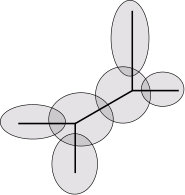 Figure 1
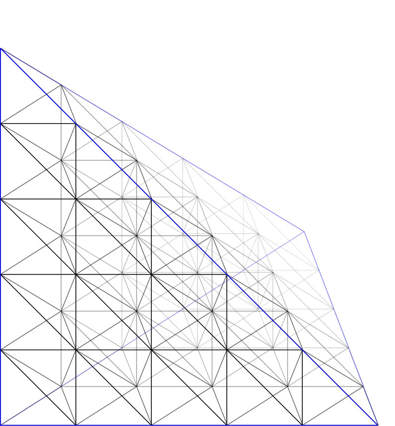 Figure 2
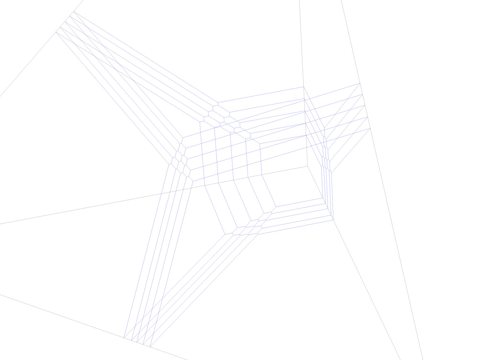 Figure 3
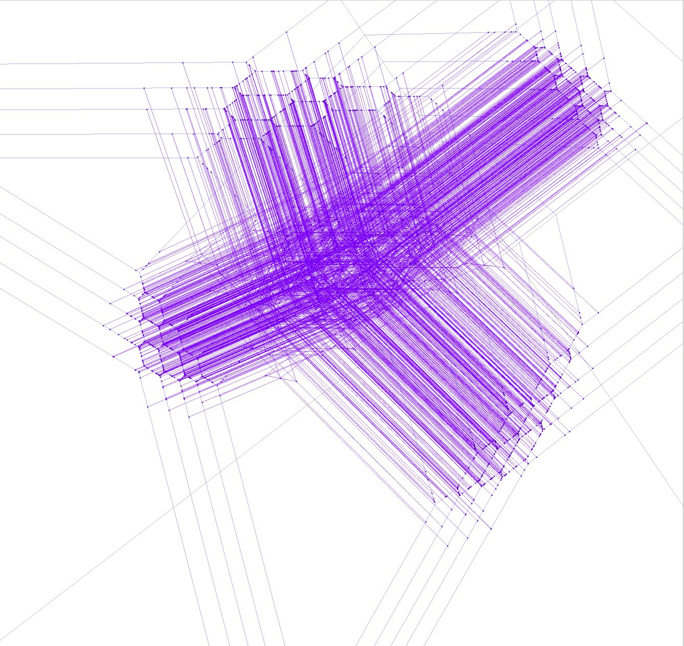 Figure 4
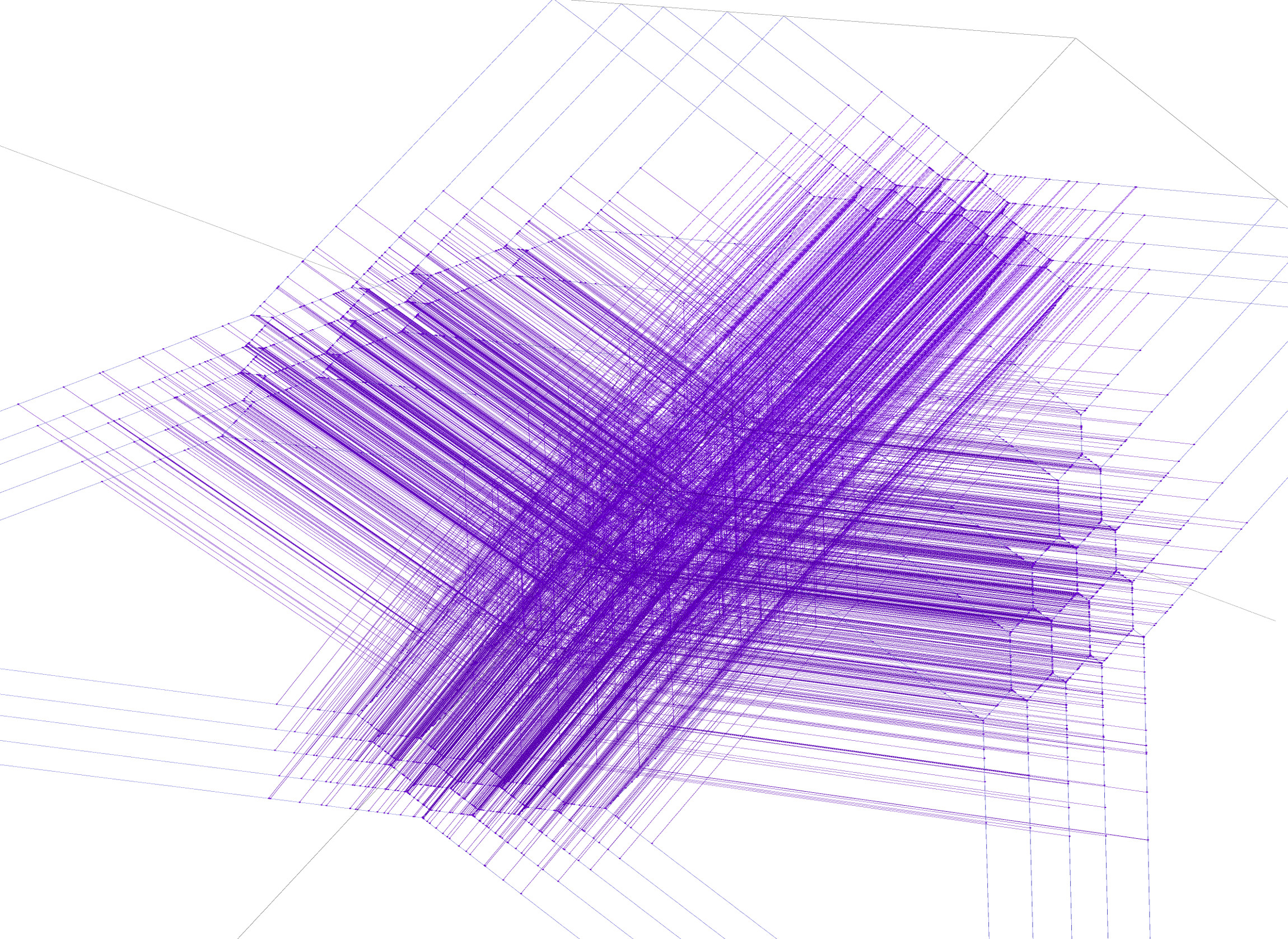 Figure 5
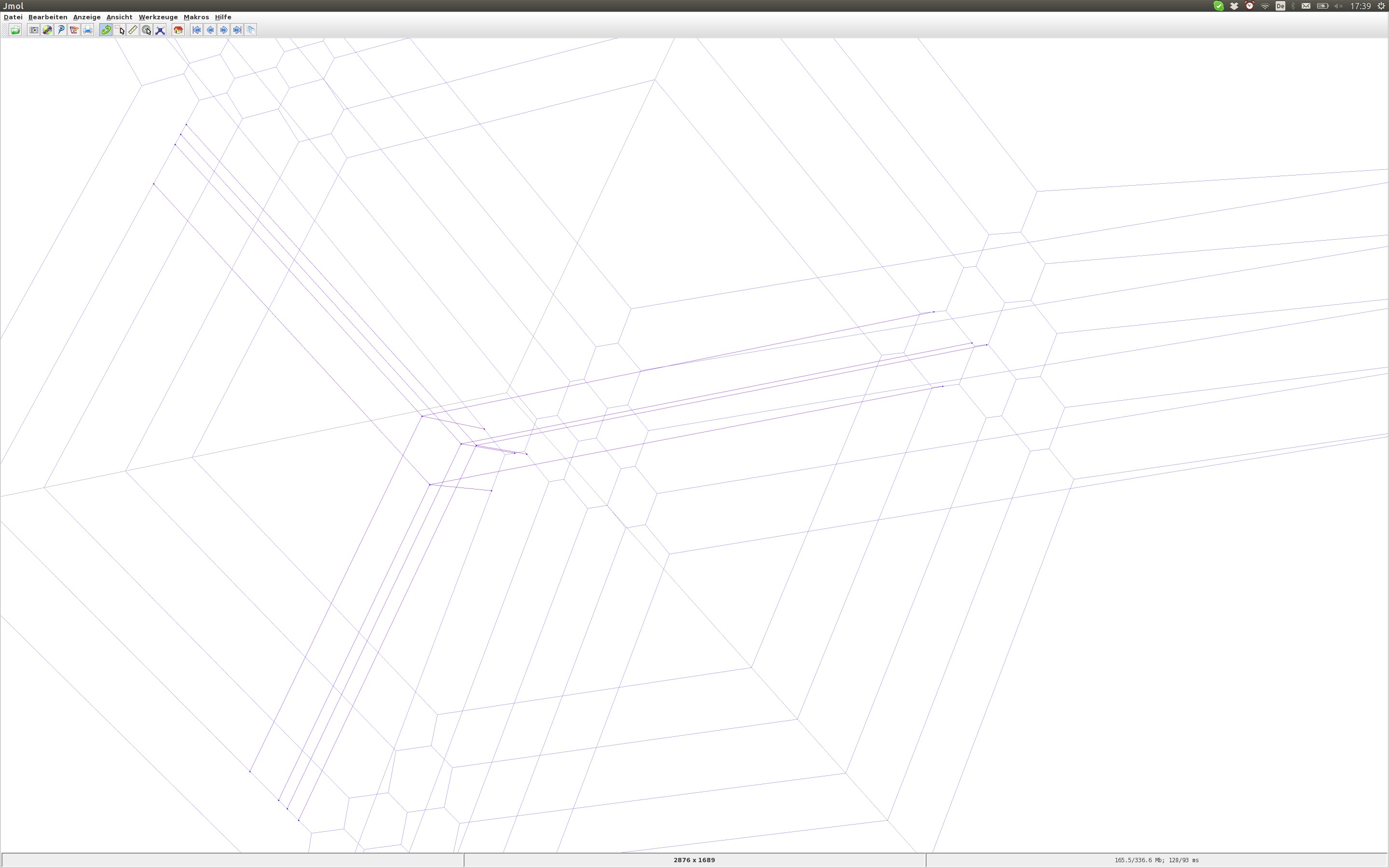 Figure 6
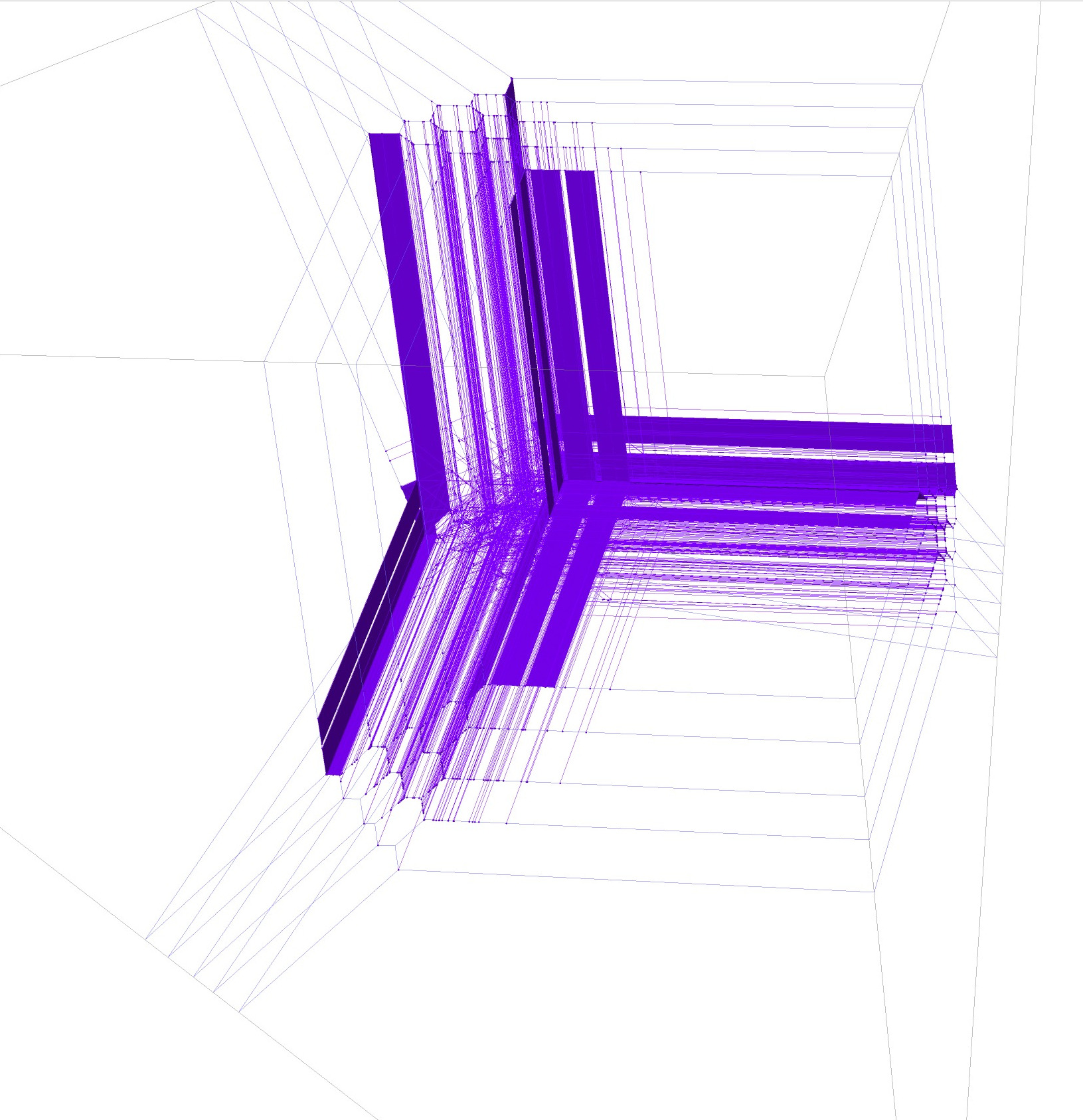 Figure 7
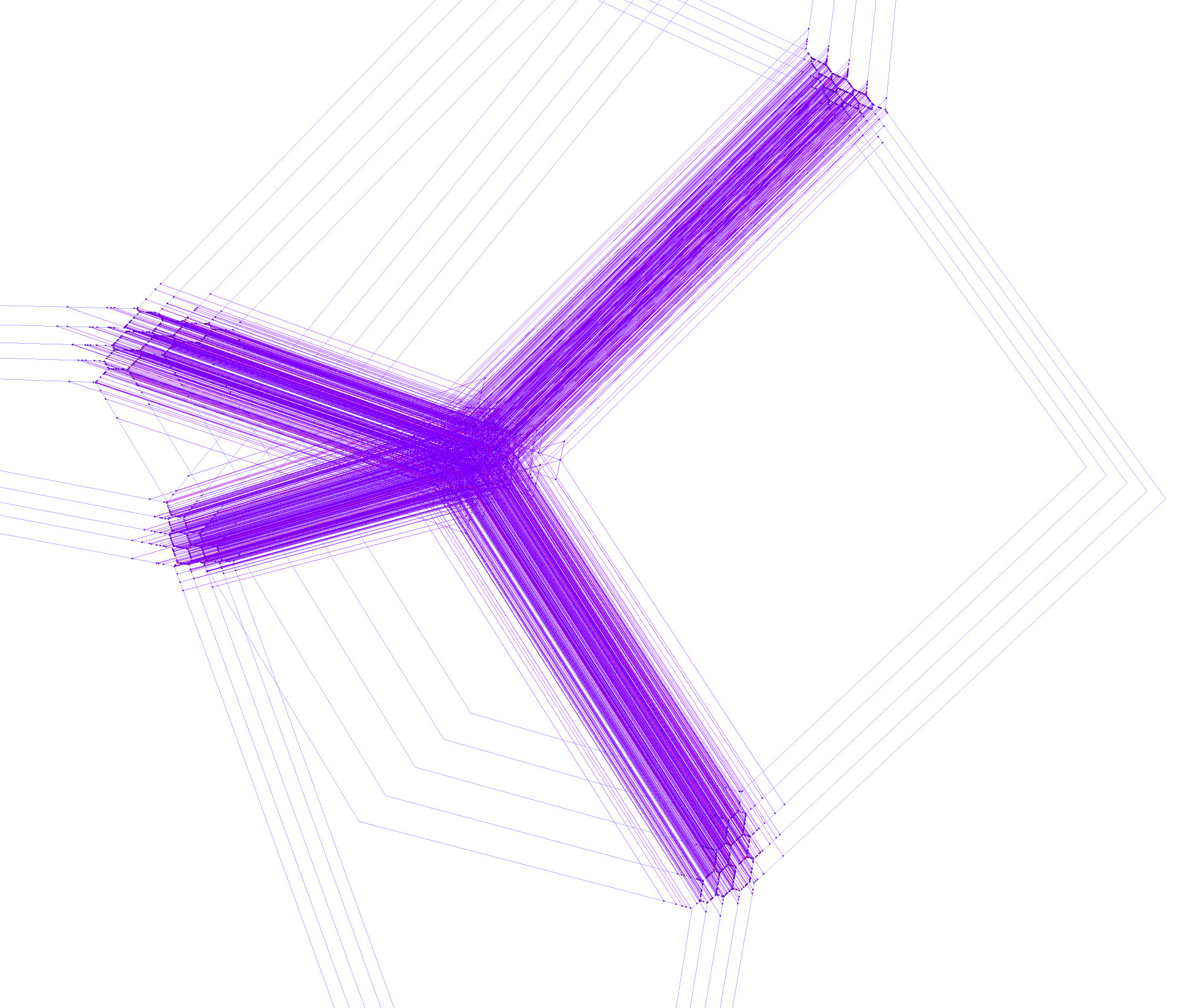 Figure 8
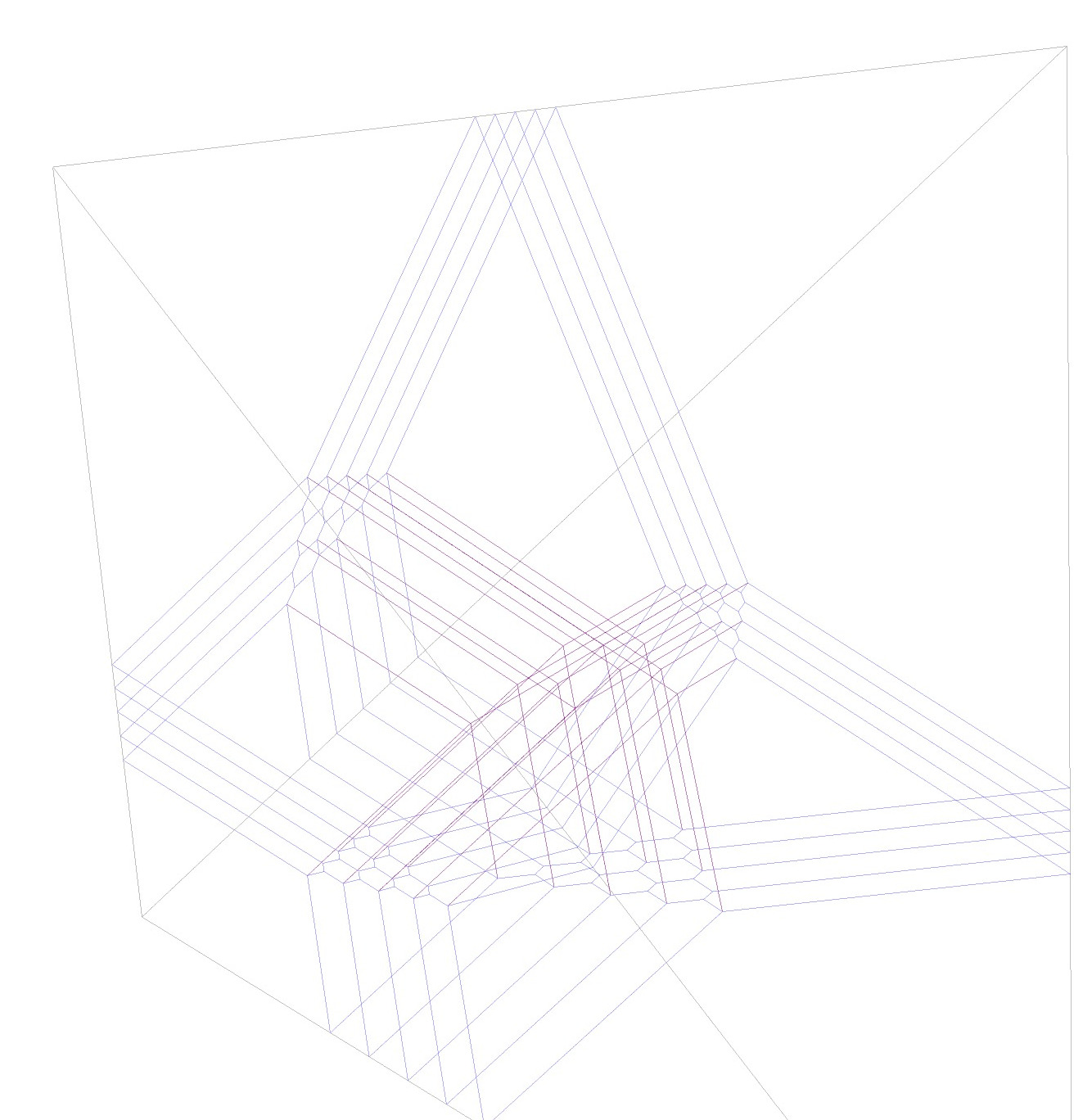 Figure 9
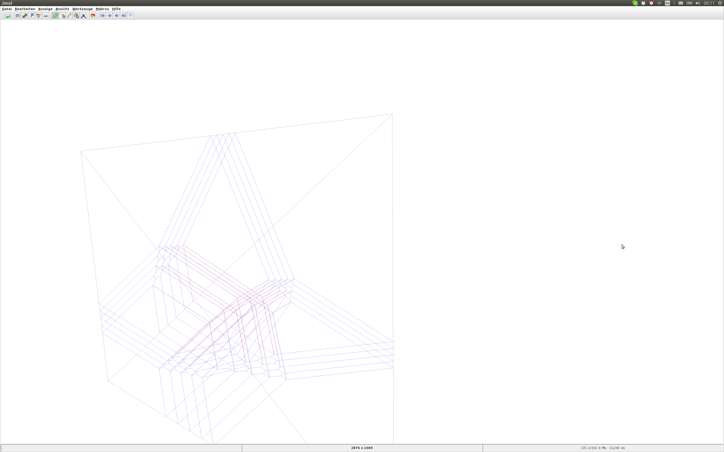 Figure 10
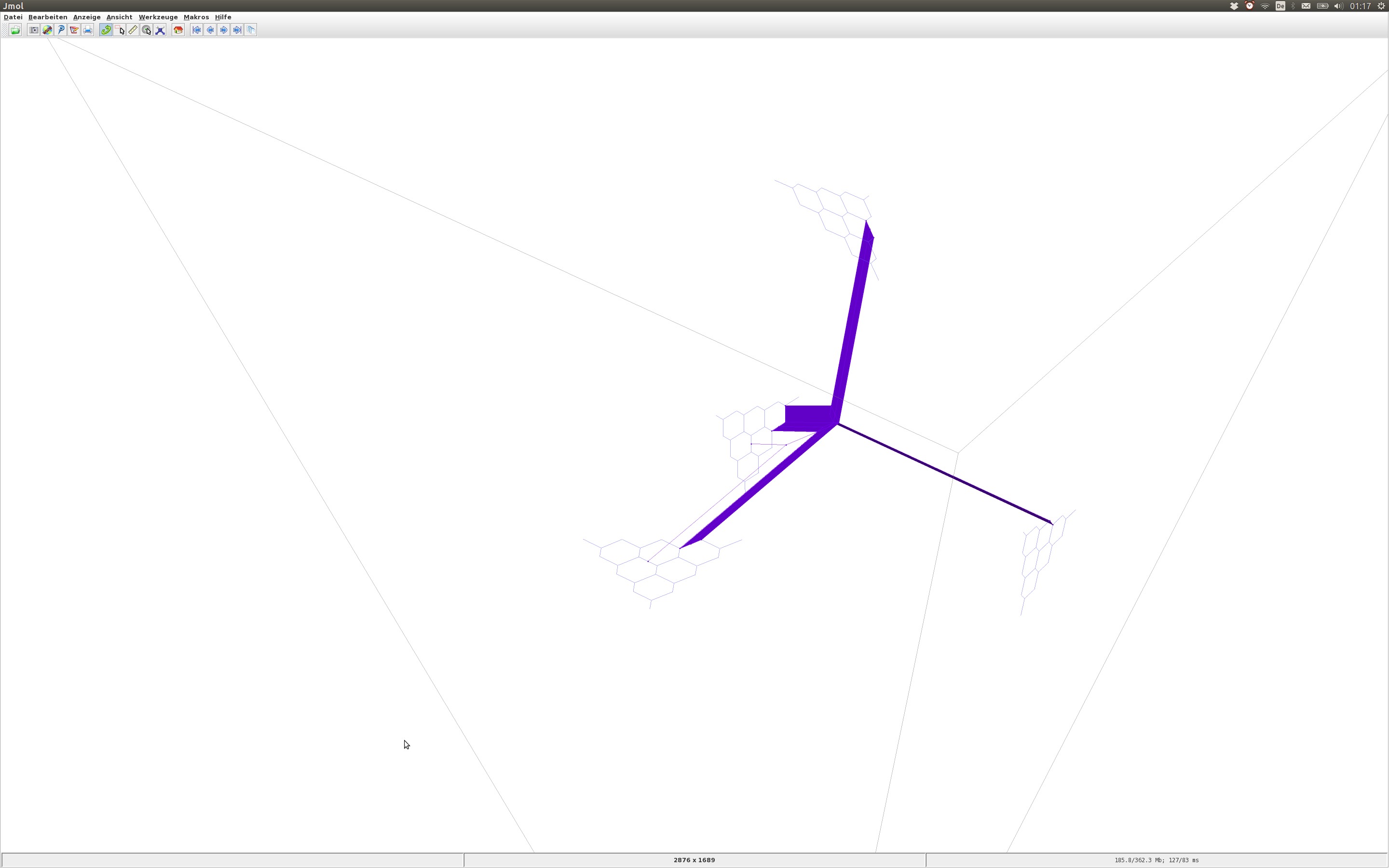 Figure 11
 Figure 12
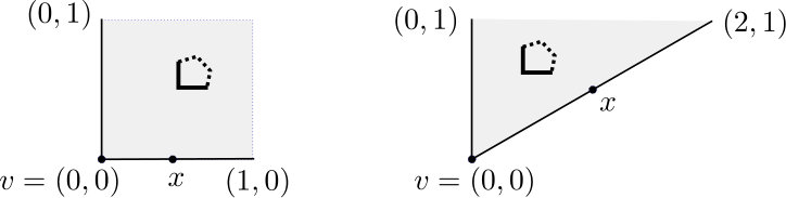 Figure 13
 Figure 14
 Figure 15
 Figure 16
 Figure 17
 Figure 18
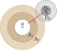 Figure 19
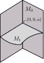 Figure 20
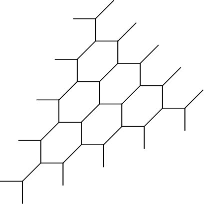 Figure 21
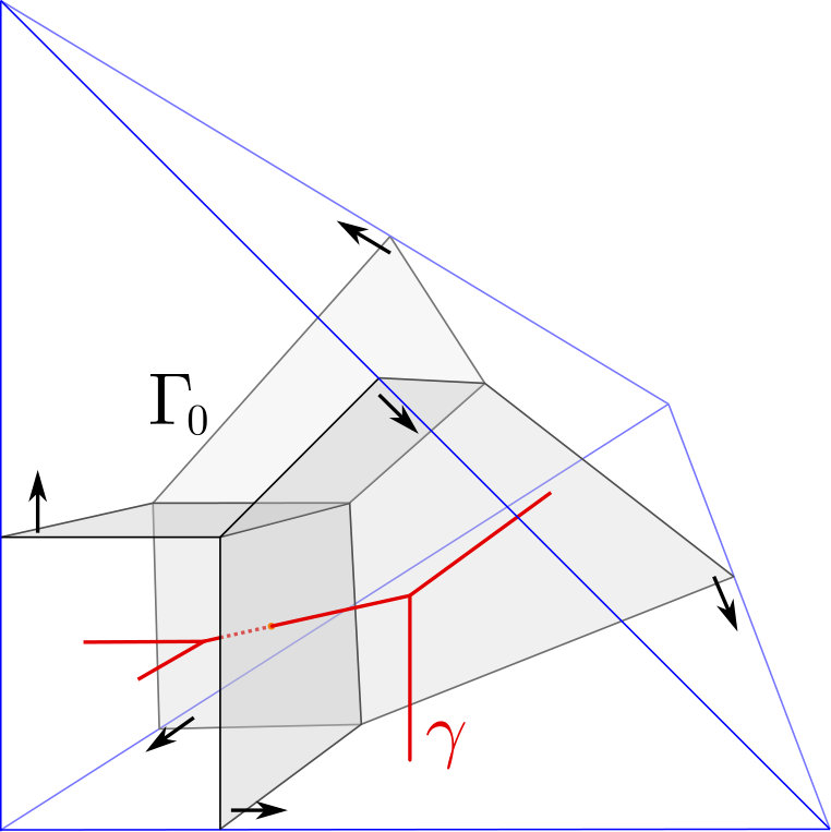 Figure 22
Peer Reviews
No public reviews on file for this paper yet. If you reviewed it on a platform where reviews are public (OpenReview, ICLR, NeurIPS, ICML), you can paste yours below so the community can read it here.
Videos
No videos yet. Explain this paper in a talk, walkthrough, or lecture? Add one.
Tropically constructed Lagrangians in mirror quintic threefolds
Cheuk Yu Mak and Helge Ruddat
JGU Mainz, Institut für Mathematik, Staudingerweg 9, 55099 Mainz, Germany
DPMMS, University of Cambridge, CB3 0WB, UK
Abstract.
We use tropical curves and toric degeneration techniques to construct closed embedded Lagrangian rational homology spheres in a lot of Calabi-Yau threefolds. The homology spheres are mirror dual to the holomorphic curves contributing to the GW invariants. In view of Joyce’s conjecture, these Lagrangians are expected to have special Lagrangian representatives and hence solve a special Lagrangian enumerative problem in Calabi-Yau threefolds.
We apply this construction to the tropical curves obtained from the 2875 lines on the quintic Calabi-Yau threefold. Each admissible tropical curve gives a Lagrangian rational homology sphere in the corresponding mirror quintic threefold and the Joyce’s weight of each of these Lagrangians equals to the multiplicity of the corresponding tropical curve.
As applications, we show that disjoint curves give pairwise homologous but non-Hamiltonian isotopic Lagrangians and we check in an example that mutually disjoint curves (and hence Lagrangians) arise. Dehn twists along these Lagrangians generate an abelian subgroup of the symplectic mapping class group with that rank.
Contents
- 1 Introduction
- 2 From 2875 lines on the quintic to Lagrangians in the quintic mirror
- 3 Toric geometry in symplectic coordinates
- 4 Geometric setup
- 5 Away from discriminant
- 6 Near the discriminant
1. Introduction
Special Lagrangian submanifolds of Calabi-Yau threefolds have received much attention due to their role in mirror symmetry. Based on Thomas and Yau [57], [58], Dominic Joyce [31] conjectured that a Lagrangian submanifold admits a special Lagrangian representative (after surgery at a discrete set of times under Lagrangian mean curvature flow) if is a stable object in the derived Fukaya category with respect to an appropriate Bridgeland stability condition. Therefore, roughly speaking, special Lagrangians correspond to stable objects. In [29], Joyce proposed a counting invariant for rigid special Lagrangians (i.e. special Lagrangian rational homology spheres) so that each of these Lagrangians is weighted by when it is counted and, under the conjectural correspondence between special Lagrangians and stable objects, Joyce’s counting invariant is conjectured to be mirror to the Donaldson-Thomas invariant. One possible explanation of the weight is that objects in the Fukaya category are Lagrangians with local systems and is exactly the number of rank one local systems on , giving many different objects in the Fukaya category. (The original explanation in [29] is different.)
Even before counting, finding special Lagrangians is a challenging problem ([28], [30] etc). The main source of examples is given by the set of real points. Making a given Lagrangian special is hard. Even without the specialty assumption, there aren’t many explicit methods to construct closed embedded Lagrangian submanifolds in Calabi-Yau threefolds in the literature, especially when the Calabi-Yau is assumed to be compact and the Lagrangians spherical. In this paper, we provide a new method to address the latter difficulty using toric degeneration techniques and tropical curves.
The Lagrangians are constructed by dualizing tropical curves that contribute to the Gromov-Witten invariant of the mirror. Therefore, even though we do not show that the Lagrangians we construct are (Hamiltonian isotopic to) special Lagrangians, their quasi-isomorphism classes in the Fukaya category are conjecturally mirror dual to the stable sheaves contributing to the Donaldson-Thomas invariants (via DT/GW correspondence). It is expected that these Lagrangians would give the full set of stable objects in a fixed -class in the Fukaya category with respect to a stability condition, and hence play an important role towards the enumerative study of stable objects in the Fukaya category. In particular, we find that the weight indeed coincides with the multiplicity of the corresponding tropical curve which is also how it enters the mirror dual Gromov-Witten count. We had communicated this result to Mikhalkin who then also confirmed it in his approach [41].
The idea of construction is motivated by Strominger-Yau-Zaslow’s (SYZ) conjecture [56] and the construction of cycles in [50]. Parallel results without connection to enumerative geometry have very recently been achieved independent from us in the situation where the symplectic manifold is non-compact [38], [37], [25, 26], a toric variety [41], [27] or a torus bundle over torus [54].
Roughly speaking, if there is a Lagrangian torus fibration for a Calabi-Yau manifold and a tropical curve in the base integral affine manifold such that all edges of have weight one, then it is easy to construct for each edge of , a Lagrangian torus times interval lying above and for each trivalent vertex of , a Lagrangian pairs of pants times torus lying above a small neighborhood of . Moreover, these local pieces can be constructed in a way that can be patched together smoothly, resulting in a Lagrangian submanifold . Furthermore, if hits the discriminant at the end points appropriately, then can be closed up to a closed embedded Lagrangian , whose diffeomorphism type is determined by the combinatorial type of and the local monodromy at points where the discriminant is hit. We will explain this in more details in Section 2.6. We call a tropical Lagrangian over . The key point is that, this construction is straightforward only when we have been given a Lagrangian torus fibration. However, the only compact Kähler Calabi-Yau threefolds that knowingly admit a Lagrangian torus fibration are torus bundles over a torus.
Our actual construction starts with a family of smooth threefold hypersurfaces in a toric -orbifold degenerating to , the toric boundary divisor of with the reduced scheme structure. Let be the locus of singular points of , , be the discriminant, be the moment map and . Suppose that has at worst isolated Gorenstein orbifold singularities. The singularities are necessarily at the preimage of vertices of under , and thus is a smooth threefold for small.
Starting with a reflexive polytope , [21] exhibited a Minkowski summand so that has the property that is simple ([23], Definition 1.60). We equip with an integral affine structure using the integral affine structure on and the fan structure at the vertices, see Definition 3.13 in [21], Example 1.18 in [23]. Therefore, we can define tropical curves in , see Definition 2.2 below. We require to be the set of univalent vertices of . Let be the local system of integral tangent vectors on . When is rigid and is trivializable over , we can associate to its multiplicity defined in [35] (cf. [36],[42]), which we recall in Section 2.7. The multiplicity depends on the directions of edges of as well as the monodromy action around near the univalent vertices of . We call a tropical curve admissible if for each univalent vertex , there is a neighborhood of such that is an embedded curve (rather than two-dimensional). The tropical lines that end on the “internal edges of the quintic curves” in a mirror quintic threefold are admissible, see Lemma 2.6 – in the example of Section 2.5, more than half of the lines are admissible. Moreover, an admissible tropical curve determines a diffeomorphism type of a -manifold in the way that the diffeomorphism type of a tropical Lagrangian over is determined by . By slight abuse of terminology, we call the diffeomorphism type determined by a Lagrangian lift of (see Section 2.6). We denote the -neighborhood of with respect to the Euclidean distance on by . Our main theorem is:
Theorem 1.1**.**
Let be an admissible tropical curve in . For any , there exist a such that for all , there is a closed embedded Lagrangian such that and is diffeomorphic to a Lagrangian lift of . Moreover, whenever is well-defined, we have .
Remark 1.2*.*
For discussion of non-admissible tropical curves, see Remark 6.3, 6.21.
Remark 1.3*.*
While our main examples are mirror quintics, Theorem 1.1 applies to all admissible tropical curves that arise from the setup in [21] explained above. For example, the tropical curves are not necessarily simply connected.
Remark 1.4*.*
While is only defined when is trivializable over [35], in view of Theorem 1.1, it is tempting to define by when is not trivializable. We believe that this definition will have application to enumerative problems in algebraic/tropical geometry.
Remark 1.5*.*
One can easily generalize to all dimensions (see Remark 2.10). However, it is pointed out to us by Joyce that we do not expect a special Lagrangian counting invariant in dimensions higher than .
Sketch of proof of Theorem 1.1.
The construction is divided into two parts: for the geometry away from the discriminant and near the discriminant. Both constructions rely heavily on the fact we can isotope symplectically to a nice symplectic hypersurface in local coordinates, as long as the isotopy is away from the discriminant and does not produce new discriminant (see Lemma 4.1).
For the construction away from the discriminant, we isotope to a standard form (Lemma 5.4) in a chart such that admits a local Lagrangian torus fibration and we can construct a local Lagrangian from the torus fibration (Proposition 5.5). We have to deal with compatibility of standard forms (Lemma 5.11), transition of symplectic charts (Corollary 5.15) and the trivalent vertices of (Lemma 5.19). The outcome will be an embedded Lagrangian with toroidal boundaries such that the -image lies in a small neighborhood of .
Then we need to close up the Lagrangian with toroidal boundaries by Lagrangian solid tori near the discriminant, which is the essential part of the construction. The basic idea is that we can deform to a particular such that we have complete control away from the discriminant. We find an appropriate open subset of which is an exact symplectic manifold with contact boundary (Proposition 6.29) and we have complete control near the contact boundary of . We show that is a symplectic bundle over an annulus and we use our control near to show that the boundaries of the fibers are standard contact . By a famous result of Gromov, each fiber is symplectomorphic to an open -ball (Theorem 6.8). There is a Legendrian inside , which is an -bundle over with respect to the symplectic -ball fiber bundle structure on . This Legendrian can be filled by a Lagrangian solid torus in by a soft symplectic method (Proposition 6.19), which gives the Lagrangian solid torus we need.
Once the Lagrangian is constructed, the statement that follows from a simple calculation using Čech cohomology (see Subsection 2.7) which was independently obtained in [41] by a different argument after a presentation of our result given by the second author in 2017. ∎
Application to symplectic topology
Let be the set of admissible tropical lines in associated to a pencil of mirror quintics. We can show that the Lagrangians constructed by Theorem 1.1 are homologous and non-Hamiltonian isotopic in the following sense:
Theorem 1.6**.**
Let and be a Lagrangian obtained by Theorem 1.1. For any , we can get a Lagrangian by Theorem 1.1 such that . Moreover, if , then is not Hamiltonian isotopic to .
Theorem 1.6 gives a large number of pairwise homologous but non-Hamiltonian isotopic Lagrangian rational homology spheres, which is a rare application to symplectic topology in the literature.
When is diffeomorphic to a free quotient of a sphere by a finite subgroup of , we can define Dehn twist along , which is an element in the symplectomorphism group of . It is easy to deduce from Theorem 1.1 the following:
Corollary 1.7**.**
Let be the maximum number of disjoint tropical curves satisfying Theorem 1.1 such that for each , the corresponding is a spherical manifold. Then contains an abelian subgroup isomorphic to .
Note that, in generic situations, most tropical curves are disjoint from the others so Corollary 1.7 gives a large rank of abelian subgroup in .
By a computer-aided search for a particular symplectic mirror quintic, we found pairwise disjoint admissible tropical lines giving Lagrangian and Lagrangian in the mirror quintic all of which are pairwise disjoint. The total number of admissible tropical lines in our example is out of which have multiplicity one (giving Lagrangian ’s) and have multiplicity two (giving Lagrangian ’s). The total number of tropical lines in our example is however out of which have multiplicity one and have multiplicity two, so the weighted sum is indeed 2875. Their adjacency matrix has full rank, which implies that every tropical line intersects some other tropical line. Inspection of the center of Figure 2.3 gives an impression of the meeting of tropical lines, yet tropical lines also meet another across components of the degenerate Calabi-Yau unlike possibly expected. We don’t know whether this is a general phenomenon or due to possibly not having picked the most general deformation. We chose a random small perturbation of the subdivision given in Section 2.4.
Structure of the paper
In Section 2 we give some background of SYZ mirror symmetry and the tropical curves in the affine base. We also explain the topology of the Lagrangians and derive some consequences, including Theorem 1.6, by assuming Theorem 1.1, which is proved in the subsequent sections. In Section 3, we review toric geometry from symplectic perspective. In Section 4, we explain how to perform symplectic isotopy away from the discriminant for our pencil of hypersurfaces. After that, we explain the construction of the Lagrangians away from the discriminant and near the discriminant in Section 5 and 6, respectively. We conclude the proof of Theorem 1.1 in Section 6.8.
Acknowledgments
We thank Paul Seidel for suggesting to study mirror duals of lines and for bringing the authors together at the Institute for Advanced Study in Princeton. Further thanks for helpful discussions goes to Mohammed Abouzaid, Ivan Smith, Travis Mandel, Johannes Walcher, Hans Jockers and Penka Georgieva. We also thank the two anonymous referees.
The first author was funded by National Science Foundation under agreement No. DMS-1128155 and by EPSRC (Establish Career Fellowship EP/N01815X/1). The second author was funded by DFG grant RU 1629/4-1. The authors thank the support of Hausdorff Research Institute for Mathematics (Bonn), through the Junior Trimester Program on Symplectic Geometry and Representation Theory.
2. From 2875 lines on the quintic to Lagrangians in the quintic mirror
The toy model of the SYZ mirror symmetry conjecture is the following. Set and let and denote the tangent and cotangent bundle. Let denote the local system on of integral tangent vectors (using the lattice in ). The quotient is an -bundle over . Similarly, we can define and another -bundle . We arrive at dual torus fibrations over ,
[TABLE]
where the left one carries a natural complex structure with complex coordinates given by and the th coordinate on . The right one carries a natural symplectic structure inherited from the canonical one of . Part of the conjecture of SYZ is that mirror symmetry is locally of this form. Unless talking about complex tori, in practice there are also singular torus fibers in these bundles for Euler characteristic reasons and we will get back to this.
Note that this toy model gives insight on how a complex submanifold ought to become a Lagrangian submanifold of the mirror dual (see Section 6.3 of [3]). If is an integrally generated linear subspace of , then is naturally a complex submanifold of . On the other hand, as a subbundle of supported over is a Lagrangian submanifold of . To reach sufficient generality, one needs to run this construction for the situation where is a tropical variety, i.e. a polyhedral complex. At a general point it still looks just like the above but then pieces are glued non-trivially when polyhedral parts meet another. However, this doesn’t produce a differentiable submanifold, let alone complex or Lagrangian. Improvements on the symplectic side can be made by thickening the tropical to an amoeba, see [37]. In this article, we are only interested in the situation where is one-dimensional, so a tropical curve, and the focus will be put on constructing closed Lagrangian submanifolds in Calabi-Yau threefolds using tropical curves. Whenever compactifies to a projective toric variety and the tropical curve attaches to the codimension two strata in the moment polytope in particular ways, Mikhalkin recently gave a construction of closed Lagrangian submanifolds in the projective toric variety [41]. On the other hand, no Lagrangian torus fibration is known for any simply-connected compact Calabi-Yau threefold. This is the situation that we are interested in, which is also the subject of the SYZ conjecture. Luckily, most Calabi-Yau threefolds permit degenerations to a reducible union of toric varieties, introducing the toric techniques we lay out for the quintic and its mirror dual in the next sections.
2.1. The quintic threefold and its symplectic mirror duals
The most famous Calabi-Yau threefold is the quintic in . Its mirror dual is a crepant resolution of an anti-canonical hypersurface in the weighted projective space associated to the lattice simplex
[TABLE]
One finds . As progress towards nailing the SYZ conjecture for the quintic, Mark Gross [20, Theorem 4.4] gave a topological torus fibration on a space that is diffeomorphic to and Matessi and Castaño-Bernard [6] showed that this one can be upgraded to a piecewise smooth Lagrangian fibration for some symplectic structure and a similar approach works for . Recently, Evans-Mauri [15] gave a Lagrangian fibration local model for parts of the fibration that are most difficult to deal with in dimension three. Whether this can be used for global compactifications of fibrations or tropical Lagrangian attachment problems presumably requires a similarly careful analysis as for the situations that we are going to consider. For recent progress on the SYZ topology, we refer to [46, 45, 47].
We are not working on the diffeomorphic model but on the actual symplectic quintic mirror , in fact our construction applies to Lagrangians in each of the many possibilities resulting from different choices of a crepant resolution for the quintic mirror (). For our construction, it suffices to have a Lagrangian torus fibration locally around the Lagrangian that we wish to construct from a tropical curve . To say where lives, we make use of the construction of the real affine base space of the torus fibration from [20].
The Newton polytope of the quintic is the polar dual to , that is, the convex hull translated by so that its unique interior lattice point becomes the origin. We call the resulting polytope . Choosing for each yields a cone in generated by the set of and its boundary gives the graph of a piecewise linear convex function . We require that every face in the boundary is a simplicial cone and we assume that each generates a ray of this cone, in particular, for all . There are lots of satisfying these properties and each one gives a toric projective crepant partial resolution
[TABLE]
where is given by the fan in whose maximal cones are the maximal regions of linearity of . Equivalently, is given by the polytope
[TABLE]
Lemma 2.1**.**
* has at worst isolated Gorenstein orbifold singularities.*
Proof.
If is a maximal cone in the fan, i.e. a maximal region of linearity of , then it is simplicial by assumption, hence generated by say. Moreover, these generators are all contained in a single facet of because the fan refines the normal fan of . By the assumption that each for is a ray generator, we find . So is a cone over the elementary lattice simplex given by the convex hull of , thus gives a terminal toric Gorenstein orbifold singularity and these have codimension four. ∎
Let be the monomial associated to . Consider the (singular) hypersurface in given by an anti-canonical section written as a Laurent polynomial on ,
[TABLE]
with and (so that gives a submanifold of , cf. [4, §2]). The monomial exponents of are precisely the lattice points of . The closure of in misses the isolated orbifold points at zero-dimensional strata (Lemma 2.1) and gives a symplectic -manifold with symplectic structure induced from . Furthermore, is a Calabi-Yau manifold as it agrees with the crepant resolution under of the anti-canonical hypersurface, the closure of inside . By deforming the , one can study continuous deformations of the symplectic structure. The space of crepant symplectic resolutions acquires an interesting chamber structure with a point on a wall given by a set of that violates the simplicialness of . Just as a remark: the wall geometry is governed by the secondary polytope of .
2.2. The real affine manifold and tropical curves
Following [21], we next explain how to give a real integral affine structure on a large open subset of where is a lattice polytope obtained from a as in Section 2.1. We split as a Minkowski sum
[TABLE]
where is the polytope associated to the piecewise linear function that takes value at . Indeed, this gives a decomposition as claimed because is the polytope of the function taking value on all of , so . By the decomposition, every vertex of is uniquely expressible as for a vertex of and a vertex of . We project a small neighborhood of onto the quotient of the affine four-space that contains by the affine line resulting an affine three-space. The projection is thus injective and thereby gives a real affine chart for . There is also an integral structure obtained by complementing to a lattice basis of to find a lattice for the quotient. We do this for each vertex of . Furthermore, for each facet of , its interior carries a natural integral affine structure from the tangent space to the facet. Combining the resulting charts with the interiors of facet yields an atlas on the union of these charts for an integral affine structure, i.e. transitions in . By choosing suitably, the complement of the union of charts can be made to be
[TABLE]
where is the union of complex two-dimensional strata, the union of two-cells of and is the moment map for the Hamiltonian -action on . We don’t need to be a lattice polytope for this construction. The affine structure is integral affine because is a lattice polytope. Let denote the local system of integral tangent vectors on (we also used before).
Definition 2.2**.**
A tropical curve in is a graph (realized as a topological space) together with a continuous injection such that
- (1)
a vertex of is either univalent or trivalent, 2. (2)
is a univalent vertex of , 3. (3)
the image of the interior of an edge is a straight line segment in the affine structure of of rational tangent direction, 4. (4)
For with , the primitive tangent vector of the adjacent edge generates the image of for the monodromy of along any non-trivial simple loop around in a small neighborhood of . 5. (5)
For every trivalent vertex , and the primitive tangent vectors into the outgoing edges, we have and span a saturated sublattice of .
We consider two tropical curves the same if there exists a homeomorphism that commutes with . By slight abuse of notation, we also use to refer to the image of . The following lemma guarantees that we can always satisfy (4) above as long as the tropical curve approaches from the right direction. The lemma directly follows from the aforementioned simplicity of , c.f. [20].
Lemma 2.3**.**
Let be a point contained in a small neighborhood so that is homotopic to as a pair, where is an open disc and is a point in . Let be a generator and the monodromy of along . In a suitable basis of , is given by . In particular, the image of is saturated of rank one, i.e. generated by a primitive vector.
2.3. Katz’s methods for finding lines on a quintic
The quintic permits a flat degeneration to the union of coordinate hyperplanes simply by interpolation. If is given by the homogeneous quintic equation in the variables then we define the family of hypersurfaces in varying with by
[TABLE]
and denote by the fiber with . Since is the union of five projective spaces, it contains infinitely many lines. However, only a finite number of them deforms to the nearby fibers, worked out by Katz in [53]. Assuming is general, the intersection of with each coordinate two-plane is a smooth complex quintic curve. There are ten of these.
Theorem 2.4** (Katz).**
A line in deforms into the nearby fiber if and only if it does not meet any coordinate line of but meets four of the quintic curves.
Note that it follows that a line which deforms needs to be contained in a unique irreducible component of and needs to meet the quintic curves that are contained in this component, namely the intersections of the four coordinate planes of with . A general quintic hosts many lines and in the degeneration, each contains deformable lines, [53]. On the dense algebraic torus of , we may apply the map given by for each coordinate. Each line maps to an amoeba with four legs going off to infinity in the directions of the rays in the fan of the toric variety . Furthermore, these legs “meet the amoeba of the quintic plane curves at infinity”. We are not going to make this more precise because we only use this idea as inspiration. There is a closely related theorem that was our main motivation combined with Katz’s findings:
Theorem 2.5** ([35]).**
The number of tropical lines in meeting general quintic tropical curves at tropical infinity each in one of the four directions of the rays of the fan of when counted with their tropical multiplicities agrees with the number of complex lines in meeting five general quintic plane curves.
So we may almost deduce from Katz’s count of complex lines a count of tropical lines via this theorem. The only issue here is the attribute “general”. Indeed, the quintic curves in Katz’s situation are not in general position. If they were, the count would be by standard Schubert calculus but this number is way bigger than . Indeed, any pair of quintic curves meets each other in points which wouldn’t happen if they were in general position. They meet each other because they arise from the same equation restricted to each coordinate plane.
We expect that in the more special position where the tropical quintics meet each other, after removing degenerate tropical lines (meaning those that move in positive-dimensional families, meet vertices of the discriminant curve or don’t have the expected combinatorial type ), then one actually finds when counting these with multiplicity. We verify this below in a global example. Before going into its details, let us clarify why tropical lines in that meet tropical quintics at infinity relate to in the sense of Definition 2.2. For , setting , we observe and . In this sense, is a deformation of and note that has the same combinatorial type for all . Recall the notion of the discrete Legendre transform from [22, 23, 49]. Since and are polar duals, their boundaries are discrete Legendre dual, [23, Example 1.18]. The subdivided boundary of by means of is the discrete Legendre dual to . For a -cell in , there are three possibilities for what its deformation in can be, namely [math]-, - or -dimensional. These cases match with whether its dual (one-dimensional) face in the subdivision of lies in a -, - or -cell of . Most importantly, since the subdivision of by governs the composition , the following holds.
Lemma 2.6**.**
Let be a -cell. Recall the monomials . We set and means that the vertex of corresponding to is contained in . The amoeba part is given by
[TABLE]
as an equation on the torus orbit dense in the stratum of given by .
In particular, for deforming to an edge of , is a binomial. Also note that if is a [math]-cell.
Note that is a binomial if and only if the corresponding amoeba is one-dimensional and hence tropical curves ending on it will be admissible (see also Remark 6.2).
If is a unimodular subdivision, e.g. as in Figure 2.2, then most two-cells of have , there are many two-cells of that deform to triangles in but most interestingly for us, two-cells deform to edges, hence their amoeba is given by a binomial. These amoeba pieces arrange as plane quintic curves, e.g. as in Figure 2.1. (One verifies that indeed the number of interior edges is here.) Each quintic curve is dual to the triangulation of a two-face of , e.g. consider the front face in the right hand part of Figure 2.2. Each facet of contains four triangle faces,
hence dually, four quintic curves arrange together as the boundary of a space tropical quintic surface in . In particular, we can view them as lying at infinity and since they make up the discriminant in , a tropical line in with ends on the four quintics thus gives a tropical curve in . There are a lot of these, see Figure 2.3 and most of them are admissible, i.e. they meet one of the 30 inner edges of each quintic, rather than the outer ones. Also note that this configuration appears five times in the boundary of .
2.4. A very symmetric subdivision and resolution of the quintic mirror
We next give an example for that is even a manifold, see also [20, p. 122: Fig. 4.6]. The subdivision of each facet of is obtained from the affine Weyl chambers of type , cf. [32, III,§2]. Concretely, let be the unique continuous convex function that is linear on each connected component of , changes slope by at each point in and is constantly zero on , see Figure 2.2. One finds for (“discrete parabola”). Now consider the piecewise affine function given by
[TABLE]
and finally define as the unique piecewise linear function on that coincide with on . For , set and recall from Section 2.1 that is entirely determined from the set of .
The induced subdivisions of any two facets are isomorphic and looks like what is on the right in Figure 2.2. One checks that each four-dimensional cone in the fan given by is lattice-isomorphic to the standard cone , so the resulting is smooth. In our explicit example below, we will use a slight perturbation replacing by for random to increase our chance of being in a generic situation. Plugging the perturbed into (2.1) yields a slightly deformed and while the complex manifold doesn’t change, as this slightly perturbs the symplectic form in a well-understood manner. The best way to understand what looks like is by considering its discrete Legendre dual. The subdivision of by is five copies of the right hand side of Figure 2.2 glued along facets. Therefore, after identification there are ten -faces, each carrying a subdivision that is dual to that of a quintic curve in its most symmetric form show in Figure 2.1.
2.5. The findings of a computer search for the tropical lines
As described in the previous section, we obtained a particular as a small perturbation of that gave the very symmetric subdivision of . From Katz’s work as described in Section 2.3, we are looking for tropical lines in that meet the quadruple of tropical quintic curves where each tropical quintic is dual to the subdivision of one of the triangle faces of . We used a computer for this search following the pseudo code111For more details, the complete code with instructions and results, see
https://www.staff.uni-mainz.de/ruddat/lines-in-quintic/lines.html or look at the ancillary files of this third arxiv version.
After removing all lines that meet vertices of the quintics, that have only one internal vertex or are non-rigid (that is move in families), we did actually get the expected count — when counting with multiplicity (which is remarkable in view of [60, 44, 8]). That is, maybe surprisingly, the lines weren’t all of multiplicity one. We give the definition of the multiplicity in Section 2.7. For each of the five facets of , the count with multiplicity of the tropical curves gave indeed , so in total as expected. We found curves of multiplicity one and of multiplicity two. These did not evenly distribute over the facets: . While is a number that hasn’t appeared yet in the context of the quintic to our knowledge, one may speculate that relates to the count of real lines that was found to be in [55]: for rational curves on an elliptic surface, the presence of higher multiplicity tropical curves is implied from the Welschinger invariant to differ from the Gromov-Witten invariant, see e.g. [59, §4.2.2].
The goal is to construct Lagrangian threefolds from these tropical curves. The remainder of this article carries this out for admissible curves. Recall that the requirement is that the tropical curve meets the discriminant amoeba in points where this amoeba is one-dimensional. By Lemma 2.6, this holds true if the tropical line meets the internal edges of the quintic curves, i.e. no outer edges. A bit more than half the curves feature this: we get admissible lines out of which have multiplicity two (multiplicity weighted account is ). Interestingly, the admissible curves don’t meet curves of other facets (unlike non-admissible ones), though possibly still other curves in their own facet. We found a set of admissible lines that are pairwise disjoint out of which have multiplicity two.
2.6. Lagrangian lift of a tropical curve
In this section, we give the definition of the diffeomorphism type of a Lagrangian lift of a tropical curve in to the Calabi-Yau given by , e.g. the mirror quintic as before. Using the integral affine structure on , we can define a Lagrangian torus bundle by
[TABLE]
Recall the notation and note that is an orientable topological manifold and so . Fixing an orientation once and for all, we can talk about oriented bases of stalks of .
For each edge of and a point in the interior of , we get the -dimensional subspace of consisting of co-vectors that are perpendicular to the direction of . By Definition 2.2 (3), every translation descends to an embedded -torus in . A smooth family of these 2-tori over defines a (trivial) torus bundle over and the total space is a Lagrangian submanifold in . It extends over the vertices of that don’t lie in , and we let denote the extension.
Remark 2.7*.*
Let be a smooth function such that it descends to a compactly supported function . Given a smooth family of 2-tori over as above, we can define a new family by fiberwise translating the 2-tori by . The resulting Lagrangian is a different embedding of a 2-torus times interval to . The function being compactly supported corresponds to that the two embeddings coincides near the ends of .
For each trivalent vertex of , by Definition 2.2 (5), we can identify the primitive tangent vector of the outgoing edges as , and with respect to a -basis of . Let be the subset of consisting of all the points such that
[TABLE]
Equipping with the subspace topology yields a finite CW complex of the same homotopy type as a pairs of pants times a circle. More explicitly, has a trivial circle factor given by the -coordinate, and (2.3) defines two triangles in the -coordinates and the vertices of the triangles are glued at respectively (see Figure 2.4).
If we equip the two triangles in (2.3) with opposite orientations, then the boundary of them is exactly given by the circles , and . For , the product of with the circle in -coordinate is exactly where and . For an appropriate choice of orientations, one can see that the boundary of cancels the boundary of lying above , yet is only a Lagrangian cell complex instead of a manifold. In Section 5.2, we explain how to replace the union of the triangles by a pairs of pants and obtain a Lagrangian pair of pants times circle that can be glued with smoothly.
Every univalent vertex of lies in by Definition 2.2(2). Let and be as in Definition 2.2(4), so, by Lemma 2.3, for a suitable basis. The primitive direction of the edge adjacent to is by assumption given by so the 2-tori in lying above are generated by . We can glue a solid torus to the toroidal boundary component of lying above to cap off this boundary component. Moreover, we require that the circle generated by is a meridian of . It is useful to observe that is characterized by being perpendicular to the invariant plane .
Definition 2.8**.**
The diffeomorphism type of a Lagrangian lift of a tropical curve is the diffeomorphism type of the closed -manifold obtained by gluing and as above over all vertices and edges of .
2.7. Lagrangian weight versus tropical multiplicity
Following Joyce, we define the weight of a Lagrangian rational homology sphere to be and more generally . Let be a tropical curve in . In this subsection, we explain how of a tropical Lagrangian can be computed by a Čech covering of the corresponding tropical curve . Since our Lagrangian is homotopic to the Lagrangian cell complex that is built by instead of at the trivalent vertices (see Section 2.6), it suffices to compute the first homology of . For simplicity, we denote by in this subsection. The universal coefficient theorem gives , so we may compute via Čech cohomology.
A collection of open sets in that covers is called admissible if
- (1)
whenever are pairwise distinct, 2. (2)
for all , is connected and it contains exactly one vertex of which is, by definition, either trivalent or univalent, and 3. (3)
for , (which may be empty) contains no vertex.
For admissible, and are torsion free for all and therefore
[TABLE]
where the map is the Čech map on (restriction with sign). Recall from [42, 35, 36] the definition of multiplicity of a tropical curve . Applicable for us is [35, Equation (13)] since we need to consider tropical curves with constraints on unbounded edges (i.e. univalent vertices for us). Let be the interior of and assume that we can trivialize on , i.e. set and . Furthermore, each univalent vertex of gives a saturated rank two subspace in as the kernel of near . We view this as a constraint for the tropical curve in in the sense of [35]. Given these constraints, [35, Equation (13)] provides a map of lattices whose cokernel torsion gives the tropical multiplicity of .
Proposition 2.9**.**
The Čech map is quasi-isomorphic to the tropical multiplicity computing map from [35, Equation (13)] and thus .
Proof.
The assertion follows if one shows that there is a natural isomorphism
[TABLE]
whenever and is the primitive generator of the edge of that meets and an isomorphism
[TABLE]
whenever contains a trivalent vertex and an isomorphism
[TABLE]
whenever contains a univalent vertex of , and the primitive generator of the image of . Furthermore the restriction maps are supposed to be the natural maps under these isomorphisms. The isomorphisms and naturality of restriction maps are straightforward to be checked from the local descriptions of and given in Section 2.6. ∎
Remark 2.10*.*
Proposition 2.9 can be generalized to all dimensions for all tropical curves satisfying exactly the same set of conditions in Definition 2.2. The main reason is that, in higher dimensions, and split as a product and there is a trivial factor accounting for the extra dimensions. Moreover, the universal coefficient theorem gives no matter what the dimension is so the same Čech cohomology calculation applies to conclude that .
2.8. Homology class of the Lagrangians
Recall from Section 4 in [48] that a tropical 2-cycle in an affine manifold with singularities is simply a sheaf homology cycle representing a class in for the inclusion of the regular part. Moreover, by in [48], there is a homomorphism with for similar maps , c.f. [46, 45]. For , we simply refer to any lift of from to by .
Lemma 2.11**.**
There is a tropical 2-cycle whose associated 3-cycle inside has intersection number with each Lagrangian constructed from a tropical line . Changing the orientation of if needed, we can thus assume this intersection number is .
Proof.
Recall from Section 2.3 that the subdivided boundary of , call it , is discrete Legendre dual to . In particular, and are homeomorphic with dual linear parts of their affine structures. This means the homeomorphism identifies the local system of integral tangent vectors on with the similar local system on . We remark that is contained in a neighbourhood of the union of 2-faces of . Making use of , in order to produce the desired tropical 2-cycle , it therefore suffices to give a cycle for where is the inclusion . Since is orientable, we have an isomorphism for the dual of . We may thus give a suitable cycle representing a class in in order to prove the lemma.
Recall that consists of tetrahedra. Figure 2.6 shows one such tetrahedron containing a union of six polyhedral disks. The configuration can be described as a homeomorphic version of the compactification of the union of two-dimensional cones in the fan of . Each of the five facets of contains such a configuration and we may move the five copies of so that they fit together to a cycle . That is, is actually a union of only disks, each of which is glued from disks that stem from different copies of . The disks of are naturally in bijection with the edges of , indeed we simply match a disk with the edge that it meets (transversely).
As the next step, we need to attach a section in to each of the 10 disks so that the 10 sections satisfy the cycle-condition at the 1-cells where disks meet (three at a time). We make use of the fact that the tangent space to a cell of the polyhedral decomposition of is always monodromy-invariant for all monodromy transformations along loops in for a neighbourhood of the interior of the cell. In the case of a pair of a disk of and the corresponding transverse edge of , we may choose a primitive generator of the tangent direction to as the section of that we associate with . Making use of the existence of an orientation of , the sign of and orientations of can be chosen so that the cocycle condition on is satisfied and we have thus produced a valid cycle as desired.
It remains to show that satisfies the claimed intersection-theoretic property. For this purpose, we take the image of along and view as a cycle in Theorem 7 in [48] says that the intersection number agrees with the tropical intersection of and . The tropical intersection number in turn is defined in item (3) of Theorem 6 in [48]. Note that and have a unique point of physical intersection. We are left with verifying that the sections carried by and at this point respectively pair to . The sections of carried by the outer legs are precisely generators for the perp space of the 2-cells of that they meet. The balancing condition then implies what the section at the central edge of is. With this information and the knowledge that a disk of carries the section that is a generator for the tangent space to the edge of that is met by , it is easy to see from Figure 2.6 that the tropical intersection of and is indeed (and invariance of the intersection number under deforming the cycles being given by Theorem 6 in [48]). ∎
For a fixed tropical line , there are more than one that can be constructed from Theorem 1.1 due to the freedom of choices in the construction. In particular, for each and any integer , we can construct another Lagrangian by Theorem 1.1 such that the difference of their homology classes is times the torus fiber class. Using this freedom, we can prove the following.
Proposition 2.12**.**
If are two disjoint tropical lines, Lagrangians can be constructed via Theorem 1.1 so that they are homologous.
Proof.
We use the well-known fact that the vanishing cycle of the quintic mirror degeneration is a primitive non-trivial homology class (it generates of the monodromy weight filtration) with . Using the cycle from Lemma 2.11, we find the following intersection numbers
[TABLE]
where the middle ones follow from the fact that can be supported in the complement of and and the last one follows since the intersection pairing is anti-symmetric on . We have equations (2.4) similarly for in place of . Since the middle cohomology of the mirror quintic has rank four, we can complement to a basis of by adding a fourth cycle . Moreover since the restriction of the intersection pairing to the span of is , we can require to be in its orthogonal complement. We write and want to determine the coefficients . From the analogue of (2.4) for , we find by pairing with since necessarily for being non-zero. Since don’t meet, which yields . Consequently, and hence for some .
As explained in Remark 2.7, for the construction of the Lagrangian torus bundle over an edge of , there is a freedom given by translating the 2-tori fibers by a function on . Note that is exactly the fundamental class of the trace of the translation by a 2-torus in a 3-torus fiber. By applying the freedom in the construction and wrapping around times, we can construct such that . ∎
Proof of Theorem 1.6.
The Lagrangians and being homologous is the content of Proposition 2.12. Since they are rational homology spheres, they have unobstructed Floer cohomology over characteristic [math] [16] and we have by the degeneration of the spectral sequence in the second page. Moreover, when , we have . By Hamiltonian invariance of Floer cohomology, we conclude that is not Hamiltonian isotopic to . ∎
Remark 2.13*.*
Theorem 1.6 also works when is a single point. In this case, if is Hamiltonian isotopic to , then would be well-defined but one can see from the local model that intersects cleanly with along a circle so is either [math] or concentrated on consecutive degree. It gives a contradiction.
It is less clear what is when overlaps with along a codimension [math] subset. These cases arise in our computer-aided search.
2.9. Symplectomorphism group
Proof of Corollary 1.7.
Each spherical Lagrangian submanifold gives rise to a symplectomorphism , called the Dehn twist along , supported inside an arbitrarily small neighborhood of , see [51], [34]. Therefore, it is clear that generates an abelian subgroup in that descends to an abelian subgroup of (the equality uses the fact that is trivial).
We recall from [51] that each can be lifted canonically to a -graded symplectomorphism because . Moreover, we know that and as -graded Lagrangians, for all . Therefore, is completely determined by and is isomorphic to . ∎
Remark 2.14*.*
If is a spherical Lagrangian with , then for . Since for all (Theorem 1.1(2)), the natural map has a large kernel. It is less clear what the kernel of the natural map is.
3. Toric geometry in symplectic coordinates
We review some material about complex toric orbifolds. The presentation below is extracted from [1] and [2] (see also [24], [33] and [5]). Any projective complex toric orbifold is Kähler and can be equipped with a Kähler form such that, for , the action of the real torus
[TABLE]
is effective and Hamiltonian with respect to . The effective Hamiltonian action induces a moment map with image being a simple and rational convex polytope. It means that is a convex polytope such that
- •
there are precisely edges meeting at each vertex ;
- •
each edge meeting a vertex is of the form for some , for ;
- •
form a -basis of the lattice .
If the last bullet is replaced by that can be chosen to be a -basis of the lattice , then is called a Delzant polytope and is a smooth manifold.
We call a face of codimension one of a facet.
Definition 3.1**.**
A labeled polytope is a simple rational convex polytope plus a positive integer (label) attached to each facet of .
The label of a facet is the order of the orbifold structure group of the generic points in . If not mentioned, we assume all labels to be .
Lerman and Tolman [33] prove that a labeled simple rational convex polytope determines a unique (up to equivariant symplectomorphism) compact symplectic orbifold with effective Hamiltonian torus action and moment map image , which is a generalization of Delzant’s result on Delzant polytope and compact symplectic manifold with effective Hamiltonian torus action [9]. They also prove that if and are torus invariant complex structures on that are compatible with then and are equivariantly biholomorphic ([33, Theorem 9.4], see also [1, Section 2]). However, since there can be different torus invariant Kähler structures on , we need to go into details about the transition between complex and symplectic coordinates.
3.1. Complex coordinates
Let . There is a biholomorphic identification
[TABLE]
such that acts by
[TABLE]
The Kähler form is given by for a potential , depending only on (see [24] or [2, Exercise ] for the definition of ).
3.2. Symplectic coordinates
Dually, we have the symplectic identification , where is the interior of . The torus acts on by
[TABLE]
and the symplectic form is . The complex structure is determined by a function according to the following procedure. Let be the Hessian of in the coordinates ( and are denoted by and , respectively, in [1]). The complex structure in coordinates is given by
[TABLE]
The transition maps between the complex and symplectic coordinates are given by
[TABLE]
There are restrictions for and to satisfy near infinity so that we have a well-defined Kähler structure on .
A canonical choice of complex structure is given by Guillemin as follows. The simple rational convex polytope can be described by a set of inequalities of the form
[TABLE]
where is the number of facets, each is a primitive element of and . We define affine linear functions , ,
[TABLE]
where is the label of the facet and , so if and only if for all .
Theorem 3.2** ([1], [2], [24]).**
The ‘canonical’ compatible complex structure on is given (in -coordinates) by
[TABLE]
where and
[TABLE]
Remark 3.3*.*
Fixing , all torus invariant complex structures on compatible with are classified in [1, Theorem ].
Example 3.4** (Extending charts).**
We consider the following important non-compact example. Let with moment polytope and . We have symplectic coordinates . Define , so that we have . We can extend the domain of from to and thus provide a symplectic chart to and moment map is given by .
For the complex coordinates, (3.7) yields and , so the Hessian of is given by
[TABLE]
We define by Equation (3.6). Then a direct calculation gives
[TABLE]
Let , and be the holomorphic coordinates on (see (3.3)). Then and . The holomorphic coordinates on naturally extend to holomorphic coordinates on .
Lemma 3.5** (Integral linear transformation).**
Let be a labeled polytope and where and . Let and be the canonical Kähler toric orbifold with moment polytope being and , respectively. Then and are Kähler isomorphic.
Proof.
This follows from realizing that neither the definition of the symplectic nor complex structures needs coordinates, as the are intrinsic to the integral affine structure and hence are the . ∎
Example 3.6** (Transforming hypersurfaces).**
Let be a toric manifold with moment image a Delzant polyhedron . By picking a vertex and replacing by for some (see Lemma 3.5), we can assume for and the remaining facets of are contained respectively in for . Let , which gives a equivariant identification between and . We know that (see (3.7))
[TABLE]
where is the contribution from other facets. Assume now we are given a family of hypersurfaces via
[TABLE]
for some polynomial in holomorphic coordinates and a family parameter. The logarithm of this hypersurface equation is transformed to
[TABLE]
in symplectic coordinates. Notice that can be smoothly extended to the origin, so by exponentiating and setting , we may write this equation as
[TABLE]
where
[TABLE]
for . Most importantly later on, is a non-vanishing -function depending only on .
With the above example, we know how to transform a complex hypersurface defined by the equation into a symplectic hypersurface in symplectic coordinates for a toric manifold . To cover a large range of applications, we need an analogue for toric orbifolds.
3.3. Isolated Gorenstein toric orbifold singularities
Now consider a cone generated by . The ring is the coordinate ring of an Abelian quotient singularity as follows. The ring is regular if an only if the form a lattice basis. Let be the dual cone of . It is also integrally generated, so let be the sublattice generated by the primitive ray generators of as a sublattice of , the dual lattice contains the original lattice and the cone is a standard cone when viewed with respect to , i.e. where is the monomial given by the primitive generator of . The subring is the ring of invariants of the group action that acts on a monomial via , see [17, §2.2, page 34]. We need this a bit more explicit and also want to make further assumptions. We require the singularity to be isolated. Since then necessarily acts faithfully on the subring , we conclude that is cyclic, say is the group of th roots of unity. Let be a primitive generator. The action is
[TABLE]
for some integers with for all which is equivalent to the isolatedness of the singularity. One can check the following result.
Lemma 3.7**.**
Under the given assumptions, the cover is unbranched away from the origin.
We want to further assume that the singularity is Gorenstein which is equivalent to the statement that the Gorenstein monomial is invariant under , that is
[TABLE]
We now address the symplectic coordinates. Let and consider the standard -action on by . Recall from Example 3.4 that the standard symplectic coordinates of the toric variety are and giving the moment map . Note that is a subgroup of , so acts faithfully on the orbifold singularity . We claim that the moment map of factors through that of , that is
[TABLE]
where the bottom horizontal map is the real affine isomorphism given by the fact that becomes a standard cone with respect to . The right vertical map is the moment map of the orbifold singularity. The diagram clearly commutes and since the symplectic structures can be defined using the moment maps, the diagram is compatible with symplectic structures. The only thing to check is that the complex structures used in the diagram coincide with the canonical ones obtained from the complex potential in Theorem 3.2. By Example 3.4 this is true for the left vertical map. Since the are actually the primitive generators of the rays of , and are therefore contained in , we find that the potential for is identical with the one for which gives the desired compatibility.
We finally want to consider the situation where the Gorenstein singularity appears locally at the vertex of a compact polytope . Let be the compact Kähler orbifold obtained from and the moment map. Let be a vertex. Replacing by and invoking Lemma 3.5, we may assume . Compared to the local study above, there is no difference for the complex structure, however, the compact polytope gives a different symplectic structure on the local model .
Consider a neighborhood of in which is then also a neighborhood of in the cone . The two inverse images under the moments maps and resulting from this are naturally symplectomorphic. Assume now we have a family of hypersurfaces in as given by (3.9), i.e.
[TABLE]
where we use the coordinates of and so is now a -invariant polynomial. By the Gorenstein assumption, the monomial is -invariant. The same analysis as in Example 3.6 gives (3.10) as the equation for the family of hypersurfaces in symplectic coordinates with the only difference that now and are -invariant.
3.4. Corner charts in four-orbifolds
Let be a four-dimensional Gorenstein projective toric orbifold with isolated singularities and moment polytope . For each point of , we can choose a vertex of lying in the face containing . Let
[TABLE]
where are facets of . If is a smooth point of , then we can, by an integral affine linear transform, assume is the origin and the primitive edge directions emerging from coincide with the positive real axes in . If has integral points in its interior, after the transform, must be one of them (in fact the only one if is reflexive). We can give a symplectic chart to as in Example 3.4, which is -equivariantly biholomorphic to (see Figure 3.1). More generally, if is an orbifold point of , then we have just shown in Section 3.3 that is equivariantly symplectomorphic to the model with the symplectic structure induced from . The smooth case can be viewed like the situation . In both cases, we call a symplectic corner chart for associated to the vertex . All mirror quintic threefolds are hosted inside a toric variety of the type considered here.
4. Geometric setup
Let be a complex projective toric orbifold of complex dimension four with moment polytope . Recall that , we assume this is nef or equivalently (for a toric variety) that is generated by global sections ([43], Theorem 2.7). Let denote the corresponding lattice polytope. We have a birational morphism that we will use to pull back an anti-canonical hypersurface. We equip with the canonical Kähler structure. Set and let such that .
Let denote the vector space of -sections of . For every and , we define
[TABLE]
The total family of is denoted by . Let denote the locus of singular points of (we also used before). We define the discriminant of via
[TABLE]
As explained in Section 3.4, a symplectic corner chart comes together with the quotient map and the diffeomorphism . In a symplectic corner chart, we define
[TABLE]
for some -invariant function . The second equality comes from the fact that, with respect to a choice of trivialization, for some non-vanishing -invariant function on . It is clear that if at the orbifold points of , then does not contain any orbifold point whenever .
When , we get a family of complex subvarieties parametrized by . Let
[TABLE]
When is a smooth manifold, it is a symplectic hypersurface in and the symplectomorphism type is independent of by Moser’s argument. For smooth but not necessarily holomorphic sections, we have the following sufficient condition to guarantee that is symplectic (when is sufficiently close to [math]).
Lemma 4.1** (Good deformation).**
Let . Suppose we have a smooth family such that
- •
* near for all ,*
- •
* for all *
then there exist such that is a smooth symplectic hypersurface in for all and all .
Proof.
For any regular neighborhood of , there exists such that for all for all . This is because -converges to uniformly as goes to [math]. Therefore, if for each point , we can find a neighborhood of such that is symplectic for all small and all , then is symplectic for all small and all .
Since is independent of in a neighborhood of (by the first bullet), we can take if . Now we assume that .
First suppose lies in the interior of a -cell. There exists a symplectic corner chart and an open subset such that , and
[TABLE]
for some smooth family of functions . This is because we can assume are invertible in and absorbed by . Let . The differential is given by
[TABLE]
Since and the first term of dominates (say, with respect to the Euclidean norm in the chart) when small, is symplectic for all small and all . Therefore, we can take .
Now suppose lies in the interior of a -cell. There exists a symplectic corner chart and an open subset such that and
[TABLE]
for some smooth family of functions such that (by the second bullet and the assumption that ). It is because we can assume are invertible in and . Therefore, there exists such that for all points in . Let . The differential is given by
[TABLE]
Again, we want to show that the first term of dominates for for all when small.
Since is bounded, the norm of the second vector is of order . At points where or , the first term clearly dominates when small. By the assumption, all other points satisfies . As a result, for , we have so the norm of is of order at least and hence dominates when small. It implies that there exist such that is a symplectic manifold for all and all .
Similarly, when lies in the interior of a -cell, we have
[TABLE]
for some and . There exists such that . At points where or or , the first term of , which is given by , dominates when small. At points where , we have so the norm of the first term of is of order and the second term of is of order so the first term dominates when small.
One can do the same analysis when is a vertex of . In this case, the norm of the first term and second term of is of order and , respectively.
∎
We remark that implies that does not vanish at the orbifold points. In view of Lemma 4.1, it is convenient to have the following definition.
Definition 4.2**.**
Let . We say that is -admissible if in a neighborhood of and .
We say that is admissible if it is -admissible for some .
Corollary 4.3**.**
For and any regular neighborhood of , there is a symplectic hypersurface such that is symplectic isotopic to for some small, and , see Figure 4.1.
Proof. Let be a smaller neighborhood of . Let be a smooth function that has values in
and [math] outside . Then is an -admissible section. Moreover, is a smooth family of -admissible sections so we can apply Lemma 4.1. Let the resulting family be . By Moser’s argument, is symplectic isotopic to when .
It follows from the definition of that for , we have
[TABLE]
This gives the assertion.∎
An important consequence of Corollary 4.3 is that we can transfer the Lagrangian torus fiber bundle structure of to a Lagrangian torus fiber bundle structure in a large open subset of , and hence a large open subset of .
Lemma 4.4**.**
If is a family of -admissible sections such that, for some open subset , is independent of then there exists such that for all , there is a symplectomorphism such that is the identity.
Proof.
By Lemma 4.1, is a family of symplectic hypersurfaces for . By assumption, is independent of . The existence of follows from a standard application of Moser’s argument. ∎
Outlook: recall , and from Theorem 1.1. In its proof, for all , we will construct a family of admissible sections such that and contains a Lagrangian which is diffeomorphic to a Lagrangian lift of for all small. Moreover, for , will be independent of . We can apply Lemma 4.4 to get a symplectomorphism and will be our desired Lagrangian in .
5. Away from discriminant
This section gives the construction of Lagrangians away from the discriminant. In Subsection 5.1, we give a local Lagrangian model and explain how to glue these Lagrangian models away from the discriminant. We will complete our Lagrangian construction away from the discriminant after the discussion in Subsection 5.2, which concerns trivalent vertices of a tropical curve. We conclude the proof of Theorem 1.1 in Subsection 6.8. For simplicity of notation, in the rest of the paper, we only consider for , instead of .
5.1. Standard Lagrangian model
There are four tasks to be completed in this subsection, which will be accomplished in the subsequent four sub-subsections, respectively. Firstly, points on a tropical curve can lie in different strata of so we want to enumerate all possibilities and describe the neighborhood of points in different strata. Then, for each point and a neighborhood of , we want to isotope to a standard form for constructing a local Lagrangian in . After that, we explain how to glue the local Lagrangians in and when . Finally, since the local Lagrangians are constructed with respect to a symplectic corner chart, we will deal with the transition of symplectic corner charts so that all the local Lagrangian models in different symplectic corner charts can be glued together.
In sub-subsections 5.1.1, 5.1.2 and 5.1.3, we work inside a single symplectic corner chart with moment map image . There is an induced moment map and we denote the image by . Recall from Subsection 3.3 that the images and are related by a rational linear affine transformation (in particular, a bijective map) so there are corresponding subsets , , , , etc in . On the other hand, subsets in (e.g. ) can be lifted to -invariant sets in (e.g. ) that are compatible with the moment maps. For the simplicity of notations, we omit all the in Subsections 5.1.1, 5.1.2 and 5.1.3 and work -equivariantly in ( will also be denoted by ). By possibly adding a translation, we identify with an open subset of which contains the origin.
5.1.1. Neighborhood of a point in a tropical curve
We define a function such that if is in the interior of an -cell. In other words, specifies the stratum that lies in.
For a neighborhood of the origin such that is contractible, the integral affine structure on is inherited from the -embedding (see the definition of the chart in Section 2.2).
Let and be a straight line (regarded as a closed segment in a tropical curve that contains ) in a small neighborhood of such that . We have the following situations using that is simple.
- (A)
If , then can only take values (modulo the symmetry ) , , and . 2. (B)
If , then can only take values (modulo the symmetry ) , and . 3. (C)
If , then can only take values and . 4. (D)
If , then for all .
Remark 5.1*.*
From the enumeration above, we can see that for any straight line , if is a discontinuity of , then for all close to but not equal to .
5.1.2. Local Lagrangian models at points in different strata
For each point and each open subset containing , we want to isotope to another -invariant hypersurface so that we can build a -invariant Lagrangian in whose -image is close to . First we describe a class of symplectic manifolds in to which we would like to isotope .
Definition 5.2**.**
For a point and an -admissible section , we say that is -standard with respect to if there is a neighborhood of that does not meet any facet that does not contain , and furthermore such that is given by
[TABLE]
for some constant . If , we require .
For a point , we say that is -standard if there is a symplectic corner chart such that is -standard with respect to .
Since the action on acts only on the coordinates and the Gorenstein coordinate is invariant under the action, is -invariant if is -standard with respect to . To see that this is a sensible notion, we at least need to observe the following:
Lemma 5.3**.**
If is -standard with respect to , then . In other words, is disjoint from the discriminant for all .
Proof.
Notice that, we can rewrite Equation (5.1) as
[TABLE]
To prove the lemma, it suffices to show that the zero locus of does not intersect with . When , by Definition 5.2, we have . Moreover, inside , we have when . All together implies that never vanishes in .
Since , when , . ∎
The next lemma addresses that we can always isotope to an -standard one through admissible sections that are -invariant in .
Lemma 5.4**.**
Let be an -admissible section. Let be a point and be a neighborhood of in such that . Then there is a symplectic corner chart containing and a family of -admissible section such that , for all , outside , is -invariant in and is -standard with respect to .
Proof.
If , then is a vertex and we take the symplectic corner chart associated to . Since , there exists a neighborhood of such that is contractible and, by (3.11), is given by
[TABLE]
for some . Since is contractible, is null-homotopic. For any subset , since is null-homotopic, we know that is null-homotopic and it descends to a null-homotopic function in the quotient by . Therefore, for any neighborhood of , we can deform , through -invariant non-vanishing functions inside , to a function which is constant in . Moreover, the deformation can be chosen to be compactly supported. There is no new discriminant created during the deformation because it is through non-vanishing functions (cf. Lemma 5.3). The deformation is constant near the discriminant because . Since the deformation is compactly supported, it can patch with outside a compact set in to give a family of -invariant -admissible sections with required properties.
If , let be the -cell in containing . By simplicity of (see introduction and [23], Definition 1.60), there is a vertex in which can be connected to by a path in that does not intersect with . Let be the symplectic corner chart associated to . Without loss of generality, we assume and for . Notice that implies that there exists a neighborhood of such that , is contractible and is given by Equation (5.2) for some . It implies that for a neighborhood of , is null-homotopic even though is not contractible. In other words,
[TABLE]
and the same is true when is descended to the quotient by . On the other hand, for not containing , in , so it gives a map . Moreover, is also zero. Therefore, there is no topological obstruction to deform to inside via -invariant -valued functions. Most notably, -valued functions are non-vanishing functions. Similar to the previous case, we can assume the deformation is compactly supported and it gives a family of -admissible sections with required properties by patching with outside .
If , we use simplicity of again to find a vertex and a path such that it lies inside a -cell of , connects and , and does not intersect with . Let be the symplectic corner chart associated to . The equation of is again locally given by Equation (5.2) for some . Moreover, is again null-homotopic. If and , we can deform to inside for some small neighborhood of . It gives our desired family of -admissible sections as in the previous case.
If , then we can take such that it does not intersect -cells of . Therefore, we can do any compactly supported deformation of the corresponding without creating/destroying discriminant loci (i.e. we allow deformation of via functions that vanish somewhere). It is instructive to compare it with the proof of Lemma 5.3. The outcome is: the lemma is trivially true when . ∎
We are now ready to give the local Lagrangians in when is -standard.
Proposition 5.5** (Standard Lagrangian model).**
Let be -standard for some and be a neighborhood of such that (5.1) holds. Let be a rationally generated -dimensional affine plane in containing and . Let (regarded as a straight line segment in ). Then there is a family of proper -invariant (possibly disconnected) Lagrangian submanifolds in , for , such that
- (I)
* for all , and* 2. (II)
.
Moreover, every family of proper -invariant Lagrangian submanifolds in satisfying can be given one of the following parametrizations (either Case A or Case B):
Let be the quotient of by the lattice . Under the natural identification between and the subgroup of in the -variables, the cyclic group is either contained in or .
Case A.* If is contained in , then is connected and there exists an -valued function and an -valued function , for , parametrizing . In this case, is given by*
[TABLE]
for some satisfying for all , where is the component of .
Case B.* If , then has connected components and there exists and as above parametrizing one of the connected components so that the other connected components are parametrized by and for . In this case, one of the components of can be parametrized by and for some as above and the other components are obtained by adding in the coordinates.*
Furthermore, in either Case A or Case B, the family of Hausdorff converges to when approaches [math].
Definition 5.6**.**
A proper Lagrangian submanifold in satisfying Proposition 5.5 , is called -standard.
Before giving the proof, it would be helpful to have an intuitive understanding of what looks like. For fixed , is a -torus lying inside with -coordinates being so when is contained in , is a -torus bundle over the curve and when , has connected components and each of them is a -torus bundle over the curve. Moreover, condition describes the tangent directions of the -torus. Condition implies that the curve is a subset of , which Hausdorff converges to when approaches to [math].
Also note that the function in (5.4) plays exactly the same role as in Remark 2.7.
Proof.
We have enumerated the possibilities of in Section 5.1.1. Existence of is a simple case by case calculation.
For cases of type , we have and is given by
[TABLE]
for some constants and . In particular, a point has to satisfies . Notice that, for each fixed , is a hyperbola so is a smoothly embedded curve. More rigorously, let be . For each , the ray lies in and the function is a strictly monotonic increasing function on the ray because, for , we have over . Since , for each fixed , there is exactly one such that . It means that for each , there is at most one such that and for some . Since is a continuous curve, is a smoothing of it and hence a smoothly embedded curve. We define , which is smooth because it is an open subset of a smooth curve. It is clear that Hausdorff converges to when goes to [math].
For each and , we can pick -tori such that varies smoothly with respect to , is parallel to and for all . This family of -tori gives a submanifold . The fact that and for all implies that is a Lagrangian submanifold.
When , it is easy to see that (5.4) gives all proper -invariant Lagrangian satisfying .
On the other hand, when , we replace by its -orbit. It is also easy to see that any other proper -invariant Lagrangian satisfying is given by adding a function to the -coordinates of all the components simultaneously.
For cases of type , we have for some and we need to consider the set of that solves . This time, we can take for and for , and . Let and we have over . Similar to the previous case, it means that for each , there is at most one such that and for some . The rest of the argument is the same.
For cases of type or , we need to consider that solves and , respectively. The rest of the argument is the same.
∎
5.1.3. Gluing local Lagrangians
In the previous sub-subsection, we explained how to construct local Lagrangian when is -standard. Now, suppose (again, is regarded as a closed segment of a tropical curve ) has the property that is discontinuous at and is -standard with respect to . Then is not standard with respect to for any close to but not equal to [math]. Therefore, we need to generalize Proposition 5.5 and explain how to glue the local Lagrangian models together.
Definition 5.7**.**
Let be a symplectic corner chart and . Let be an open straight line segment. Let be a straight line such that and for . Given an admissible section , we say that is -transition-standard with respect to if is -standard and -standard with respect to , and there is a neighborhood of such that is proper inside and is given by
[TABLE]
for some function depending only on (in particular, -invariant), and some is such that is a monotonic increasing function and is an interpolation from to for some constants . In (5.5), is the -coordinate of for , and, whenever , (which is a product over the empty set) is interpreted as .
We say that is -transition-standard if is -transition-standard with respect to some symplectic corner chart.
Remark 5.8*.*
Note, for to be -standard and -standard, simultaneously, it is necessary for to be an interpolation from to . The monotonicity of is imposed to achieve Lemma 5.11 below.
Lemma 5.9**.**
Let be an -admissible section. Let be a straight line such that for all . Let and be a neighborhood of in . Then there is a symplectic corner chart and a family of -admissible section such that , for all , outside , is -invariant in , and is -transition-standard with respect to .
Proof.
The proof is in parallel to Lemma 5.4. We give the details when and leave the remaining to the readers.
Let . We pick a vertex and the corresponding symplectic corner chart as in the proof of Lemma 5.4. We can find a neighborhood of such that is given by (5.2) for some and is the zero map (see (5.3)). Say exactly when and exactly when (here ). Let , where is the -coordinate of for . Note that, and is strictly increasing.
Inside , there is no topological obstruction to deform through -invariant non-vanishing functions, to for some such that is a monotonic increasing function, and there are constants such that near and near . The conditions on near and imply that is -standard and -standard simultaneously. Moreover, there exists such that is proper inside and satisfies (5.5). Therefore, the result follows.
∎
A simple but crucial observation is that we can extend the ‘standard region’ by a further isotopy without destroying the previously established standard region in the following sense.
Lemma 5.10**.**
Let be two straight lines as in Lemma 5.9 such that or or . Suppose we have applied Lemma 5.9 to and denote the resulting as . Let be a neighborhood of in . Then there is a family of -admissible sections such that , for all , outside , is -invariant in , and is simultaneously -transition-standard and -transition-standard with respect to .
Proof.
We want to apply (the proof) of Lemma 5.9 to . The key point is that, inside , there is no topological obstruction to deform through -invariant non-vanishing functions to a function as in Lemma 5.9, and in addition to that, we are free to choose the deformation to be trivial inside for some small neighborhood of . In this case, the corresponding section will make simultaneously -transition-standard and -transition-standard. ∎
Lemma 5.11**.**
Let be -transition-standard with respect to . Let be a neighborhood of such that (5.5) holds. Let be the rationally generated -dimensional plane in that contains and . Then there exists a family of proper -invariant (possibly disconnected) Lagrangian submanifold in , for , such that
- (I)
* for all , and* 2. (II)
.
Moreover, Hausdorff converges to when approaches [math].
Proof.
Similar to Proposition 5.5, since only depends on , it suffices to show that for each , the set of that solves
[TABLE]
is an open subset of a smoothly embedded curve.
We only consider case that and . The other cases can be dealt similarly. In this case is given by
[TABLE]
Notice that satisfies for all because we assumed that is monotonic increasing and for all . The rest of the argument is the same. ∎
Definition 5.12**.**
A proper -invariant Lagrangian submanifold in satisfying Lemma 5.11 , is called -transition-standard.
We summarize the steps taken so far.
Proposition 5.13**.**
Let be a straight line and be a neighborhood of in . Let . Then for any -admissible section , there is a family of -admissible section such that , for all , outside , is -invariant, and for all , is either -standard with respect to or there exists an open line segment containing such that is -transition-standard with respect to .
Moreover, there is a neighborhood of and a family of proper -invariant Lagrangian in , for , such that is proper inside , is a -torus bundle (or union of disjoint -torus bundles) with respect to and Hausdorff converges to as goes to [math].
Proof.
The function is discontinuous at finitely many points, say at . By extending slightly, we assume and . Pick a for . Let and . For , let and . By re-parametrizing the domain of , we can assume that they satisfy the assumption of Lemma 5.9. We can apply Lemma 5.9 and 5.10 to the neighborhoods of to find a family of -admissible section such that , for all , outside , is -invariant, and is -transition-standard with respect to for all , where is the set of interior points of .
For each , we obtain a -invariant Lagrangian by Lemma 5.11 such that and are satisfied. By definition of transition-standard, is -standard with respect to for . Therefore, by Proposition 5.5, there exists neighborhoods of such that and are given by (5.4) for some appropriate . By interpolating the , we can concatenate the -invariant Lagrangians and (for all ), so the result follows.
∎
5.1.4. Transition between symplectic corner charts
Since tropical curves considered in Theorem 1.1 are not necessarily contained in a single , we now want to explain the transition between different symplectic corner charts and then how the Lagrangians from different symplectic corner charts can be glued together. The key conclusion we want to draw is that being -standard is independent of choice of symplectic corner charts when is suitably far away from (see Corollary 5.15).
Let , be symplectic corner charts at vertices and of , respectively. We assume that and are connected by a -cell in . Recall that and thus both and decompose accordingly, say as and . From the description of the monodromy in [21, Proposition 3.15] which involves the vector , we see that holds if and only if does not meet the discriminant . Let us assume that the reflexive polytope has been translated so that its unique interior lattice point coincides with the origin. By the Gorenstein assumption, the monoid \big{(}\mathbb{R}_{\geq 0}(\Delta-v_{0})\big{)}\cap\mathbb{Z}^{4} is Gorenstein, i.e. the ideal of integral points in its interior is generated by a single element and this element is (the Gorenstein character). A similar statement holds if we replace by . We conclude the following consequence from this observation.
Lemma 5.14**.**
Let and be corner charts at and respectively connected by an edge so that , then the Gorenstein characters of and agree on the overlap .
Lemma 5.15**.**
Let and be the cell of whose interior contains . Let be vertices of such that there exists a union of -cells in connecting and and for all . Let be the symplectic corner charts at and , respectively. If is -standard with respect to then is -standard with respect to .
Proof.
It suffices to assume that and are the endpoints of a single edge with . By the standardness-assumption on , there is a neighbourhood of such that the hypersurface in the coordinates of is given by
[TABLE]
The Gorenstein character descends to and by Lemma 5.15, it agrees with the one in . The coordinate measures the distance from the corresponding facet of that contains . In other words, the map is given by pairing with a dual vector that is an inward normal to the facet. This is true for both and . Note that the interior of the facet corresponding to is necessarily contained in both and because both charts contain and lies in that facet. Since the coordinate transformation of the -coordinates from to is affine -linear and identifies the respective placements of the polytope, it follows that, if , the respective coordinates for and are constant multiples of one another. If we transform (5.7) from the coordinates of to the coordinates of , the left hand side takes the same shape up to multiplication by a constant which we can absorb into the constant on the right, so we see that is also -standard with respect to . ∎
When , we can remove the assumption that and are connected by a union of -cells, in the following sense:
Lemma 5.16**.**
Let and be as in Lemma 5.15 but we assume that (so ). Let be vertices of and be the corresponding corner charts. If is -standard such that the equation (5.1) holds for with respect to , then the same is true with respect to .
Proof.
The equation (5.1) holds for implies that coincides with , which is independent of coordinates. Therefore, it is true with respect to if and only if it is true with respect to . ∎
5.2. Trivalent vertex
In this subsection, we construct a local Lagrangian modeled on a trivalent vertex of a tropical curve . Near the trivalent vertex, is contained in a -dimensional plane so we start our construction in .
Lemma 5.17**.**
In , there is a Lagrangian pair of pants such that outside a compact set, coincides with the union of the negative co-normal bundles of a and curve, and the positive co-normal bundle of a curve.
Proof.
Let be the polar coordinates of for . For a symplectic form on we use . Now, is symplectomorphic to by the identification , where the are the base coordinates of . In the complex coordinate , the holomorphic pair of pants is given by
[TABLE]
To obtain a Lagrangian pair of pants, we use Hyperkähler rotation. Concretely, by transforming keeping fixed, we know that
[TABLE]
is diffeomorphic to a pair of pants. The three punctures corresponds to , and respectively. We next check that is Lagrangian.
The tangent space of is spanned by
[TABLE]
as can be checked by applying these to the defining equations of . Computing gives zero, hence is Lagrangian.
Let be the projection which is a Lagrangian torus fiber bundle. Note that which is an amoeba with three legs asymptotic to the negative axis, the negative axis and the line . More precisely, when is sufficiently small, is close to [math] and is close to . The situation is similar when is sufficiently small. When are sufficiently large, we consider the equation obtained by sum of squares of two defining equations of . It implies that and is close to when large, which in turn implies is close to and is close to . To complete the proof, it suffices to deform to another Lagrangian such that the three legs of completely coincide with the asymptotic lines outside a compact set.
We now explain the deformation procedure. One can check that is exact when restricted to by showing that , where are simple closed loops wrapping around the asymptotes for . Define
[TABLE]
which is the co-normal bundle of when we identify with the zero section of . In particular is a Lagrangian. The projection defined by is injective and submersive near the end corresponding to . By locally identifying a neighborhood of the zero section of with an open subset of , can be identified as a section of near . Since we checked that is exact for , one can find a Hamiltonian isotopy to move this end of to . For the end of corresponding to and , we can take and to substitute , and and to substitute , respectively. This completes the proof. ∎
By multiplying Lemma 5.17 with a trivial factor, we have the following.
Corollary 5.18**.**
In , there is a Lagrangian pair of pants times circle such that outside a compact set, coincides with the union of the negative co-normal bundles of a -curve times a -curve, of a -curve times a -curve, and the positive co-normal bundle of a curve times a -curve.
By applying backward Liouville flow for the standard Liouville structure on , we can assume to lie inside a small open neighborhood of the union of the zero section and the negative/positive co-normal bundles, and the neighborhood is as small as we want.
Lemma 5.19**.**
Let be -standard for some so that is given by Equation (5.1) for a small neighborhood of . Let for be proper straight lines such that for all . Assume the directions of is integral linearly equivalent to with respect to the integral affine structure on . Then there exists a small neighborhood of , small neighborhoods of and a family of proper Lagrangian pair of pants times circle , for , such that is -standard outside for .
Proof.
By Proposition 5.5, we can construct -standard Lagrangian in . The set of -coordinates of are determined by condition in Proposition 5.5. Let the set of -coordinates of be . Notice that is a singleton given by the unique element in such that . Let be the unique element in and be the Lagrangian in .
The assumptions of the directions of implies that, for some choice of coordinates in , the intersection pattern of with is exactly given by -curve times -curve, -curve times -curve and curve times -curve. We can do a Hamiltonian perturbation of such that, with respect to a choice of Weinstein neighborhood of , coincides with the negative co-normal bundles of a -curve times -curve, -curve times -curve, and the positive co-normal bundle of a curve times -curve.
We can also adjust by parallel translate the -tori using in Proposition 5.5 if necessary. Therefore, we can apply Corollary 5.18 to glue the together and obtain a proper Lagrangian pair of pants times circle . It is clear that is -standard outside for some small neighborhood of . ∎
5.3. Assembling local Lagrangian pieces away from the discriminant
We apply the results in the previous two subsections and conclude the construction of the Lagrangian away from the discriminant.
Terminology 5.20**.**
A solid torus is a manifold diffeomorphic to . An open solid torus is a manifold diffeomorphic to the interior of a solid torus.
Let be an admissible tropical curve (see the assumption of Theorem 1.1). Let be a neighborhood of and be small open tubular neighborhoods of the ends of such that the closure of lies inside . In particular, we can write and where the union is taken over all the ends of and , are small topological balls containing .
Proposition 5.21**.**
Suppose there exists an -admissible section and, for all small and for each end , a Lagrangian open solid torus in such that is -standard, and the directions of the meridian and longitude of with respect to the integral affine structure are as in in Section 2.6. Then, for all sufficiently small, there is a closed Lagrangian such that is diffeomorphic to a Lagrangian lift of and . Moreover, we have .
Proof.
We first explain the construction of and proof concept is the same as for Proposition 5.13. Let be a finite collection of points such that it contains all the trivalent points of and all the points in . By adding more points to if necessary, we can assume that every point on is contained in the image of a curve , for some , such that for all . In particular, it implies that the interval between two adjacent points of (adjacent with respect to the topology on ) is the image of such a curve . We denote the open (resp. closed) interval between two adjacent points by (resp. ).
By repeatedly applying Lemma 5.10, we get a new -admissible section such that is -transition-standard for all adjacent points and outside . Moreover, since is standard for points in a priori, when we apply Lemma 5.10, we can assume that the outcome equals inside .
As a consequence of being -transition-standard, is -standard for all (here, we use Corollary 5.15 and Lemma 5.16 to guarantee that being -standard is independent of corner charts: if has , we apply Lemma 5.16; if has , the assumption of Corollary 5.15 will be satisfied so we can apply Corollary 5.15). In particular, is -standard for all trivalent points of . Let be a trivalent point of and let be the three adjacent points of on the three incident edges of , respectively. We can apply Lemma 5.19 at . The result is a point for each such that, for all small, there exists a Lagrangian pairs of pants times circle such that is -standard outside the preimage of a small neighborhood of under . Since is -transition standard for all , we can apply Lemma 5.11 to extend so that it becomes -transition standard outside .
Now, as in the proof of Proposition 5.13, for all adjacent such that are not trivalent points of , we can also construct Lagrangian local pieces in that are -transition-standard. Moreover, we can glue these local pieces together smoothly to get, for all small, a closed Lagrangian .
Since and are interpolated by a family of -admissible sections that is unchanged outside , we can apply Lemma 4.4 to conclude that can be brought back, via a symplectic isotopy, to a closed embedded Lagrangian inside .
Finally, for the diffeomorphism type and topology of , it is clear from the construction that the diffeomorphism type of is governed by and coincides with Definition 2.8. In particular, for a rigid of genus zero, is a rational homology sphere and . ∎
6. Near the discriminant
In this section, we explain the construction of a local Lagrangian solid torus that serves as capping off the Lagrangian 3-folds near the discriminant. We first explain the case where is a toric manifold; subsection 6.8.1 reduces the more general orbifold situation to the manifold case.
Let be a symplectic corner chart. As explained in Section 3 (see (3.3)), we have an explicit diffeomorphism given by
[TABLE]
where , , and .
Let and (see (4.5)). For the purpose of capping off the Lagrangian, we will make an assumption on the shape of the discriminant near the ending. Say the piece of the discriminant that we want to cap off the Lagrangian at is contained in the complex two-dimensional stratum .
Assumption 6.1**.**
In this section, we assume
[TABLE]
where for some polynomial functions and constants . In other words, the restriction of to is constant in and degree one in .
Remark 6.2*.*
As a consequence of Lemma 2.6, the situation of Assumption 6.1 is equivalent to the corner chart being based at a vertex with an adjacent two-cell that deforms to a one-cell in . Furthermore, being locally of this form is equivalent to its amoeba locally being one-dimensional. By the admissibility assumption on the tropical curves that we build Lagrangians for, its univalent vertices permit a nearby vertex of that is contained in a -cell so that the associated chart gives the hypersurface the form of (6.2) for the toric two-stratum associated to the two-cell in that contains the univalent vertex of . is locally of dimension one if and only if (6.2) holds.
Remark 6.3* (Trivalent vertex).*
It is natural to ask whether Theorem 1.1 can be generalized to tropical curves whose univalent vertices end at a codimension one part of . In this case, the local model is
[TABLE]
and for some polynomial functions and constants .
The key difficulty for this generalization is whether one can straighten the discriminant as in Proposition 6.20. More details will be explained in Remark 6.21.
Let . Since , the discriminant intersected with the stratum is
[TABLE]
Let be the moment map restricted to and .
Lemma 6.4**.**
* is an fiber bundle over and the tangent space of each -fiber is generated by . Moreover, is an open embedded curve inside the two cell such that is transverse to the slices .*
Proof.
Since is connected, so is its projection . Inserting into and taking logarithm yields that is given by and , so it is invariant under the subtorus action . This proves the first statement of the lemma.
The curve in -coordinates is found by inserting into and since is a smooth function, is a smooth connected curve. Let be a parametrization of . Note that is symplectic with tangent space generated by . It means that for all , so is transverse to the slices . ∎
Remark 6.5*.*
An alternative proof of Lemma 6.4 suggested by an anonymous referee is as follow: the Hessian of is positive definite so , and therefore is a curve as claimed.
We consider a straight line segment for some fixed parametrized by , inside the -cell , such that and . (see Figure 6.1).
The main result we want to prove in this section is:
Theorem 6.6** (Lagrangian solid tori).**
Let be an -admissible section. For any neighborhood of , there exist with , and a family of -admissible section such that , for all , outside and is -standard with respect to for all .
Moreover there exists a neighborhood of such that is proper in and there exists a family of proper Lagrangian open solid tori , for all sufficiently small, such that is -standard (see Definition 5.6 and Terminology 5.20).
Note that, in Theorem 6.6, being -standard and proper in implies that the infinite end of is contained in . We will use this property to glue with the standard Lagrangian models constructed in Section 5 to conclude the proof of Theorem 1.1, eventually.
6.1. Lagrangian construction near the discriminant under assumptions
In this section, we give the construction of a Lagrangian solid torus under two additional assumptions on near , and we later show how to reduce the general case to this case. We start with some preliminaries about contact geometry and Legendrian submanifolds.
6.1.1. Digression into contact geometry
Let be a compact symplectic manifold with boundary. A Liouville structure on is a choice of such that and that the vector field , -dual to (i.e. ), points outward along . The triple is called a Liouville domain.
Example 6.7**.**
Let be the standard symplectic closed ball. We can pick . In this case, points outward along .
Given a Liouville domain , is a contact manifold (see e.g. [18], [40]) and we call it the contact boundary of . The contact boundary of the Liouville domain in Example 6.7 is called the standard contact sphere . In general, there are many contact structures one can put on an odd-dimensional manifold even if one restricts to those that arise as the contact boundary of a Liouville domain. In contrast, there is a unique contact structure on the -dimensional sphere (up to contactomorphisms) which can be the contact boundary of a Liouville domain, namely, the standard one (see [12]).
Theorem 6.8** (see [11], and also Theorem of [39]).**
If is a Liouville domain with its contact boundary being the standard contact -sphere, then is symplectic deformation equivalent to the standard symplectic closed -ball.
A knot in is called Legendrian if for every point . A Legendrian unknot is a Legendrian knot such that its underlying smooth knot type is an unknot.
Example 6.9**.**
Let be the intersection of with a Lagrangian vector subspace of . Then is a Legendrian unknot and we call it a standard Legendrian unknot.
The Legendrian isotopy type of a Legendrian unknot is classified by its Thurston-Bennequin number and rotation number (see [13], and also [14, Section ] for more about these background materials). There is exactly one Legendrian unknot with Thurston-Bennequin number up to Legendrian isotopy and it is realized by the standard Legendrian unknot. By the Thurston-Bennequin inequality, a Legendrian unknot can bound an embedded Lagrangian disk in only if its Thurston-Bennequin number is . The converse is also well-known to be true:
Lemma 6.10** (Bounding a Lagrangian disk).**
Let be a Liouville domain with contact boundary . If is Legendrian isotopic to the standard Legendrian unknot, then there is an embedded Lagrangian disk such that
Proof.
By Theorem 6.8, it suffices to assume that is a star-shaped domain in . By [7, Theorem ], there is a small Darboux ball and an embedded Lagrangian such that and is a standard Legendrian unknot. Moreover, we can assume that is invariant with respect to radial direction near . Therefore, we can close up by a Lagrangian plane in by Example 6.9. ∎
Let which is a complex and hence symplectic hypersurface for all . With positive , let be the -sphere equipped with the standard contact structure and contact form (see Example 6.7).
Lemma 6.11**.**
For , the contact form restricts to a contact form on such that is contactomorphic to the standard contact -sphere.
Proof.
This result is well-known (see Remark 6.12) but we still want to give some details. Without loss of generality, we assume is real positive. Note that is the union of and . We parametrize and by
\displaystyle\Big{\{}(r_{1},\theta_{1},r_{2},\theta_{2},r_{3},\theta_{3}) \displaystyle=\Big{(}r,\theta_{1},\frac{\rho(\epsilon,t,r)t}{r},\theta_{2},\rho(\epsilon,t,r),\theta_{1}+\theta_{2}\Big{)}\Big{|}r\in(0,\sqrt{\epsilon}],\theta_{1},\theta_{2}\in\mathbb{R}/2\pi\mathbb{Z}\Big{\}},
\displaystyle\Big{\{}(r_{1},\theta_{1},r_{2},\theta_{2},r_{3},\theta_{3}) \displaystyle=\Big{(}\frac{\rho(\epsilon,t,r)t}{r},\theta_{1},r,\theta_{2},\rho(\epsilon,t,r),\theta_{1}+\theta_{2}\Big{)}\Big{|}r\in(0,\sqrt{\epsilon}],\theta_{1},\theta_{2}\in\mathbb{R}/2\pi\mathbb{Z}\Big{\}}
where , so when , we have and the corresponding angular variable (i.e. for the first equation and for the second equation) collapses. In particular, the parametrizations of and exactly give a Heegaard decomposition of . The collapsing circles at the ends have intersection pairing one in the Heegaard surface (a -torus) so .
Let be a chart for and let and recall that . Then we have
[TABLE]
is checked to be the dual of with respect to . In particular, the Liouville vector field points outward along . Therefore, is a Liouville domain with contact boundary . Since the standard contact -sphere is the only contact -sphere that arises as the boundary of a Liouville domain, the result follows. ∎
Remark 6.12*.*
is called the link of the ‘singularity’ of at the origin. Since is smooth at the origin for , the link of the origin is contactomorphic to the standard contact -sphere.
By translating the coordinate, we know that is naturally equipped with a contact structure making it a standard contact -sphere for and .
Lemma 6.13**.**
With , the following is a Lagrangian disk in ,
[TABLE]
Moreover, is a Legendrian and has the Legendrian isotopy type of a standard Legendrian unknot in .
Proof.
Being a Lagrangian disk is an easy check. Using the chart for from above, shifted by , we have
[TABLE]
By the proof of Lemma 6.11, , so we have for all . Therefore, is a Legendrian. The only Legendrian isotopy type that can bound a Lagrangian disk is the standard one so is Legendrian isotopic to the standard Legendrian unknot. ∎
Remark 6.14*.*
For every , there is a symplectomorphism given by , , . Therefore, if the domain of in (6.5) is replaced by for some , Lemma 6.13 still holds.
Having reviewed some basic contact geometry, now we explain the construction of Lagrangian solid tori under the Assumption 6.15 and 6.18 below.
6.1.2. Overview of the construction
In one dimension lower like the situation we just considered, let be symplectic coordinates of and suppose we have a family of hypersurfaces in with , a symplectic submanifold for , for all the discriminant equals for fixed . Say we have two balls centered at with so that
[TABLE]
By (6.6) and Lemma 6.11, we know that is the standard contact -sphere. By Lemma 6.13, we have a Legendrian unknot
[TABLE]
inside for some appropriate . Furthermore, by (6.7) and Theorem 6.8, we know that is symplectic deformation equivalent to the standard symplectic ball when . Moreover, by Lemma 6.10, we know that we can fill by a Lagrangian disk in . This Lagrangian disk will generally allow us to construct closed Lagrangian surfaces for a tropical curve ending at the discriminant with such a disk closing up the ending.
In the situation that interests us one dimension higher, the ending needs to be given by a solid 3-torus. This situation is considerably harder for the following reason. Ideally, we would like to have a product situation locally. It means that there is a symplectic annulus such that the family is simply given by where is as above, the discriminant is then , we obtain a Lagrangian disk in the first factor as before and then for any circle in that generates the fundamental group of , we find as the desired solid torus in . However, it is very hard to understand the symplectic form near the discriminant, not to mention to try to deform it to a product situation, so this easy setup won’t be achievable for us. The next weaker concept from a product is a fibration which is what we will be using instead, as follows.
Let be symplectic coordinates of , a family of hypersurfaces in with , a symplectic submanifold for , and for all the discriminant equals for fixed and some [math]-centered annulus . Again, say we have two balls centered at with so that setting ,
[TABLE]
We will show below that the restriction of the projection to gives a “nice” exact symplectic fibration . Every fiber of is the lower-dimensional situation as above. After symplectic completion, we get an exact symplectic fibration such that fibers are standard symplectic . Since the compactly supported symplectomorphism group of standard is trivial, we can find a compactly supported exact symplectic deformation from to such that is still an exact symplectic fibration and the symplectic monodromy around a simple loop is the identity. Therefore, we can construct a Lagrangian disk as above in a fiber of a point of and apply symplectic parallel transport along to get a Lagrangian solid torus in . Since and are related by a compactly supported exact symplectic deformation, we get a corresponding Lagrangian torus in and we can apply the backward Liouville flow to obtain a Lagrangian solid torus in .
In the sections below, we will explain this construction in more details.
6.1.3. Main construction
Let be a symplectic corner chart such that Assumption 6.1 holds. Let be an -admissible section and let and be the ones from the beginning of the chapter. By Lemma 6.4, the -coordinate of is a constant and we denote it simply by . We are interested in the circle in the discriminant that lies above the point where hits its amoeba image . Also by Lemma 6.4, we find to be a circle with constant radial coordinate, say given by . So in -coordinates, by setting , the circle is given by
[TABLE]
We will construct a Lagrangian solid torus inside for an appropriate closed neighborhood of . From now on, every tubular neighborhood of that we choose will be closed and of the form
[TABLE]
for a [math]-centered disk, an -centered disk and a [math]-centered annulus (shrinking and then taking closure of the one we had before) so that the circle of radius is contained in . We will make two further assumptions for which we will show in later sections how these can be achieved. The first assumption is that depends only on the -coordinate near as illustrated on the right in Figure 6.1.
Assumption 6.15**.**
There exists a tubular neighborhood of such that
[TABLE]
for a shrinking of the previous annulus still containing the circle of radius . In particular, where is a straight line segment in the affine -coordinates of and is given by projecting the radial part of .
To construct the Lagrangian solid torus, we also need to make an assumption on the restriction of to and for that we introduce the following notion.
Definition 6.16**.**
Let be a symplectic manifold with corners and be a symplectic surface with boundary. Let be a symplectic fibration. The vertical boundary of is . The horizontal boundary of is the closure of . The fibration is called a smoothly trivial exact symplectic fibration if
- (1)
is a smoothly trivial fiber bundle, 2. (2)
there is a one form such that and the induced Liouville vector field points outward along and , 3. (3)
there exists a neighborhood of and a symplectic manifold with smooth boundary such that there is a symplectomorphism and , where is the projection to the second factor.
The last condition is also referred to as being symplectically trivial near the horizontal boundary.
Remark 6.17*.*
A smoothly trivial exact symplectic fibration is a strictly more restrictive notion than that of an exact symplectic fibration as given in [52, Section ].
Assumption 6.18**.**
There exist tubular neighborhoods
[TABLE]
with as in (6.12) and a [math]-centered closed disk of smaller radius and an -centered closed disk of smaller radius but and have notably the same -factors such that
[TABLE]
where, as usual, for .
We next carry out the Lagrangian solid torus construction under Assumption 6.15 and 6.18 (in fact, we only use Assumption 6.18 for the Lagrangian construction and we will see in Sections 6.4-6.6 that Assumption 6.15 is used to obtain Assumption 6.18). By Lemma 6.11, the contact boundary of fibers of the projection are contactomorphic to the standard contact -sphere. It implies that is actually a symplectic -ball bundle over by Theorem 6.8. Moreover, by Lemma 6.13, for every , there is a unique such that for the third factor of . When is small,
[TABLE]
is a Legendrian unknot in . (By Remark 6.14, we can also take with non-zero argument.) Recall that is the -coordinate of . Since is assumed to be symplectically trivial near the horizontal boundary, it is clear that
[TABLE]
is a Legendrian torus in the contact boundary of (after rounding corners to be able to call a Liouville domain even though doesn’t meet any corners since it projects to the interior of ).
Proposition 6.19**.**
The Legendrian torus bounds an embedded Lagrangian solid torus in such that every is a meridian.
Proof.
We use the notation in this proof. Let be the symplectic completion of . In other words,
[TABLE]
and the symplectic form on is given by for the linear coordinate on and the one-form on defining its Liouville structure. Since is trivial near the horizontal boundary (third item of Definition 6.16), can be obtained by first performing symplectic completion along the fibers of and then completing along the base direction. Therefore, we have a symplectic -bundle extended from . We also have a Lagrangian submanifold fibering over the circle with respect to .
Gromov showed that the compactly supported symplectomorphism group of is contractible [19]. Therefore, there exists an exact symplectic deformation of supported inside a compact set such that after the deformation, is still a symplectic -bundle and the symplectic monodromy along defined by symplectic parallel transport becomes the identity (see [52, Lemma ]).
Pick a point such that . There exists sufficiently large such that is disjoint from . Since is a Legendrian isotopic to the standard Legendrian unknot in the relevant contact hypersurface of , the proper annulus can be extended to a smooth proper Lagrangian disk in , by Lemma 6.10 (note that when a Legendrian is Lagrangian fillable, one can always perturb the Lagrangian filling near the Legendrian boundary to get another Lagrangian filling that is cylindrical near its Legendrian boundary, therefore the Lagrangian disk can be made to be smooth). We engage in symplectic parallel transport along . The fact that the monodromy is the identity implies that the trace of is an embedded proper Lagrangian open solid torus, denoted by , with a cylindrical end . Since bounds a disk in , it is a meridian of .
Finally, since is a compactly supported exact symplectic deformation of , there is also an embedded proper Lagrangian solid torus with the cylindrical end for some sufficiently large . Therefore, one can argue using backward Liouville flow as in the proof of Lemma 6.10 to rescale and make its cylindrical part as long as we like. We consequently obtain a Lagrangian filling of inside with the properties required in the proposition. ∎
6.1.4. Plan for the remaining part
In the following subsections, we will generalize Proposition 6.19. In Section 6.2 and 6.3, we explain how to isotope the discriminant of so that Assumption 6.15 holds. In Section 6.4, 6.5 and 6.6, we construct a smoothly trivial exact symplectic fibration such that Assumption 6.18 holds. We conclude the proof of Theorem 6.6 in Section 6.7. The proof of Theorem 1.1 is given in Section 6.8.
6.2. Integral linear transform
We go back to the general setup in Theorem 6.6. In particular, we have a parametrized straight line segment with . In this section, we want to apply an integral linear transformation to transform the -coordinates to obtain new -coordinates so that . This will help us to get rid of the fourth-coordinate in the defining equation of later on. Define
[TABLE]
Consider a change of symplectic coordinates given by the integral linear transform . Note that, for , we have so we can define and partially compactify to by allowing for . We can smoothly extend to . More explicitly,
[TABLE]
Note that is the identity map. Therefore, just like before, by Lemma 6.4, has the constant -coordinate and is transverse to the slices . The straight line is still given by for , and .
For use in the next section, we now apply the transformation to the pencil. Observe that we achieved and have
[TABLE]
Inserting this and more broadly into Equation (3.12) in Example 3.6 yields
[TABLE]
6.3. Straightening the discriminant
We assume from now until Section 6.7 that we have performed the transformation given in the previous subsection Section 6.2. For better readability, we will use the notation instead of , for and so forth.
Our next step is to apply a compactly supported Hamiltonian diffeomorphism to deform such that the -coordinate of becomes independent of the -coordinate near . In other words, we want that Assumption 6.15 holds after deforming .
Similar to (6.12), we use a tubular neighborhood of of the form
[TABLE]
and taken small enough so that and take positive values in which works by (6.21). It is then sensible to define in for .
Proposition 6.20**.**
For any tubular neighborhood of , there is a Hamiltonian diffeomorphism supported inside and a tubular neighborhood of given by (6.24) such that
- •
* preserves all the toric strata of setwise,*
- •
, and
- •
* inside for .*
After establishing Proposition 6.20, we push-forward all the data and define
[TABLE]
In particular, is a complex structure on , and are holomorphic sections of the holomorphic bundle . Therefore, it makes sense to talk about -admissible sections (which are the same as -admissible sections precomposed by ). Most notably, by the second bullet of Proposition 6.20, satisfies Assumption 6.15 in -coordinates.
Remark 6.21* (Trivalent vertex).*
As mentioned in Remark 6.3, the key difficulty to generalize Theorem 1.1 to tropical curves with ends on a codimension one part of is whether one can establish the corresponding result of Proposition 6.20.
More precisely, supposed we are given the local model (6.3) and a straight line segment parametrized by such that if and only if . Let such that and let . We define neighborhood of as above. If Proposition 6.20 is true in this setup, which means that it is true for all the ends of a tropical curve, then the Lagrangian construction in Theorem 1.1 applies to the tropical curve.
With that said, it is tempting to try to mimic the proof of Proposition 6.20 below to make to be very close to a trivalent graph and if is not the trivalent point of the graph, we would be able to get a Hamiltonian satisfying all the three bullets of Proposition 6.20. However, such a is not supported inside . For to be supported inside , we can only perturb in and hence cannot shrink to a trivalent graph.
If one uses a that is not supported inside to run the rest of the argument, one can still get a closed Lagrangian that is diffeomorphic to a Lagrangian lift of the tropical curve but one cannot control the -image of the Lagrangian to be in a small neighborhood of the tropical curve.
It is very possible that Proposition 6.20 for appropriate is true in this setup. Even though it is a very explicit local question, we are not able to write down a clean condition on for it to work, especially when is very close to ‘the trivalent point of ’.
Before giving the proof of Proposition 6.20, we first conclude the resulting local model of . We remind the reader that and in the previous section are denoted by and in this section.
Lemma 6.22**.**
Let and be chosen as in Proposition 6.20. Then we have
[TABLE]
for some smooth function such that
- •
* up to a change of coordinates and a multiplication by a non-vanishing function: more precisely, for some ,*
- •
the zero locus of is given by ,
- •
* is submersive (i.e. surjective) near ,*
- •
* is homotopic to as -valued functions.*
Proof.
By Assumption 6.1 and Equation (6.23), we have
[TABLE]
Since , we can rearrange the terms to get
[TABLE]
where . Note that is a non-vanishing positive function because the numerator and denominator are both positive. On the other hand, by tracing back the definitions, we have . Applying to corresponds to precomposing the coordinates in the defining equation by so we have
[TABLE]
where for . If we define , then by the third bullet of Proposition 6.20, we get the first bullet of this lemma.
In , from the first bullet of Proposition 6.20 and the discussion above, it is clear that up to a change of coordinates and a multiplication by a non-vanishing function. Therefore, which is exactly the second bullet.
We now consider the third bullet. Since , and are diffeomorphisms, it suffices to check that is submersive near . We can check it in the complex chart where and . Therefore, the third bullet follows.
Finally, since is isotopic to the identity, in order to understand the homotopy class of , in view of (6.31), it suffices to understand the homotopy class of
[TABLE]
It is clear that is null-homotopic because on one hand, it is well-defined and non-vanishing on the whole factor, and on the other it is independent of the -coordinate. The homotopy class of the remaining term, , can be understood by combining the fact that, away from the zero locus, is homotopic to and is preserved under (see (6.21)). ∎
6.3.1. Proof of Proposition 6.20
Let be a tubular neighborhood of of a similar form as . Under abuse of repeating notation, is thus given by
[TABLE]
Let be the radii of in the -coordinate with for the radius of . By Lemma 6.4, there exists a smooth and a constant such that
[TABLE]
In particular, by , we have and .
By ignoring the first two factors, we can view as a symplectic section of the projection . In the following lemma, we explain how to deform this symplectic section (denoted by in the lemma) to another symplectic section that is locally constant near . After that, we will explain in Lemma 6.24 how to thicken this Hamiltonian isotopy inside to be a Hamiltonian isotopy in to achieve Proposition 6.20.
Lemma 6.23**.**
Let be the image of the symplectic section
[TABLE]
of . There exists a Hamiltonian , supported inside the interior of the domain , and a neighborhood of in such that (see Figure 6.2).
Proof.
Consider the Hamiltonian
[TABLE]
This is well-defined because the -coordinate on is bounded in an interval for is -centered with and doesn’t meet . The corresponding Hamiltonian vector field is (with the sign convention ) given by
[TABLE]
In particular, and when the time flow is well-defined, we have
[TABLE]
so and is a section over with -coordinates equal to .
Note that is not compactly supported (and is not everywhere well-defined). In order to get a compactly supported Hamiltonian , we need to multiply a cutoff function to of the form such that equals to near and equals to near . Now, for , it follows that for a sufficiently small neighborhood of , we will get . ∎
We can thicken the constructed Hamiltonian as follows.
Lemma 6.24**.**
As before, except with two extra ball factors , let be the symplectic section of the fiber bundle given by projection and . There exists a Hamiltonian , supported inside the interior of , and a neighborhood of in such that . Moreover, preserves , and setwise.
Proof.
Let be a function supported inside the interior of such that near the origin. Let be the Hamiltonian obtained via Lemma 6.23. We define , so is supported inside the interior of . Moreover, the Hamiltonian vector field satisfies
[TABLE]
where denotes the unique vector field that pushes down to in the th -factor and trivial to the other factors. We conclude the assertion. ∎
Proof of Proposition 6.20.
Given a tubular neighborhood of , we can apply Lemma 6.24 to get a Hamiltonian diffeomorphism supported inside such that preserves all tori strata setwise (so the first bullet of Proposition 6.20 holds).
If is a small tubular neighborhood of such that , where is obtained in Lemma 6.24, then the second bullet of Proposition 6.20 holds.
Finally, a simple but crucial observation is that Equation (6.33) is true near . Therefore, near for . By shrinking , we obtain the third bullet of Proposition 6.20. ∎
6.4. A symplectic fibration
We assume from now until Section 6.7 that we have applied the diffeomorphism given in Proposition 6.20. For better readability, we will drop the ‘hat’ notations.
In this subsection and the next two, we want to equip with a smoothly trivial exact symplectic fibration structure for some appropriate -admissible section . After that, Assumption 6.18 will be justified and we can apply Proposition 6.19 to get some Lagrangian solid torus. As a first step towards this, we consider and equip with a symplectic fiber bundle structure over (see Proposition 6.27 below). The main tool is the following linear algebra observation first made by Simon Donaldson (and known by the slogan “almost holomorphic implies symplectic”).
Proposition 6.25** ([10], Proposition ).**
Let be an -linear map. Let and be the complex linear and the anti-complex linear parts of respectively. If , then is symplectic of rank in .
Let where and are obtained in Lemma 6.22 and Proposition 6.20. Since the tangent space of is given by for , analyzing and how it is related to the projection will be the heart of this subsection.
In -coordinates (see the paragraph after (6.24)), we have
[TABLE]
Let and , which taken together form a real matrix-valued function on . For , we know that is symplectic, or equivalently, is symplectic at all points where , because is a holomorphic submanifold. If , then is independent of the -coordinate, so factors as . If denotes the fiber of over [math] then , a symplectic product. While there is no reason to have , we are in fact going to show that if we “remove” the term from , then is still symplectic near , and we show this implies that is a symplectic fiber bundle for sufficiently small.
Lemma 6.26**.**
There exists a tubular neighborhood of such that is symplectic of rank for all and all .
Proof.
With the transformation after Proposition 6.20 implicit, we denote just by etc. in the following. We have and both and are holomorphic section and thus
[TABLE]
for all and all , where is the standard complex structure of .
As a result, for and any -linear matrix , we have
[TABLE]
where superscripts and are the complex linear part and anti-complex linear part, respectively, so
[TABLE]
Using the fact that is uniformly bounded, applying triangle inequality to (6.36) gives a such that for every -linear matrix . Now assume additionally that for some , then
[TABLE]
Hence, given (independent of ) such that , we have for all satisfying for all that . In this case, is symplectic of rank for all by Proposition 6.25.
By the second and third bullet of Lemma 6.22, we know that , and for . Therefore, for any such that , there exist small neighborhood of such that
[TABLE]
for all . As a result, we have so is symplectic for all and for all . ∎
By shrinking the we chose in Proposition 6.20 if necessary, we can assume is small enough such that Lemma 6.26 is satisfied and we will do so in the following.
Proposition 6.27**.**
Let and be as before and let be the restriction of the projection . We find that is a symplectic fibration without singularities.
Proof.
Let . For all we get . Along , we have
[TABLE]
where are the and entries of the vector respectively. Notice that and the left hand side has rank 6 by Lemma 6.26, hence and therefore has smooth fibers.
Moreover, is symplectic by Lemma 6.26. It is clear that is symplectic and its symplectic orthogonal complement is so is also symplectic. ∎
6.5. Liouville vector field
We recall that . For , let be the polar coordinates of the first two factors respectively. Using , we can symplectically identify with a closed disk in centered at . Translating by , the polar coordinates on induces a polar coordinates on with . We identify with a -equivariant neighborhood of the zero section in such that is mapped to the zero section. Let and be the fiber and base coordinates of and hence coordinates on . With these new notations, the symplectic form on can be re-written as , where
[TABLE]
We also have a Liouville vector field (see Subsection 6.1 for some background)
[TABLE]
pointing outward along making a convex exact symplectic manifold (or equivalently, a Liouville domain). The restriction of to induces a Liouville vector field on it. We want to show that points outward along the vertical boundary of .
Proposition 6.28**.**
Given as in Proposition 6.27. There exists a shrinking of the -factor of to obtain an open set such that points outward along the vertical boundary of the fibration .
Proof.
The Liouville vector field decomposes with respect to in say . For , we have
[TABLE]
since by being symplectic in . This being true for all , we conclude that .
Let which lies inside for all . Note that on so it points outward along . Note also that so the -component of is [math], which in turn implies that points outward along . Since pointing outward along is an open condition, by shrinking the factor, we can ensure that points outward along .
∎
6.6. A good deformation
We are going to construct a smoothly trivial exact symplectic fibration and justify Assumption 6.18 in this subsection. Ideally, we would like the symplectic fibration to be a smoothly trivial exact symplectic fibration but it is not true in general that is trivial near the horizontal boundary even if we assume to be very small. However, we can show that it is true after appropriately deforming to another -admissible section which has been the whole purpose of introducing the notion of admissible sections.
Proposition 6.29** (Homotoping into Assumption 6.18).**
For any open neighborhood of , there are tubular neighborhoods as in (6.14) so that is a closed neighborhood of . The neighborhood satisfies Proposition 6.20, 6.27 and 6.28. There is also a smooth family of -admissible sections with and for all , outside and
[TABLE]
Moreover, the projection to , is a smoothly trivial exact symplectic fibration for all small.
Recall that every -admissible section equals near (hence is more messy than (6.37)) and recall that , so we cannot hope for (6.37) to be true if is not a neighborhood of which is why the -factors of and agree in (6.14).
The proof of Proposition 6.29 is divided into two steps. The first step is the construction of and , and the second step is to justify that is a smoothly trivial exact symplectic fibration for all small.
Proof of Proposition 6.29: Step one.
Pick sufficiently small such that Proposition 6.20, 6.27 and 6.28 are satisfied. We shrink the A-factor of to obtain an open set that still satisfies Proposition 6.20 and 6.27. Finally, apply Proposition 6.28 to to shrink its -factor and arrive at an open set that also satisfies all three propositions like and furthermore is contained in the interior of which we will need later.
We work on now. By the last bullet of Lemma 6.22, we know that is homotopic to . Therefore, there is no obstruction to constructing a smooth family of functions such that
- •
,
- •
is independent of near the discriminant ,
- •
for all , and
- •
there is a neighborhood of of inside such that .
The second and third bullet above correspond to admissibility of sections, and the last bullet corresponds to (6.37).
After is constructed, there is no obstruction to extend it to such that , for all , , is independent of near the discriminant and there exists a closed neighborhood of such that . Indeed, note that we permit to take value [math] outside . This is because is exactly the intersection between the -dimensional toric strata and so even if is [math] somewhere in , it will not create new discriminant (cf. the proof of Corollary 4.3).
With this understood, we can extend the isotopy from to so that it equals for all near the boundary of as well as near the discriminant. Recall that . We can patch with outside to obtain a family of -admissible sections such that , for all , outside and (6.37) is satisfied on . ∎
Proof of Proposition 6.29: Step two.
Now, we want to address why is a smoothly trivial exact symplectic fibration for all small. Let be the obvious projection (note the difference with the above, namely, is the restriction of to for some but is defined on the entire ). We use the notation in this proof. We will choose a subset (for defined in step one), so the vertical boundary of the fibration is divided into two parts, namely a) , b) where we use different arguments. We first choose .
Let for constructed in step one. In particular, we have . Near , is independent of so by Proposition 6.27, there exists a neighborhood of such that is a symplectic fibration without singularity for all and all . Moreover, by Proposition 6.28, points outward along vertical boundary of so we are done with a).
For b), as argued in the proof of Lemma 4.1, dominates outside when is small. Therefore, is an arbitrarily small perturbation of outside for all when is small. More precisely, converges uniformly to outside for all when goes to [math]. Since is symplectic, the fact that converges uniformly to implies that for is small, is a symplectic fibration without singularity. On the other hand, by the local model in Lemma 6.11, we also know that converges uniformly to implies that for is small, points outward along the vertical boundary of . We conclude that there exists such that is a symplectic fibration without singularity, and points outward along vertical boundary of the fibration , for all and all .
Finally, we need to deal with the outward-pointing along the horizontal boundary. We have so we have . Since the horizontal boundary of lies inside and is independent of the -coordinate so is symplectically trivial near the horizontal boundary. By Lemma 6.11, we know that also points outward along the horizontal boundary of . ∎
As a consequence of Proposition 6.19, we get the following corollary.
Corollary 6.30**.**
Under Proposition 6.29, there exist a family of proper Lagrangian solid tori , for small, such that is a cylindrical Lagrangian over the Legendrian (6.19).
6.7. Proof of Theorem 6.6
Recall our convention to write as , etc. We undo this convention now to distinguish between the two sets of coordinates. The last section used the -coordinates. Recall the transformation between the two sets of coordinates from (6.21). In this section, we apply to transform the Lagrangian solid tori obtained in Corollary 6.30 back to -coordinates. After that, we will conclude the proof of Theorem 6.6.
We start with the situation as in Proposition 6.29, so have of the form (6.24) and a family of -admissible sections. Recall that is merely a change of coordinates and that it preserves the coordinates on . By applying to , that is inserting (6.21), we get the following
[TABLE]
Recall that the third factor of and are disks centered at , say and respectively (). Recall also that we have a straight line in -coordinates for (see the paragraph before Theorem 6.6) and , so ends at . We choose such that if is the [math]-centered annulus with radii and is the [math]-centered annulus with radii then
[TABLE]
see Figure 6.3. We want to perform an additional symplectic isotopy for so that the new symplectic hypersurface is -standard for all (see Definition 5.2), as explained in the following lemma. For , let denote the closed [math]-centered -ball in . We set
[TABLE]
[TABLE]
Lemma 6.31**.**
Let be an open set such that there exists with . Then there exists a smooth family of -admissible sections such that and, for all , inside and outside . Furthermore,
[TABLE]
for some such that is a non-zero constant.
Note that, being a non-zero constant implies that is -standard for .
Proof.
This proof is very similar to the proof of Lemma 5.4 and step one of the proof of Proposition 6.29. We know that is given by
[TABLE]
for some (cf. (5.2)). Let denote the smallest [math]-centered ball containing (i.e. of radius the larger radius of ). By the fact that is -admissible, we have . Moreover, since there is an open subset of \big{(}\{0\}\times\{0\}\times B_{r^{\prime\prime\prime}}\times B_{A}\big{)} which is homeomorphic to a ball, contains both the origin and and such that , we have that
[TABLE]
is the zero map (cf. (5.3)). Thus, there is no obstruction to constructing a smooth family , for , such that , is independent of inside , for some and is a non-zero constant.
Finally, as in the step one of the proof of Proposition 6.29, we can extend and to and which are defined over the whole such that, by patching, induces a family of -admissible sections with all the properties listed in the proposition satisfied. In particular, satisfies (6.39). ∎
Next, we want to describe the family (for small) of proper Lagrangian solid tori in Corollary 6.30 in -coordinates. Recall that and that Remark 6.14 permits us to choose any argument for the Legendrian. For our purpose, we pick to be the map with . This way, parametrizes a curve that starts at and moves straight towards the origin. We find in -coordinates (as in (6.5)) be given by
[TABLE]
and in the -coordinates (applying (6.22) alias inserting (6.21)) this is described by the following equations
[TABLE]
The tropical curve is contained in the line through and , so in view of Proposition 5.5, we define to be the affine -plane in containing the points , and , so . By inspecting (6.42), we see that for all and, by deriving (6.43), we find .
The following lemma gives a family (for small) of Lagrangian solid tori (with boundary) in that are -standard (see Definition 5.6).
Lemma 6.32**.**
For in Lemma 6.31, there is a family of Lagrangian solid tori with boundary, for sufficiently small, such that
- (1)
* for all , and* 2. (2)
* for all satisfying , and* 3. (3)
the -coordinate of all points in the torus boundary is .
Proof.
By the construction in Lemma 6.31, so the constructed in Corollary 6.30 are Lagrangian inside . Inspecting (6.19) and (6.18), for a fixed sufficiently small, by Proposition 6.19 and the paragraph before, the -coordinates of all the points in are the same and they lie in . Therefore, we need to explain how to ‘extend’ to so that, in particular, the -coordinate of all the points in the torus boundary equals .
The proof strategy is the same as Proposition 5.5 and Lemma 5.11. By Lemma 6.31, is given by
[TABLE]
We want to construct a Lagrangian in such that is a constant. We move inside from the toric boundary to the nearby fibers as follows: Consider the function on , so is the moment map image of the hypersurface (6.44). Let , so . This implies for all , so is strictly increasing in the direction and zero on the boundary . For small , for all , there exists a unique such that satisfies . Therefore, by the reasoning in Proposition 5.5 and Lemma 5.11, we get a family of Lagrangians in that is -standard. By choosing -coordinates appropriately (cf. (5.4)), this family can be smoothly attached to to give as desired. ∎
Now recall that we applied a Hamiltonian isotopy in Section 6.3 to modify so that the discriminant became straight in the sense of Proposition 6.20 at the endpoint of the tropical curve. We will account for this step in the following and conclude the proof of Theorem 6.6 where we carefully distinguish between and , etc., see (6.25)-(6.30).
Proof of Theorem 6.6.
Let be an -admissible section and be a neighborhood of . Let be such that . Consequently, for small (indeed, recall that is defined with respect to -coordinates). Now, after applying the integral linear transformation , we let be a tubular neighborhood of such that , where is defined in -coordinates. We apply Proposition 6.20 to so that we get a Hamiltonian isotopy supported inside to straighten the discriminant. By Corollary 6.30, there exist neighborhoods of , -admissible sections and for all small, Lagrangian solid tori . Let such that the corresponding satisfies and as before. We can now apply Lemma 6.32 to obtain .
Finally, we apply the inverse of the Hamiltonian isotopy to get . First note that and is -admissible. By definition, is the identity outside . As a result, remains standard in (because ). Moreover, remains -standard for the same reason. This finishes the proof. ∎
6.8. Concluding the proof of Theorem 1.1
Proof of Theorem 1.1.
Let be a tropical curve satisfying the assumptions of Theorem 1.1. Let be a neighborhood of . We can apply Theorem 6.6 to construct open Lagrangian solid tori for the endings of the tropical curve near the discriminant such that the non-compact ends of the tori are standard with respect to an open subset of . Therefore, we can apply Proposition 5.21 to obtain, for all small, a closed Lagrangian such that .
Again, as explained in the proof of Proposition 5.21, we can assume the families of -admissible sections we have constructed are constant outside . Therefore, we can apply Lemma 4.4 to conclude that can be brought back, via a symplectic isotopy, to a closed embedded Lagrangian inside .
The statement regarding multiplicity is proved in Proposition 2.9. ∎
6.8.1. Orbifold case
When is a toric orbifold, the proof of Theorem 1.1 goes very similar. First, by Lemma 3.7, the cover is unbranched away from the origin. It means that if is a symplectic corner chart for , then is an unbranched cyclic covering. Note that near the discriminant, the tropical curve is in the direction with respect to the symplectic corner chart . Since the cyclic group is generated by an element in with non-zero components (otherwise, the orbifold points will not be isolated), it implies that we are necessarily in the case in Proposition 5.5. Therefore, if we denote the lift of to by , then we can apply Theorem 6.6 in to get a family of solid Lagrangian tori near and its -orbit is a disjoint union of solid Lagrangian tori. Since are away from the origin in , it descends to a family of solid Lagrangian tori in near . Therefore, the result follows.
The reference list from the paper itself. Each links out to its DOI / PubMed record.
- 1[1] Miguel Abreu. Kähler metrics on toric orbifolds. J. Differential Geom. , 58(1):151–187, 2001.
- 2[2] Miguel Abreu. Kähler geometry of toric manifolds in symplectic coordinates. In Symplectic and contact topology: interactions and perspectives (Toronto, ON/Montreal, QC, 2001) , volume 35 of Fields Inst. Commun. , pages 1–24. Amer. Math. Soc., Providence, RI, 2003.
- 3[3] Paul S. Aspinwall, Tom Bridgeland, Alastair Craw, Michael R. Douglas, Mark Gross, Anton Kapustin, Gregory W. Moore, Graeme Segal, Balázs Szendrői, and P. M. H. Wilson. Dirichlet branes and mirror symmetry , volume 4 of Clay Mathematics Monographs . American Mathematical Society, Providence, RI; Clay Mathematics Institute, Cambridge, MA, 2009.
- 4[4] Philip Candelas, Xenia C. de la Ossa, Paul S. Green, and Linda Parkes. A pair of Calabi-Yau manifolds as an exactly soluble superconformal theory. Nuclear Phys. B , 359(1):21–74, 1991.
- 5[5] Ana Cannas da Silva. Symplectic toric manifolds. In Symplectic geometry of integrable Hamiltonian systems (Barcelona, 2001) , Adv. Courses Math. CRM Barcelona, pages 85–173. Birkhäuser, Basel, 2003.
- 6[6] R. Castaño-bernard and D. Matessi. Lagrangian 3-torus fibrations. J. Diff. Geom. , (81):483–573, 2009.
- 7[7] Baptiste Chantraine. Lagrangian concordance of Legendrian knots. Algebr. Geom. Topol. , 10(1):63–85, 2010.
- 8[8] M.A. Cueto and A. Deopurkar. Anticanonical tropical cubic del pezzos contain exactly 27 lines. ar Xiv:1906.08196 .