Asymptotic behavior of Vianna's exotic Lagrangian tori $T_{a,b,c}$ in $\mathbb{CP}^2$ as $a+b+c \to \infty$
Weonmo Lee, Yong-Geun Oh, Renato Vianna

TL;DR
This paper investigates the asymptotic properties of a family of monotone Lagrangian tori in complex projective plane, revealing bounds on their complements and their non-dense distribution as parameters grow large.
Contribution
It establishes lower bounds on Gromov capacity of complements and shows the family of tori does not become dense in the space as parameters tend to infinity.
Findings
Gromov capacity of the complement is at least one-third of the line area.
Existence of a representative torus missing a nonzero size metric ball.
The union of tori is not dense in P^2.
Abstract
In this paper, we study various asymptotic behavior of the infinite family of monotone Lagrangian tori in associated to Markov triples described in \cite{Vi14}. We first prove that the Gromov capacity of the complement is greater than or equal to of the area of the complex line for all Markov triple . We then prove that there is a representative of the family whose loci completely miss a metric ball of nonzero size and in particular the loci of the union of the family is not dense in .
Click any figure to enlarge with its caption.
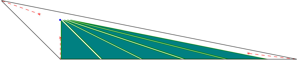 Figure 1
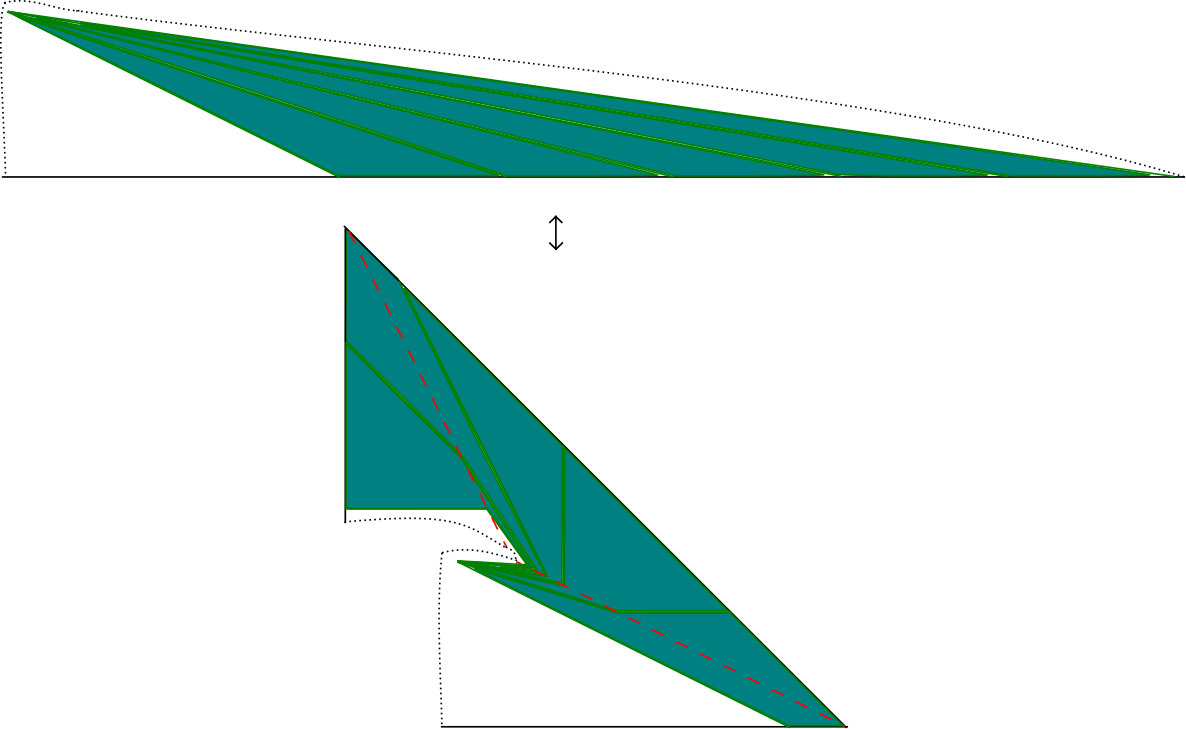 Figure 2
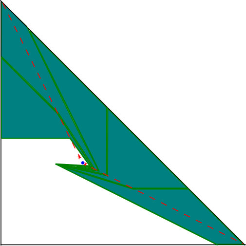 Figure 3
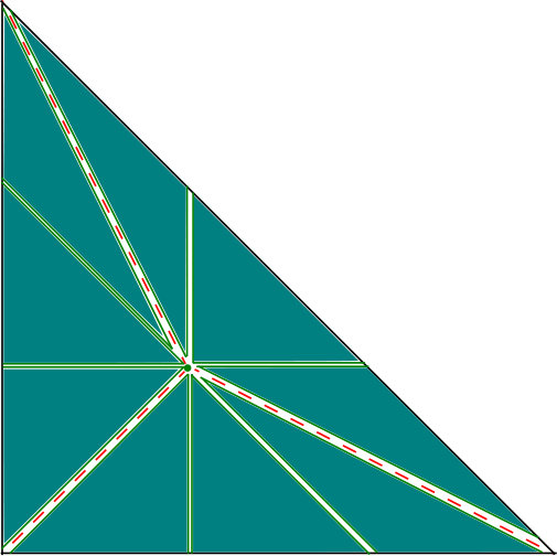 Figure 4
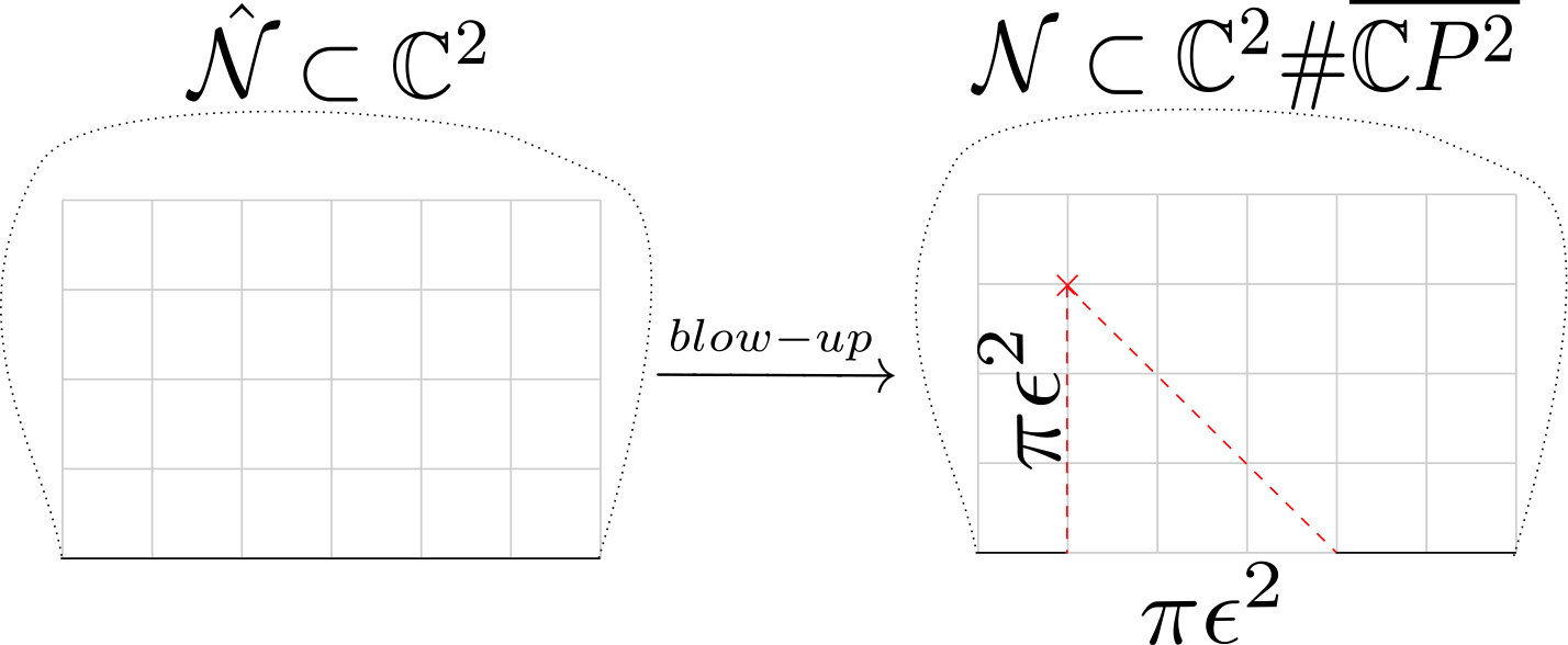 Figure 5
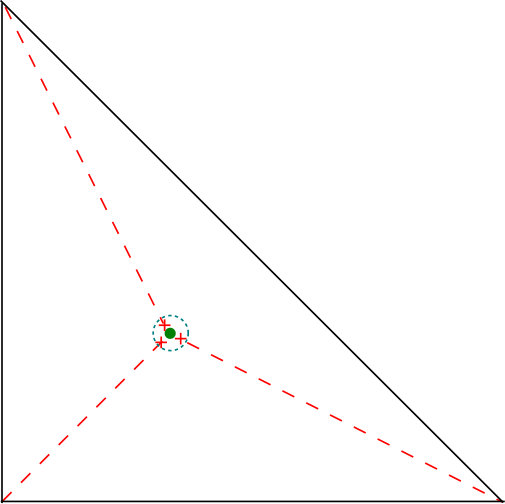 Figure 6
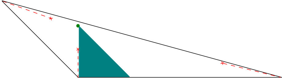 Figure 7
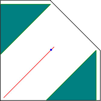 Figure 8
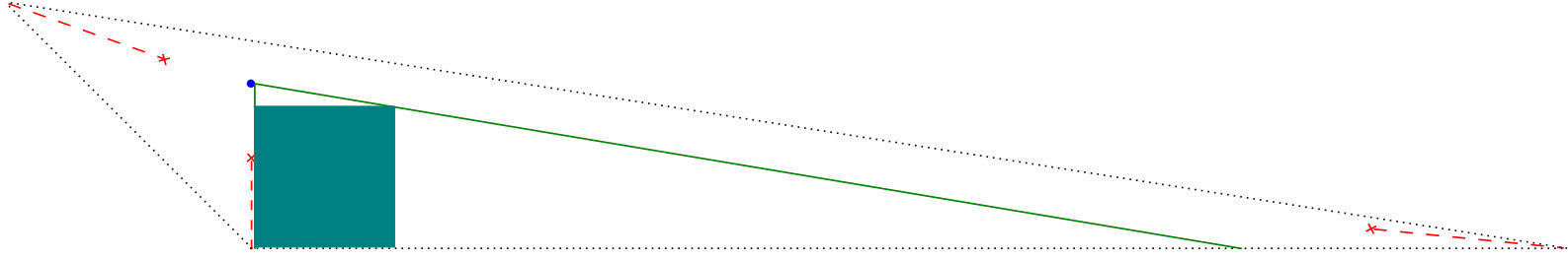 Figure 9
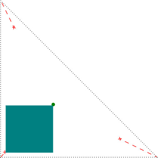 Figure 10
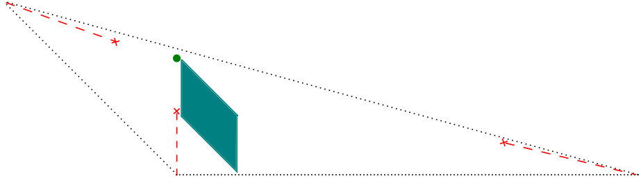 Figure 11
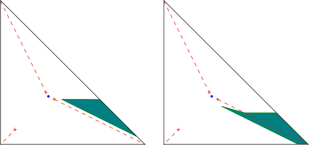 Figure 12
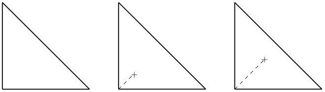 Figure 1
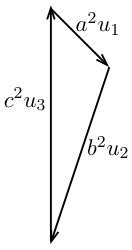 Figure 2
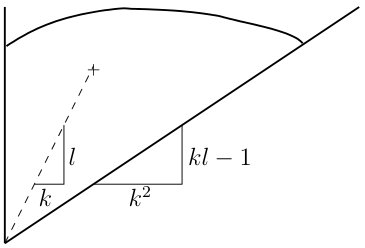 Figure 3
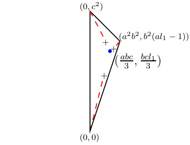 Figure 4
 Figure 17
Peer Reviews
No public reviews on file for this paper yet. If you reviewed it on a platform where reviews are public (OpenReview, ICLR, NeurIPS, ICML), you can paste yours below so the community can read it here.
Videos
No videos yet. Explain this paper in a talk, walkthrough, or lecture? Add one.
Taxonomy
TopicsGeometric and Algebraic Topology · Geometry and complex manifolds · Geometric Analysis and Curvature Flows
Asymptotic behavior of exotic Lagrangian tori in as
Weonmo Lee, Yong-Geun Oh, Renato Vianna
Weonmo Lee
Department of Mathematics, POSTECH, Pohang, Korea & Center for Geometry and Physics, Institute for Basic Sciences (IBS), Pohang, Korea
Yong-Geun Oh
Center for Geometry and Physics, Institute for Basic Sciences (IBS), Pohang, Korea & Department of Mathematics, POSTECH, Pohang, Korea
Renato Vianna
Institute of Mathematics, Federal University of Rio de Janeiro (UFRJ), Rio de Janeiro, Brazil
Abstract.
In this paper, we study various asymptotic behavior of the infinite family of monotone Lagrangian tori in associated to Markov triples described in [Via2]. We first prove that the Gromov capacity of the complement is greater than or equal to of the area of the complex line for all Markov triple . We then prove that there is a representative of the family whose loci completely miss a metric ball of nonzero size and in particular the loci of the union of the family is not dense in .
Key words and phrases:
Vianna tori, Markov triple, orbifold projective plane, almost toric fibration, relative Gromov capacity, Lagrangian seeds
2010 Mathematics Subject Classification:
Primary 53D05, 53D35
WL and YO were supported by the IBS project IBS-R003-D1. RV was supported by the Brazil’s National Council of scientific and technological development CNPq, via the ‘bolsa de produtividade’ fellowship, and by the Serrapilheira fellowship
Contents
1. Introduction
In [Via1, Via2], the third named author constructed an interesting family of infinitely many monotone Lagrangian tori in by constructing a monotone Lagrangian torus associated to each of the Markov triples , i.e., positive integers satisfying the equation
[TABLE]
For his construction, it was used constructions almost toric fibration, Symington’s nodal surgery operations [Sym2] or the operation of rational blow down of the weighted projective planes to . Denote by any realization of the torus associated to the triple in its Hamiltonian isotopy class in . To show that this family of are not pairwise Hamiltonian isotopic to one another, he used the disc-counting invariants which are known to be well-defined for monotone Lagrangian tori [EP, Oh4].
The starting point of our research in the present article lies in our attempt to understand the tori in terms of the geometry of Fubini-Study metric on . (We refer to Section 8 for more discussion on the related questions.) As a first step towards this goal, we ask the following question
Question 1.1**.**
Let be a fixed family of tori in . What is the geometric behavior of these tori as ? For example, will the tori densely spread out as ?
We denote by the set of Markov triples. We remark that a specific construction of the tori depends on various unspecified parameters. Because of the way how they are constructed, it is not easy to visualize the tori in the Fubini-Study metric of although they are well-defined up to Hamiltonian isotopy on .
Fix any smooth metric on , e.g., take the Fubini-Study metric of .
Question 1.2**.**
Let be any realization of the family of monotone Lagrangian tori in . Consider the following asymptotic quantity
[TABLE]
where is the distance from to . Is ? If so, estimate this .
More intuitively and equivalently, the question asks if for any given point and a positive constant , there exists a Markov triple such that for the given family .
This number is not a priori a symplectic invariant. More precisely if is another realization of these tori, this quantity may vary. Because of this, we consider the following quantity
[TABLE]
where is the relative Gromov area
[TABLE]
Relative Gromov area is a symplectic invariant and has been systematically studied by Biran and Biran-Cornea [Bir1, Bir2, BC] for general pair of symplectic manifold and its Lagrangian submanifold .
Remark 1.3**.**
We warn the readers that this definition of relative Gromov area is not the one used by Biran and Cornea in [BC]. For our purpose in the present paper, we do not need their finer version and so we will just use the same term instead of introducing another different term for the Gromov area of the complement.
The first theorem we prove in the present paper is the following rather optimal lower bound. (See the construction given in Section 4.)
Theorem 1.4**.**
Let be any of monotone Lagrangian tori of [Via2]. Then
[TABLE]
Here we normalize the Fubini-Study form so that the area of the complex line is .
Motivated by the nature of our construction given in Section 4, we conjecture that the equality holds in the above theorem.
On the other hand, this lower bound is certainly not optimal for an individual torus. For example for the case of Clifford torus corresponding to , it is easy to see and Biran-Cornea [BC] proved , and hence
[TABLE]
This leads us to a very interesting open problem
Problem 1.5**.**
Find the precise estimate of as done for the Clifford torus.
The above theorem still does not prevent the loci of the union of the family being dense in , it may happen that there exists a family of symplectic balls of nonzero size associated to Markov triples which are stretched thin and wildly spread around the ambient space without touching the corresponding torus respectively.
Theorem 1.6**.**
There exists a family of tori that misses some closed metric ball of non-zero size in . In fact, the supremum of the Gromov areas of such metric balls is . In particular, the loci of the family is not dense in .
The proof of this theorem will be given in Section 5 using the geometric mutation theorem of the Lagrangian seeds studied in in [STW] and [Ton, PT]. But one only needs to look at Figure 9 to see how it goes.
In the rest of the paper, we will provide various estimates relevant to the ball packing problem in or where is a smooth cubic curve, which corresponds to a Donaldson divisor of . One of the outcomes is the following result
Theorem 1.7**.**
Any tori, in particular the Chekanov torus, can be embedded into the monotone for .
This in particular affirmatively answers to a question posed by Chekanov and Schlenk [CS, Section 7] which asks whether Chekanov torus can be embedded into .
In Section 8, we make further discussion and propose several open questions related to the geometry of the tori .
2. Review of the exotic tori
The third named author [Via1, Via2] constructed a family of infinitely many non-Hamiltonian isotopic monotone Lagrangian tori in as the transfers to of the fibers at the (labeled) barycenter of the moment polytope of the weighted projective plane or its relevant almost toric fibration. He utilized Symington’s symplectic rational blow-down operations [Sym1] on each neighborhood of orbifold points thereof and Moser’s deformation of the glued symplectic forms on the resulting blow-down to the Fubini-Study form on for his construction. For the simplicity of notation, we denote by
[TABLE]
any realization of the family of these tori in their Hamiltonian isotopy class in . We exclusively reserve for the fiber at the barycenter of the moment polytope of . The torus can be also realized as the fiber of a base point of an almost toric fibration of [Via2]. An almost toric fibration is a singular Lagrangian fibration with nodal singular fibers. Here a nodal singular fiber carries an isolated singularity whose image under the almost toric projection lies on the interior of the base diagram of the almost toric fibration. This image point is called a node.
2.1. Almost toric fibration and nodal surgeries
In this subsection, we recall definitions of almost toric fibration, nodal surgery operation and related results from [Via1, Section 2.3].
Definition 2.1** ([Zun1], [Via1]).**
An almost toric fibration of a symplectic four manifold is a Lagrangian fibration such that any point of has a Darboux neighborhood (with symplectic form ) in which the map has one of the following forms:
[TABLE]
with respect to some choice of coordinates near the image point in . An almost toric manifold is a symplectic manifold equipped with an almost toric fibration.
A Lagrangian fibration induces an integral affine structure on the base with singularity. Such pair is called an almost toric base [Sym2]. For an almost toric manifold, there is a nontrivial monodromy around the nodal singular fiber. This prevents one from embedding the full almost toric base into where is a standard integral affine structure. However removing an embedded curve joining a point of the boundary, in particular the vertex, of a moment polytope and the node, called a branch curve, makes this embedding possible.
Definition 2.2**.**
Suppose we have an integral affine embedding , where is an almost toric base and is a set of branch curves. A base diagram of with respect to and is the image of decorated with the following data:
- •
an x marking the location of each node and
- •
dashed lines indicating the portion of that corresponds to .
If the direction of is , then the monodromy around the node can be represented by
[TABLE]
with respect to some choice of basis. (See [Via1] for the details.)
Consider a moment polytope in Nodal trade introduces a node and a cut inside the moment polytope in place of the vertex.(See the first two triangles in Figure 1) The corresponding fibration has a nodal singular fiber and becomes an almost toric fibration. Nodal slide literally “slides” a node along an eigenline of the monodromy map.(See the second and the third triangles in Figure 1)
Following Symington [Sym2], we consider the following operations on almost toric fibrations which do not change the symplectic structure of the total space up to symplectomorphism.
Definition 2.3**.**
Let be two almost toric bases, . We say that and are related by a nodal slide if there is a curve in such that
- •
and are isomorphic,
- •
contains one node of for each and
- •
is contained in the eigenline (line preserved by the monodromy) through that node.
Definition 2.4**.**
Let be two almost toric bases, . We say that and differ by a nodal trade if each contains a curve starting at such that and are isomorphic, and has one less vertex than .
It is shown by Symington [Sym2] that these almost toric operations do not change the diffeomorphism type they represent and keep the symplectic structure up to isotopy and so Moser’s argument shows that the two almost toric manifolds before and after the operations are symplectomorphic.
2.2. as a symplectic reduction of
The base diagram for an almost toric fibration of having a monotone Lagrangian torus at its barycenter looks like the moment polytope of a weighted projective plane , except that the diagram is equipped with nodes and cuts.
In this subsection we describe various aspects of geometry of as a toric orbifold. We consider the following action of on defined by
[TABLE]
for . The weighted projective plane with weights as a complex orbifold is nothing but the quotient of by this action. We denote by its element represented by . is an orbifold with three orbifold points Their corresponding orbifold structure groups are
[TABLE]
respectively.
For our purpose of proving Main Theorem, we need to explicitly express the relevant symplectic structure and -action on starting from the linear sigma model construction as in [Wit, Aud], which was exploited in the Lagrangian Floer theory of toric manifolds in [CO, Section 3]. We regard the toric orbifold as the symplectic reduction of under the action of the circle subgroup for a suitable choice of where is the associated moment map. Then it carries the canonical action of the residual torus thereon. We will call this particular -action the residual -action on .
Now we need to describe this torus action on and its moment polytope explicitly, employing notations from [Abr, Section 2.2]. For this purpose, we start with the standard torus action of on defined by
[TABLE]
This action has its moment map given by
[TABLE]
for an arbitrary choice of constant vector in general where is the basis of dual to the standard basis of . Setting with
[TABLE]
we have
[TABLE]
Being a subgroup, any circle subgroup naturally acts on with moment map
[TABLE]
Then the symplectic quotient of carries the canonical reduced symplectic form and the residual torus action by whose moment map image is the labeled polytope described in subsection 2.3. Furthermore this reduced space is precisely the symplectic orbifold equipped with the 2-torus action by the torus .
We now identify what this circle subgroup associated to is. Define a linear map by
[TABLE]
and denote by the kernel of . We have the short exact sequences
[TABLE]
Denote by the subgroup generated by . also induces the exact sequence of abelian groups
[TABLE]
For any element in , since for all ,
[TABLE]
A simple computation shows
Lemma 2.5**.**
The one-dimensional integral sub-lattice is generated by .
Proof.
Any element in satisfies
[TABLE]
From the second slot,
[TABLE]
This implies
[TABLE]
Here the last equality comes from equalities
[TABLE]
and (2.5) and the fact that is a Markov triple. Therefore is generated by . ∎
Therefore this lemma is consistent with the action (2.1).
2.3. Residual -action on and its moment polytope
Using the generalization of Delzant’s argument applied to toric orbifold, Lerman and Tolman [LT] describe its associated orbifold moment map and the associated symplectic form on explicitly, which we now recall. In order to apply their argument, we borrow relevant definitions and arguments from the exposition of Abreu [Abr, Section 2.2] now.
Definition 2.6**.**
A convex polytope in is said to be simple and rational if
- •
facets meet at each vertex ,
- •
those edges meeting at the vertex are all rational, i.e., each edge has the form where and
- •
the can be chosen to be a basis of the lattice
We call the polytope a labeled polytope if it is a rational simple convex polytope and there is a positive integer label on the interior of each facet.
Theorem 2.7**.**
[LT, Abr]* Let be a compact symplectic toric orbifold, with moment map Then is a labeled polytope. For each facet of , there exists a positive integer , the label of , such that the orbifold structure group of every point in is *
Two compact symplectic toric orbifolds are equivariantly symplectomorphic if and only if their associated labeled polytopes are isomorphic. Moreover, every labeled polytope arises from some compact symplectic toric orbifold.
The following lemma computes the labels of the facets of the moment polytope of , which plays an important role in our proof.
Lemma 2.8**.**
Denote by the moment polytope of of the associated residual -action. Then the label on every facet of is 1.
Proof.
Recall that the orbifold structure group of a point in the weighted projective plane is where is the greatest common divisor of those weights whose component is non-zero. For a point with and , gcd of and is 1. Recall that are mutually coprime. (See [Via2, Proposition 2.2].) Therefore at those points the orbifold structure groups are trivial. Similarly every point but three orbifold points has a trivial orbifold structure group. Therefore each point fibering over the interior of each facets has a trivial orbifold structure group, which means the point is smooth. In other words, the labels of the other facets are 1. This finishes the proof. ∎
Finally we find an explicit coordinate formula of the moment map . Let be the quotient map and the inclusion map. Then by definition of the moment map [MW], the associated moment map satisfies the following equation
[TABLE]
Let (row vector) be the coordinate of and (column vector) be the complex coordinate of . With respect to the standard basis, the map can be written as
[TABLE]
Substituting into the left hand side of (2.2) and setting
[TABLE]
we get
[TABLE]
By equating the first and the last terms of the equation and solving it for , we obtain the coordinate formula of the associated moment map whose value at is given by
[TABLE]
for all . This ends our symplectic description of symplectic orbifold , the -action and its associated moment map .
Remark 2.9**.**
Note that is covered by three orbifold charts. For example, is one of them. This is homeomorphic to where the group action is given by i.e., its associated weights are given by . Denote this orbifold chart as . Similarly, denote and . It is easy to check that on each orbifold chart, the map in (2.3) is invariant under the corresponding group action. Thus is well-defined.
Three orbifold points are mapped to the vertices opposite to the edges associated to , respectively. One can check that points of the form fibers over the points contained in the edge corresponding to . Similarly points of the form fibers over points in the edge , respectively.
We now visualize the image in of the moment map . First we recall that every convex polytope can be written as the intersection of a finite number of oriented half-spaces. To define a labeled polytope, we attach a label on the -th facet and consider the intersection
[TABLE]
where is the -th inward primitive integral vector normal to the -th facet and is areal number.
First we recall the polytope considered in [Via2] for his construction of . In the above expression of general , we consider the edge of affine length , respectively, as the first, second facet. Then we get
[TABLE]
and consider inequalities
[TABLE]
with . We denote the polytope given by this equation by
[TABLE]
This is precisely the one used in [Via2]. See Figure 2.
The following proves that the labeled polytope of the toric orbifold is exactly the moment polytope described above equipped with label 1 on the interior of each facet.
Proposition 2.10**.**
The moment image of given above is (2.4).
Proof.
It is straightforward to check from the explicit formula (2.3). ∎
As described in [Via2], its moment polytope under the residual torus action is the triangle with edges parallel to the vectors where they satisfy the balancing condition
[TABLE]
and have the form
[TABLE]
and with the vertices located at the projection of the orbifold points. From we obtain a relation
[TABLE]
Here each of is a positive integer coprime to respectively. Each of these integers can be realized as a winding number of some section of a trivialization over the boundary of unit disk appearing in the definition of Lagrangian pinwheel, embedded in . (See [Kho, ES].) Furthermore, Evans and Smith [ES] proved that the integers satisfy the following congruence relations;
[TABLE]
Then using the coordinates of , ’s could be computed explicitly from Figure 4 below, and following a series of nodal surgery operations followed by transferring the cut operation, starting from the moment polytope of which corresponds to Markov triple . (See [Via2, Section 2].)
Remark 2.11**.**
When deriving (2.3), using we get another expression for
[TABLE]
Then one can easily check that using coordinates on orbifold charts the image of is exactly . In other words, on , its image point of (2.3) satisfies
[TABLE]
On , the image point satisfies
[TABLE]
On , the image point satisfies
[TABLE]
The associated symplectic form can be written explicitly in terms of labelled polytope data using the analogue of Guillemin’s formula [Gui].
Theorem 2.12**.**
[CDG]* Let be a labelled polytope as above and be the number of facets of . Define a function*
[TABLE]
on . We have
[TABLE]
on .
In our case, and . For in ,
[TABLE]
2.4. Symplectic rational blow-down and almost toric fibration
One realization of the tori is given as the barycentric fibers of various almost toric fibrations on depending on . As mentioned before, its base diagram looks like the moment polytope of except that there is a node at each vertex with a cut in the direction of the corresponding node.
Each small neighborhood of a vertex can be realized as an almost toric base with one node whose boundary is a lens space of the form Let us describe a smooth 4 dimensional manifold fibering on this neighborhood, the corresponding base in and its symplectic rational blow-down surgery.
Let be a pair of coprime positive integers. Consider the base diagram given by the open subset consisting of the points contained in the intersection of the half-spaces
[TABLE]
which is bounded by an arbitrary embedded arc joining two points on the edges respectively contained in the two lines , . It also carries a node on a cut in the direction of the vector .
A smooth 4 dimensional manifold that fibers over is a rational homology ball whose boundary is a lens space This lens space fibers over the embedded arc [Sym2, Section 9.3] contained in .
On the other hand, it is proved in [Via2, Proposition 2.2] that the boundary of a neighborhood of the orbifold point projected to the vertex opposite to is the lens space of the form
[TABLE]
respectively. Here each for is a positive integer coprime to , respectively. Now we consider a small neighborhood of an orbifold point which fibers over the vertex opposite to the edge As two collar neighborhoods of a boundary of and of fiber over the same simply connected base, there exists a symplectomorphism from a collar neighborhood of the boundary of to a collar neighborhood of the boundary of . Similar results hold for the remaining neighborhoods and .(See [Sym1])
Then the rational blow-down surgery replaces a neighborhood of an orbifold point by a rational homology ball , respectively. Furthermore, the symplectic structures and induce a symplectic structure as follows.
As performed in [Via2, Corollary 2.5], applying rational blow-down on each neighborhood of the three orbifold points of yields an almost toric fibration of . We denote by the total space of this almost toric fibration for some base . More precisely, applying the rational blow-down surgery on each neighborhood of three orbifold points in , we obtain an almost toric manifold symplectomorphic to
[TABLE]
equipped with an interpolated symplectic form
[TABLE]
Here each is a cut-off function which is on the corresponding rational homology ball and [math] otherwise. And are suitably chosen positive real-valued functions so that becomes nondegenerate and closed.
Corresponding to base diagram , has three nodes with eigenrays [Via2]) pointing towards
[TABLE]
issued at the vertices opposite to , respectively. The three eigenrays meet at one point, the labeled barycenter, in the interior of . (See Figure 4. Red dashed lines represent respective cuts and the blue dot represents the labeled barycenter.)
Following [Via2, Remark 2.3], we set and as the vectors representing cuts. They satisfy relations
[TABLE]
[TABLE]
[TABLE]
and
[TABLE]
From (2.10), we have . The slope of is then
[TABLE]
By (2.11), the slope of is
[TABLE]
Also from (2.12), the slope of can be written as
[TABLE]
These three expressions of the slope of are indeed the same.
By translation, we may identify the lower left vertex of with the origin in Consequently vertices opposite to edges respectively are located at the points
[TABLE]
Then we derive using (2.5).
We summarize the above discussion into
Lemma 2.13**.**
Let be the polytope associated to the above base diagram . Then the torus is located at the point
[TABLE]
Proof.
Using the slope formula we derived above, we easily check that the three eigenrays are given by
[TABLE]
and that they meet at one point
[TABLE]
∎
2.5. Normalization of the polytope
When we choose ’s and ’s in (2.8), we require the (volume) normalization condition in addition so that
[TABLE]
Such a choice can be always made by suitably choosing the functions , and then Moser’s deformation trick produces a diffeomorphism between the two symplectic forms and
[TABLE]
such that . We fix such a symplectic (actually Kähler) form . (See [Via1] for more detailed explanation.)
To apply the above mentioned Moser’s deformation to the pair of forms and , we need to suitably normalize the size of the polytope so that the cohomology classes should be the same. Since , we know for some positive constant .
We now determine what this is. We first recall that monotonicity constants of all monotone Lagrangian tori in are the same. For example, the Maslov index discs of in have the same symplectic areas independent of .
On the other hand, by the classification theorem from [CO], there exist three obviously seen Maslov index 2 holomorphic discs attached to which are associated to the facets of the polytope . Denote these holomorphic discs by for corresponding to the -th facet of
The following fact is stated in [Via2, Paragraph after Prop. 2.4] without proof. Because this is an important element in our study of the present paper, we give its proof for readers’ convenience.
Proposition 2.14**.**
Consider the polytope described around (2.4). If we scale by dividing by , then the -symplectic areas of Maslov index 2 holomorphic discs attached to are the same as that of . In particular, for all .
Proof.
We start with the following area formula for holomorphic disc of Maslov index 2 from [CO] for general toric manifolds.
Lemma 2.15** (Theorem 8.1 [CO]).**
Let be the toric symplectic form, which is the reduced form of the standard symplectic form on under the linear sigma model construction. Consider the residual action on and its moment map . Let be the fiber torus based at . Then the symplectic area of the holomorphic disc corresponding to the i-th facet is given by
Using this area formula, we compute
[TABLE]
By (2.5), we compute
[TABLE]
Similarly, for the second facet,
[TABLE]
For the third facet,
[TABLE]
(This explanation shows that every holomorphic disc has the same area as it should be because because Lagrangian tori are monotone.) Therefore after if we scale the symplectic form by , all holomorphic discs of Maslov index 2 has area which is the same as that of Clifford torus of in with respect to . Obviously this area is independent of the choice of Markov triple . ∎
3. Lower bound for the relative Gromov area
Let be a symplectic manifold. We recall the definition of Gromov area. Denote
[TABLE]
for .
Definition 3.1** (Relative Gromov area).**
Let be a compact subset. Consider a symplectic embedding . The relative Gromov area is defined by
[TABLE]
We are interested in studying the behavior as . For this purpose, we first recall two methods of finding a symplectic balls in the context of toric manifolds.
The first one is given by Karshon [Kar] who uses the shape of triangle and the other is given by Mandini and Pabiniak [MP] who uses the shape of diamond in the moment polytope.
3.1. Almost toric blowup and symplectic balls
In this subsection, we follow the exposition given in [Via3, Section 2.4] on the almost toric blowup to which the readers are referred for details. See also [Zun2, Sym2, LS].
In short, the picture below describes an almost toric blowup. The exceptional curve lies over the dashed line, consisting of one circle on each fibre that collapses as it approaches the edge and as it approaches the node.
In particular, one must be able to find a symplectic ball of Gromov area , in a neighbourhood of an affine triangle in an ATF (almost toric fibration), corresponding to the missing triangle after the almost toric blowup.
More precisely, suppose we see a triangle inside a toric region of an ATF, as illustrated in Figure 6. Viewing the preimage of any small neighborhood of this triangle as a blowdown of the corresponding neighborhood of the exceptional curve as in Figure 5, we can then infer that there is a symplectic ball of capacity projecting into the preimage of this neighborhood of the triangle.
So for our purpose, every time we encounter a triangle as in Figure 6, we know there is a symplectic ball of any given capacity smaller than that projects into the shaded triangle.
Just for visualization purpose, we describe how a symplectic ball centred at a point lying over an edge of an ATF, and projecting into the triangle of Figure 6, should look like.
We first describe how its boundary intersect each fibre of the triangle. To ensure that the topological sphere described below is indeed the boundary of a symplectic four ball, one needs to make more specific choices for these intersections. We omit these details, since by the previous discussion, we do not really need them.
The boundary intersects the corresponding triangle in the toric sector of the ATF as follows:
- a)
Consider the edge of the triangle corresponding to the intersection with edge of the ATF. The circle fibres, corresponding to the relative interior of the edge, intersect in two points. The circles fibering over the endpoints of the edges, intersect in one point each. Hence, intersects the fibre over the edge in a circle. 2. b)
The tori living over the remaining edges of the triangle intersect in one circle. The class of this circle is the collapsing class associated to the edge. So the circles collapse to a point as we approach the edge, which is consistent with the previous item a). 3. c)
The tori living over the interior edge, intersect in two circles, also in the collapsing class associated to the edge. Hence, they collapse to two points as we approach the edge of the item a). If we approach the fibres of described in item b), these two circles collapse to the corresponding single circle.
In particular, consider a segment in the triangle, parallel to the edge of the ATF, connecting points of the edge of the triangle. It divides the triangle in two parts, the top part being a similar triangle. The intersection of with the fibres over this segment form a torus. The top part then intersects in a solid torus, where the family of tori living over the corresponding parallel edges collapse to the circle living over the vertex. The bottom part also intersects in a solid torus, now the corresponding parallel segments converge to the edge of the intersecting the edge of the ATF, whose fibres intersect in a circle, as in item a) above. It is easy to see that this circles correspond to generators of of the torus living over our initial segment. Hence, we have indeed .
To get , we consider ’s as above, projecting to smaller triangles similar to each other, eventually collapsing to a point in the middle of the edge of the starting triangle.
One is able to see that we can get balls of any capacity smaller than , projecting inside our given triangle. In particular, we can get a symplectic ball of capacity , if we get this triangle inside a slightly bigger one in our ATF.
3.2. Method by Mandini and Pabiniak [MP]
We first recall a result by Mandini and Pabiniak [MP]. Following [MP], we consider the subset
[TABLE]
Proposition 3.2**.**
[MP]* For each the 4-ball of capacity symplectically embeds into . Therefore, if for a toric manifold with moment map ,*
[TABLE]
for some and , then the Gromov area of is at least .
Construction of such a symplectic embedding of a 4-ball into is given in the proof of [LMS, Lemma 4.1] using [Sch, Lemma 3.1.8] which is irrelevant to the toric structure of a symplectic manifold. They use only an area-preserving map from a 2-ball of capacity to rectangle , sending concentric circles to loops, rectangles with four corners smoothed such that the area enclosed by each smoothed rectangle in is equal to the area enclosed by a concentric circle in the 2-ball, in .
Let be a toric symplectic manifold. If an affine transformation maps a diamond into the interior of then some subset of is symplectomorphic to Here we use the identification Then the above symplectic embedding of the diamond induces a symplectic embedding of into
Adopting the same idea in the almost toric case, not only for toric manifolds but also for almost toric manifolds, Proposition 3.2 will hold the case with suitable modifications.
Proposition 3.3**.**
Let be an almost toric manifold with almost toric fibration If for some and , then the Gromov area of is at least
Proof.
A crucial ingredient in the toric case exploits the fact that each fiber over an interior point of its moment polytope is a 2-torus and we have symplectically via the action-angle variables. Let be an almost toric fibration. In the almost toric base a smooth fiber over its interior point is a 2-torus away from the singular values of .
Assume that there is an affine transformation of mapping into Then some subset of is symplectomorphic to Symplectic embedding of the 4-ball of capacity into in [LMS] completes the proof. ∎
Remark 3.4**.**
Recall that both nodal trade and nodal slide operations induce two diffeomorphic smooth 4-manifolds with isotopic symplectic forms. Performing nodal slide of a node towards either the vertex or the barycenter of a base diagram along each eigenray allow us to find the size “” of a diamond while avoiding all nodes inside the base diagram. Since Gromov area is invariant under a symplectomorphism, combining these, we can find a maximal lower bound for the Gromov area of an almost toric manifold.
4. Symplectic balls in the complement of in .
By the discussion given in Subsection 3.1, in order to see a symplectic ball in the complement of , it is enough to identify a corresponding triangle with one side in the edge of the ATF base diagram, or a diamond in the interior of the base avoiding .
For the simplicity of the constants appearing in this section, we scale the symplectic form so that the area of the Maslov index 2 disk is or the area of the line is . Therefore, each side of the toric diagram has length 3, corresponding to the area of the line and the area of the anti-canonical divisor is 9, since it has degree 3. Therefore, the total area of the boundary of any ATF base diagram is 9. Moreover looking at the orbifold limit the largest edge has length .
We call a monotone triangle, a triangle with one edge at the boundary of the base diagram of the ATF, with all the affine lengths of the edges being , and the associated symplectic ball a monotone ball. Inside a neighbourhood of this triangle projects a ball of capacity one that endows the monotone symplectic form in after blown down.
Theorem 4.1**.**
Rescale the standard Fubini-Study form so that the area of the line is so that the Maslov index 2 disk has area . Then
[TABLE]
Proof.
Up to , we can always take the largest edge of ATF base diagram associated to each Markov triple to be horizontal, with one of the cuts intersecting that edge vertical, as illustrated in Figure 7. Hence the monotone fibre is at height 1. Therefore we can find a equilateral right triangle so that one of the vertices thereof is put right at the point. Because the affine length of the horizontal edge is (in particular grater than 1), we can always find a neighbourhood of a monotone triangle in the complement of the monotone fibre . This finishes the proof. ∎
Even though our construction indicates the lower bound given in the above theorem may be optimal, it is not clear whether it is indeed the case. In fact, as already mentioned in the introduction, the lower bound will be bigger for an individual torus, since we can get a neighbourhood of the monotone triangle – see Figure 7 again. In other words, , for some . As we mentioned in the introduction, Biran-Cornea showed for the Clifford torus in [BC].
However we conjecture the above lower bound is indeed optimal.
Conjecture 4.2**.**
There is no monotone ball in the complement of , and
[TABLE]
with the convention of being the capacity of the monotone ball.
We note that the ball presented in this theorem intersects the ‘boundary divisor’ by construction. Denote by the preimage of the boundary of the base diagram. So we consider , the complement of (still endowed with the finite volume form coming from , i. e., without completing it).
Looking again back at Figure 7, we can indeed see a diamond in the complement of . A small neighbourhood thereof contains a ball of capacity . (See Figure 8.) An application of Proposition 3.3 gives rise to the following initial estimate
[TABLE]
We will give a better improved estimate later in Section after a finer study of the base diagram associated to .
5. Geometry of the locus of the union of
In this section, we construct a representative of the family of monotone Lagrangian tori such that the loci of the tori is not dense in .
5.1. Construction of a non-spreading family }
We consider the configuration formed by the union of the Clifford torus and three Lagrangian disks, as first exposed in [STW], see also [Ton, PT]. We will construct a family such that all tori reside in an arbitrarily small neighbourhood of the locus of this configuration.
We denote for this configuration, which can also be thought as a Lagrangian skeleton of the Liouville domain . This Lagrangian skeleton consists of the monotone Clifford torus together with three Lagrangian disks, with boundaries on .
To make our construction in perspective, we recall the notion of Lagrangian seeds from [PT].
Definition 5.1** (Definition 4.7 [PT]).**
A Lagrangian seed in a symplectic 4-manifold consists of a monotone torus , and a collection of embedded Lagrangian disks with boundary on , which satisfies the following conditions. Here we denote .
- (1)
each is attached to cleanly along its boundary, i.e., transversely in the directions complementary to the tangent lines , 2. (2)
, 3. (3)
, 4. (4)
the curves have minimal pairwise intersections, i.e., there is a diffeomorphism taking each to a geodesic of the flat metric.
With this definition, the above mentioned configuration
[TABLE]
as drawn in Figure 9 is nothing but an example of Lagrangian seed.
The following is the precise statement on which we will be based for this inductive procedure starting from to arbitrarily given .
Lemma 5.2** (Compare with Lemma 4.16 [PT]).**
Denote . Consider the Clifford torus and a Lagrangian disk so that is a mutation configuration. Denote by the Liouville one-form of the exact symplectic form . Then
- (1)
any neighborhood of contains another mutation configuration , 2. (2)
there is an arbitrarily small neighborhood of such that is Liouville, and such that the completion of is isomorphic to the completion of .
The easiest way to see that we can make another mutation configuration as close to the given on as we want is to slide all the nodes of an ATF very close to the monotone fibre – see Figure 9. Say that all the nodes are now inside a small disk in the base. All mutations can then be achieved by sliding the nodes inside , so that the fibration remains unchanged in the complement of . In other words, all the monotone fibre live in the pre-image of – see Figure 9.
We would like to emphasize that this mutation operation is done in a way that the ambient symplectic form, say, the Fubini-Study form unchanged. In particular the union of all these tori is not dense in with respect to the Fubini-Study metric. In fact, our construction shows that the whole family can be put into an open set of arbitrarily small volume by taking the above mentioned neighborhood as small as we want.
5.2. Ball packing in the complement of all these tori
Inside the standard toric diagram of , projects into the barycentre, union the three segments from the barycentre to the vertices, illustrated as dashed lines in Figure 10.
So, as Figure 10 also illustrates, we can find 9 symplectic balls of the same size in the complement of , hence in the complement of all Lagrangian tori, for any capacity smaller than the capacity of the monotone ball.
This is the maximum we can get for volume reasons.
6. Ball packing in the complement of individual torus
We can easily see three monotone balls of the same size in the complement of the Clifford torus in , via the toric blowup.
In [CS, Section 7], Chekanov-Schlenk ask if one can embed the Chekanov torus into the monotone . The answer is yes and we can indeed easily find two extra monotone balls in the complement of the Chekanov torus inside – see Figure 11.
We recall that in an almost toric fibration, we do have the fibres over the cuts, only the affine structure of the base diagram is not corresponding with the standard affine structure of . In particular, we can have a triangular region passing through the cut – see Figure 12. The monodromy may distort the edges of the triangle as it crosses the cut.
This allow us to get even better results for the ball packing. Start with a configuration of 5 consecutive balls, similar to the ones in Figure 10. Consider an ATF with two cuts very close to the monotone Cliford torus. Slide this 5 balls through the cuts as illustrated in Figure 12. You can then “inflate the triangles”, so all of them become monotone triangles. You get a diagram as illustrated in Figure 13.
Of course, when we want to embed the monotone balls, we need a tiny neighbourhood of the monotone triangle. So all these triangles need to be spaced out by a tiny amount, which is not drawn on Figure 13 for visual purposes. Figure 14 illustrates how the balls look like when we undo the monodromies associated with the cuts for better understanding.
These 5 monotone balls are indeed in the complement of tori of the form , all together, in particular of both Clifford and Chekanov tori. This is because all these tori are obtained by changing the ATF in the pre-image of a small region containing the monotone fiber and the two singular fibres – recall the analogous discussion given in Figure 9.
Remark 6.1**.**
We cannot use this trick in the ATF illustrated in Figure 9, to get a monotone ball in the complement of and, hence, of all tori simultaneously. If you try to “slide one triangle of Figure 10 through a cut”, with a triangle of size close to the monotone one, it will be forced to cross all the three cuts several times, in a spiral fashion, before eventually entering the dashed neighbourhood in Figure 9.
To proceed further, we need to make some computations regarding Markov triples ,
[TABLE]
The following is well-known
Lemma 6.2**.**
If the .
Proof.
since . ∎
In particular, if , then and .
Lemma 6.3** (Section 3.7 of [KN]).**
Two out of the three possible mutations of the Markov triple increase the sum and the other reduces it.
(In fact, we can indeed deduce from this that if then , but we won’t need that.)
Proposition 6.4**.**
Suppose . Then
[TABLE]
Proof.
We first transform (6.1) as follows:
[TABLE]
[TABLE]
We will prove, by induction on the biggest Markov number, that if then . This holds for our base .
Suppose that for and consider mutations that increase the biggest Markov number in the triple. We derive from Propositions 6.2 and 6.3 that the mutations that increase the biggest Markov number in the triple are and being the biggest number in the triple and the biggest number in the triple .
So we need to show that
[TABLE]
But we already saw that in the proof of Proposition 6.2:
[TABLE]
[TABLE]
This finishes the proof. ∎
The inequality (6.1) means that, if the affine lengths of the edges are , , , then the longest edge has at least of the sum of the affine lengths .
The sum of lengths of the edges is times the size of the base of the monotone triangle. This means that the longest edge has at least times the length of the base of the monotone triangle. Hence we can see at least 5 monotone balls in the complement of , for , see Figure 15.
Since we have already showed in Figure 13 that we can find 5 monotone balls in the complement of the Clifford torus , we derive that we can find 5 monotone balls in the complement of the union for all .
We summarize the above discussion into the following
Theorem 6.5**.**
Any tori, in particular the Chekanov torus, can be embedded into the monotone for .
This affirmatively answers to a question asked by Chekanov and Schlenk [CS, Section 7]. (See Theorem 1.7 and the discussion around it.)
7. In the complement of an elliptic curve
By [Sym2, Proposition 8.2], we know that the preimage E of the edges of a almost toric fibration diagram, with no rank [math] singularities (i.e., all nodes pushed inside) is a smooth symplectic torus representing the anticanonical divisor. By a result of Sikorav [Sik2, Theorem 3], see also [ST], we can assume that this boundary is indeed an elliptic curve.
In this section we improve the estimate (4.1) further combining the results from the previous section.
From Proposition 6.4, we see that if we can embed, in the complement of in an ATF of , triangles as close as we need to the triangle of height equal to the height of the monotone triangle and base equal 6 times the base of the monotone triangle – see Figure 16.
Inscribed inside one of these triangles we can embed a square of sides with length as close to the height of the monotone triangle as we want, i.e., a diamond – see Figure 16. Hence we can embed a ball of capacity as close to as we want.
Moreover, in the complement of the Clifford torus in we can get diamonds as close to as we want, hence with capacities converging to – see Figure 17.
We summarize the above discussion into the following
Theorem 7.1**.**
[TABLE]
8. Discussion and open questions
In this section, we would like to propose a few interesting open questions in relation to the geometry of in addition to Problem 1.5.
8.1. Hamiltonian-minimal representative
As mentioned in the introduction, the starting point of our research in the present article lies in our attempt to visualize the tori in terms of the geometry of Fubini-Study metric on . One interesting question is to find a geometric realization of the tori with special Riemannian geometric properties in the spirit of [Oh1, Oh2, Oh3].
Question 8.1**.**
- (1)
Construct a Hamiltonian-minimal representative in each Hamiltonian isotopy class of with respect to the Fubini-Study metric and visualize the representative. 2. (2)
More boldly prove that there exists a Hamiltonian-minimal representative of in its Hamiltonian isotopy class, or that there is a lower bound of the volume inside the Hamiltonian isotopy class. 3. (3)
Is there any alternative group theoretic construction of ?
According to [Oh3], the mean curvature flow of Lagrangian submanifolds in Einstein-Kähler manifolds such as in equipped with Fubini-Study metric preserves the Lagrangian property and decreases the volume.
On the other hand, it follows from [Oh2] and the index calculation given by Urbano [Urb] that any Hamiltonian-stable Hamiltonian-minimal Lagrangian torus with respect to the Fubini-Study metric is isometric to the Clifford torus in , provided it is smooth. Therefore none of smooth representative are Hamiltonian-stable unless . This in particular implies that there is no smooth volume minimizing representative of in its Hamiltonian isotopy class unless . It was proven in [Oh2] that the Clifford torus is volume minimizing under a sufficiently small Hamiltonian isotopy, and in particular it is Hamiltonian-stable. These observations reveal that the second question may be a quite hard but interesting question to ask. Existence of a positive lower bound of the volume inside each given Hamiltonian isotopy class can be proved via the Crofton’s formula (see [Oh1, Introduction]), if the following question is affirmative
Question 8.2**.**
Consider the set , i.e., the set of totally geodesic . Is is true that for all . Here denotes the isometry group of the Fubini-Study metric.
Since , the above mentioned non-intersection result follows from the Floer theoretic question whether or not for all . It turns out that this intersection result depends on the types of Markov triples . For example, Alston-Amorim [AA] proved that the Clifford torus intersects for all : They proved that a version of Floer cohomology between the product and in is defined and is non-zero even though the Floer cohomology between and is not defined.
On the other hand, the case i.e., was studied by Wei-Wei Wu [Wu] for which the fiber at the singular vertex of the moment polytope is symplectomorphic to and so it does not intersect the semi-toric fiber . (It is also shown in [OU] that is the Chekanov torus.) In fact, such a non-intersection result can be proved for any triple one of whose element is . This can be seen by mutating the smooth vertices in Wu’s semi-toric picture [Wu], for instance.
These observations lead us to proposing the following conjecture which is an interesting subject of future investigation.
Conjecture 8.3**.**
There exists a Hamiltonian diffeomorphism on such that if and only if .
Finally, under the assumption that the answer to the second question above is affirmative, the following question is interesting to ask.
Question 8.4**.**
Is there a family such that there exists a positive constant
[TABLE]
8.2. Size of Weinstein neighborhood of
Another question is related to the size of the maximal Darboux-Weinstein neighborhood of . We start with some general discussion on Darboux-Weinstein chart. Let be a compact Lagrangian submanifold. Consider the Darboux-Weinstein chart where is a neighborhood of in and is a neighborhood of the zero section . Then by definition, we have
[TABLE]
for the Liouville one-form on and under the identification of with .
Fix any Riemannian metric on . For , we define
[TABLE]
where and is the canonical projection, and is the norm on induced by the inner product .
Definition 8.5**.**
Let be a compact Lagrangian submanifold equipped with a metric . Consider the Darboux-Weinstein chart Define
[TABLE]
and
[TABLE]
over all Darboux-Weinstein chart of . We call the Weinstein width of (relative to the metric ).
The is another symplectic invariant of which measures extrinsic complexity of the embedding . Obviously since for any Darboux-Weinstein chart for compact Lagrangian submanifold .
With this preparation, we propose the following conjecture which is another way of examining the conjectural ergodic behavior of the family .
Conjecture 8.6**.**
Consider . Then
[TABLE]
Proving this conjecture is essentially equivalent to proving the infimum over of the size of the shape invariant is zero. See [Sik1] for the definition of the shape invariant and [STV, Section 6] for the relevant study of this shape invariants.
The reference list from the paper itself. Each links out to its DOI / PubMed record.
- 1[AA] G. Alston and L. Amorim. Floer cohomology of torus fibers and real Lagrangians in Fano toric manifolds. Internat. Math. Res. Notices , (12):2751–2793, 2012.
- 2[Abr] M. Abreu. Kähler metrics on toric orbifolds. J. Differential Geom. , 58(1):151–187, 2001.
- 3[Aud] M. Audin. The topology of torus actions on symplectic manifolds , volume 93 of Progress in Mathematics . Birkhäuser Verlag, Basel, 1991. Translated from the French by the author.
- 4[BC] P. Biran and O. Cornea. Rigidity and uniruling for Lagrangian submanifolds. Geom. Topol. , 13:2881–2989, 2009.
- 5[Bir 1] P. Biran. Lagrangian barriers and symplectic embeddings. Geom. Funct. Anal. , 11(3):407–464, 2001.
- 6[Bir 2] P. Biran. Lagrangian non-intersections. Geom. Funct. Anal. , 16(2):279–326, 2006.
- 7[CDG] D. M. J. Calderbank, L. David, and P. Gauduchon. The Guillemin formula and Kähler metrics on toric symplectic manifolds. J. Symplectic Geom. , 1(4):767–784, 2003.
- 8[CO] C.-H. Cho and Y.-G. Oh. Floer cohomology and disc instantons of Lagrangian torus fibers in Fano toric manifolds. Asian J. Math. , 10(4):773–814, 2006.