Poisson PCA: Poisson Measurement Error corrected PCA, with Application to Microbiome Data
Toby Kenney, Tianshu Huang, Hong Gu

TL;DR
This paper introduces Poisson PCA, a semiparametric method for principal component analysis of Poisson-distributed data, effectively correcting bias and accounting for sequencing depth, with applications to microbiome data.
Contribution
We develop a novel semiparametric Poisson PCA approach that corrects bias in variance estimation and computes principal scores without relying on parametric models.
Findings
Our method outperforms PLN in identifying main principal components.
It is faster and more robust to outliers than existing parametric approaches.
Applications to microbiome data demonstrate practical effectiveness.
Abstract
In this paper, we study the problem of computing a Principal Component Analysis of data affected by Poisson noise. We assume samples are drawn from independent Poisson distributions. We want to estimate principle components of a fixed transformation of the latent Poisson means. Our motivating example is microbiome data, though the methods apply to many other situations. We develop a semiparametric approach to correct the bias of variance estimators, both for untransformed and transformed (with particular attention to log-transformation) Poisson means. Furthermore, we incorporate methods for correcting different exposure or sequencing depth in the data. In addition to identifying the principal components, we also address the non-trivial problem of computing the principal scores in this semiparametric framework. Most previous approaches tend to take a more parametric line. For example the…
Click any figure to enlarge with its caption.
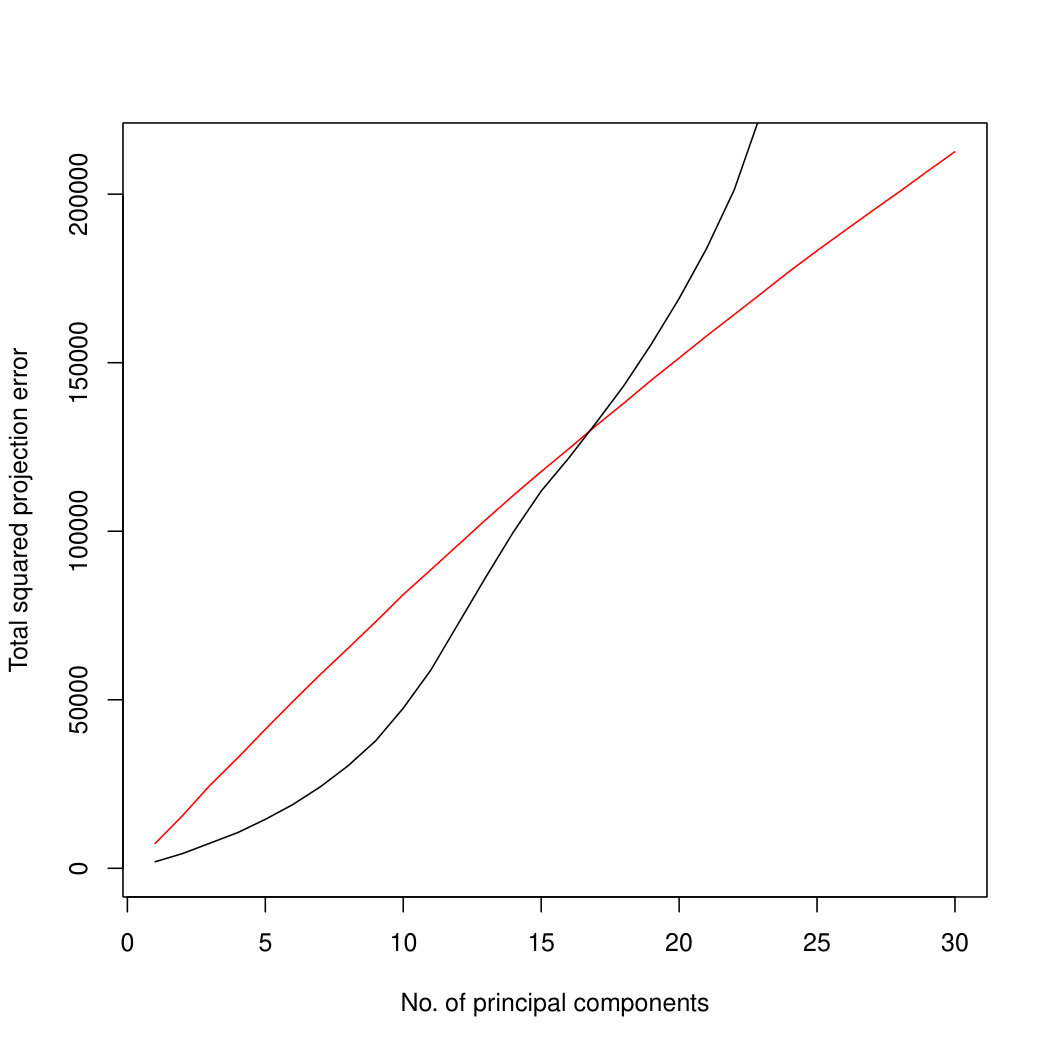 Figure 1
 Figure 2
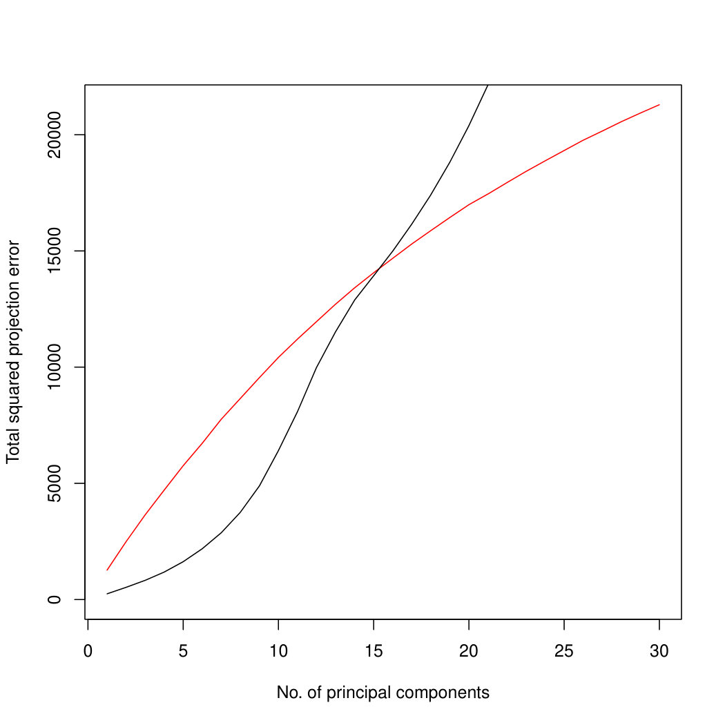 Figure 3
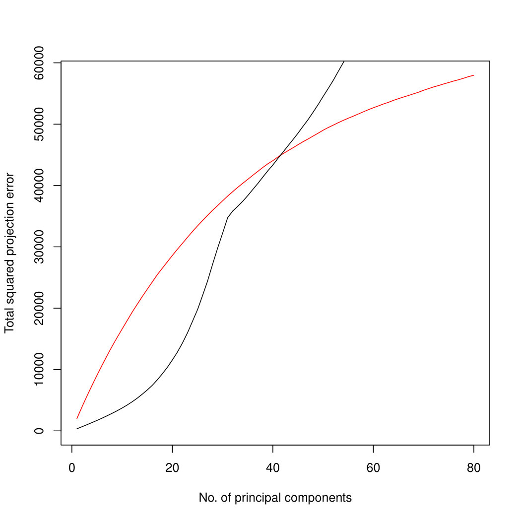 Figure 4
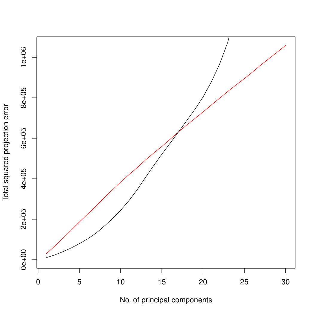 Figure 5
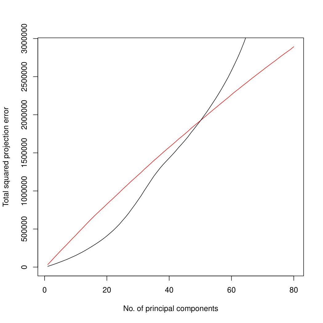 Figure 6
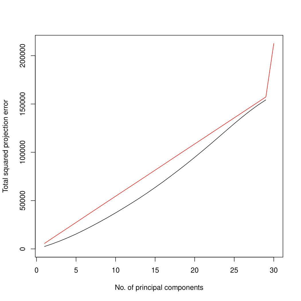 Figure 7
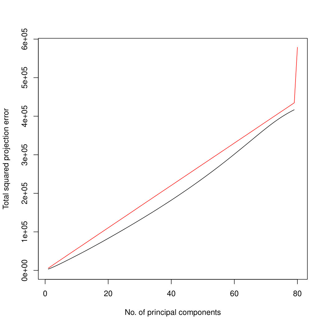 Figure 8
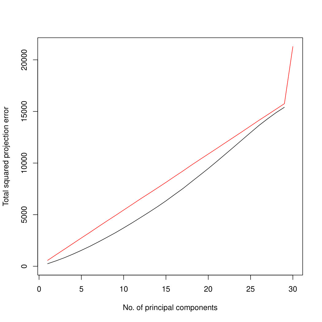 Figure 9
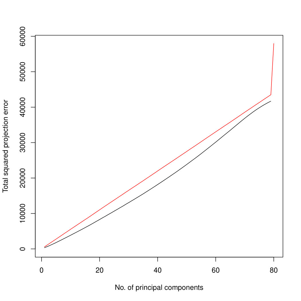 Figure 10
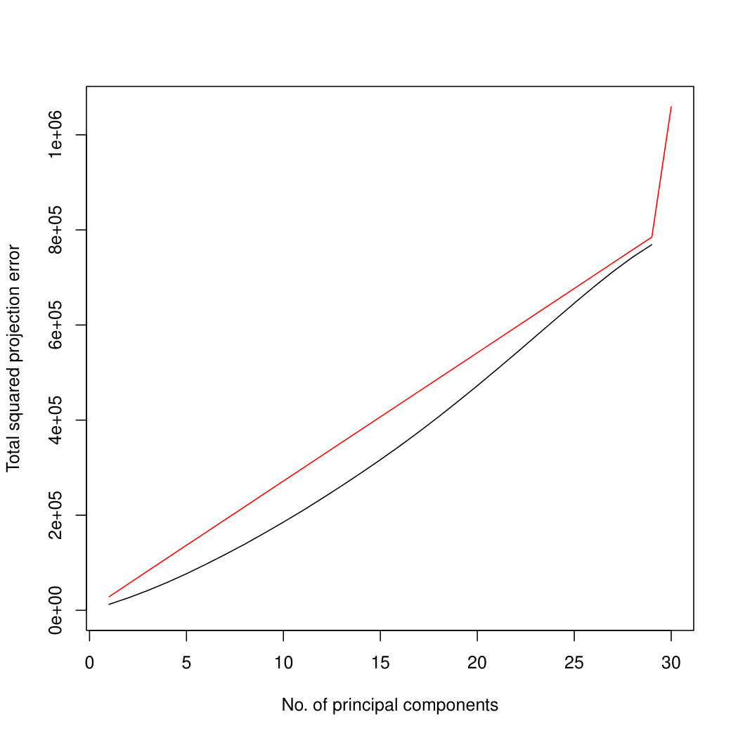 Figure 11
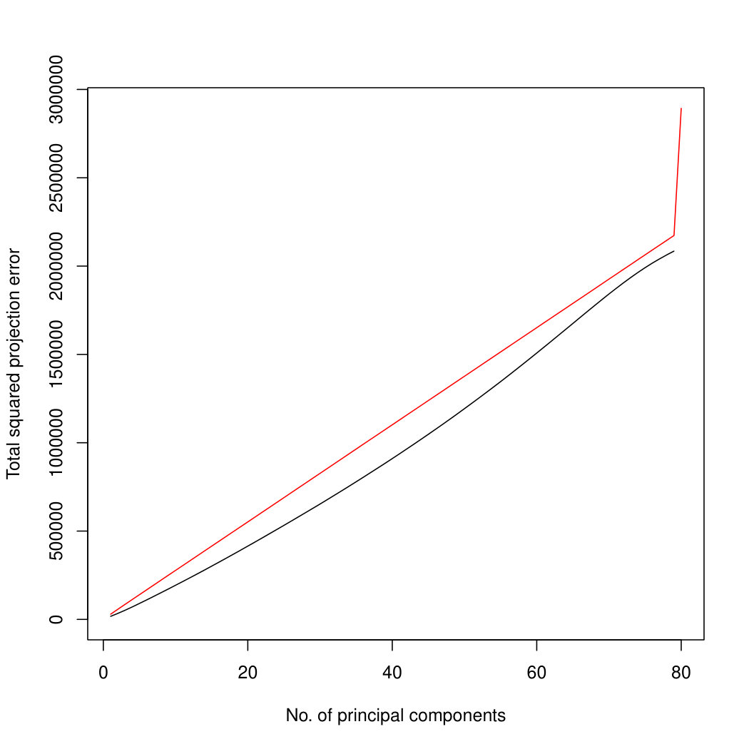 Figure 12
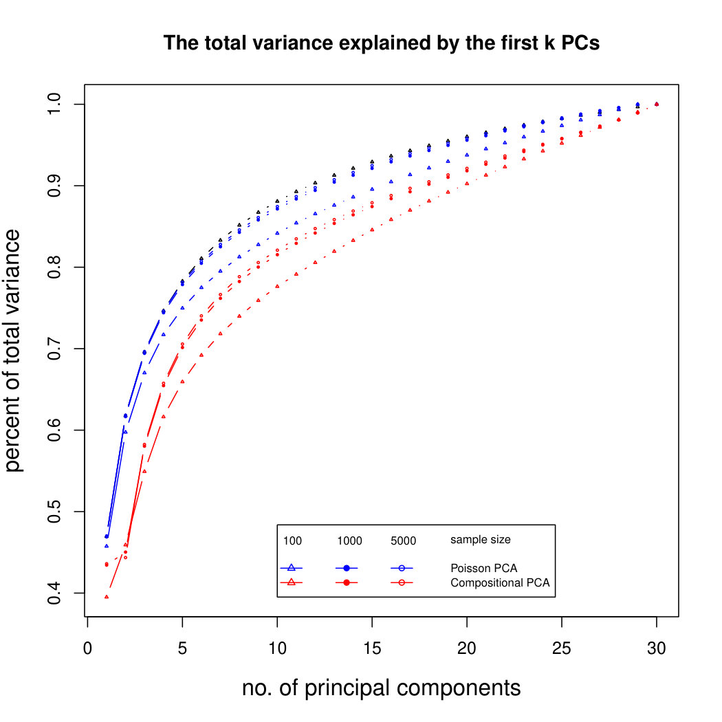 Figure 13
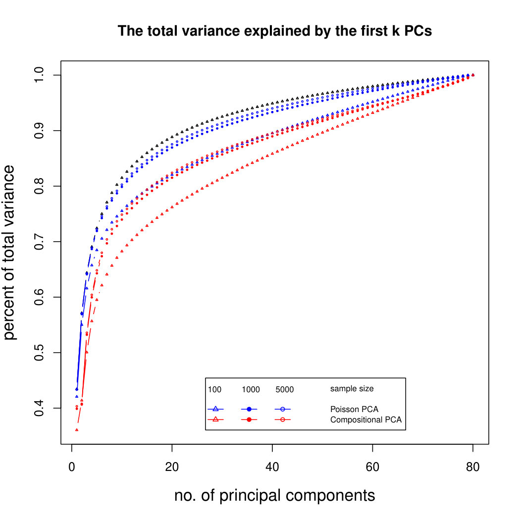 Figure 14
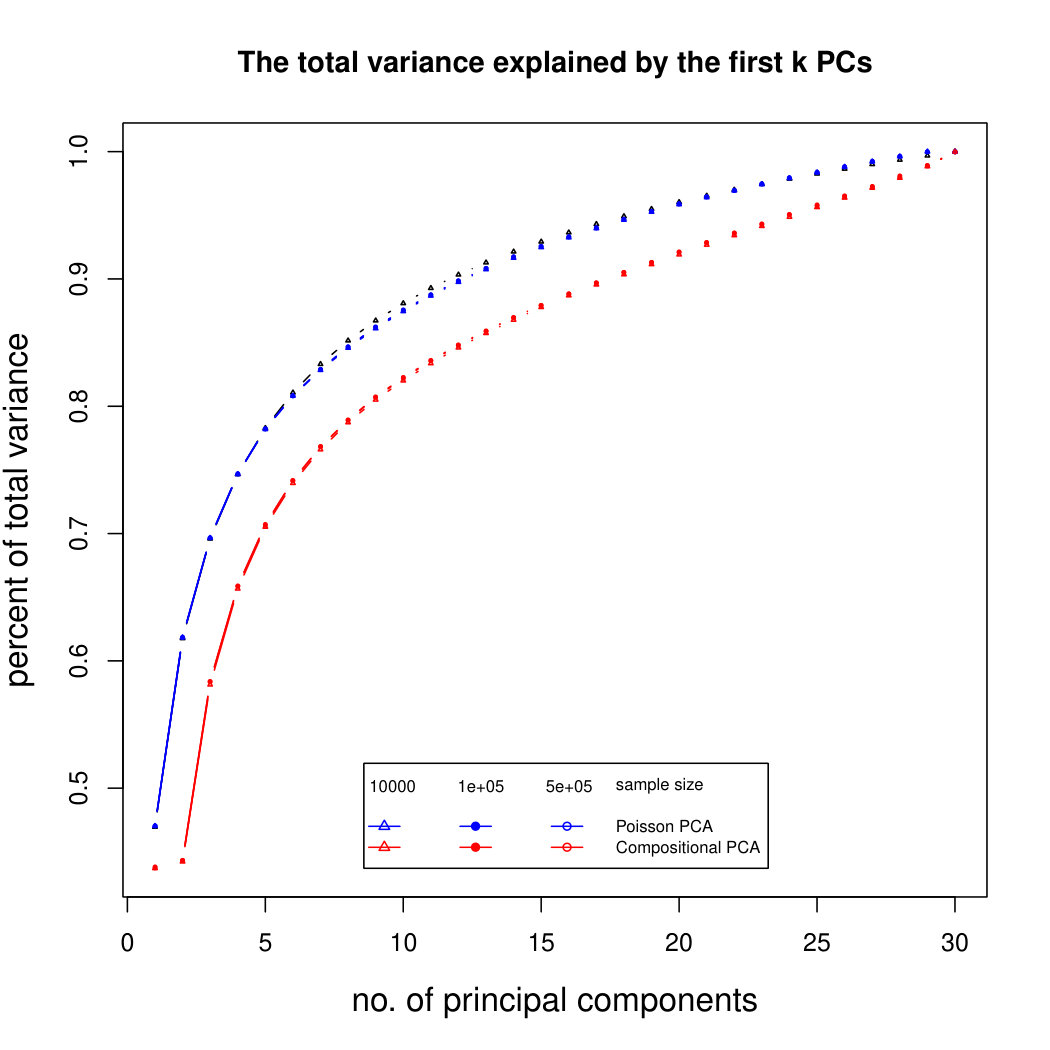 Figure 15
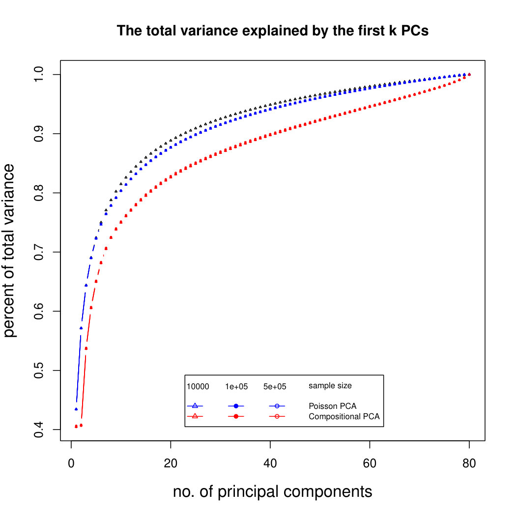 Figure 16
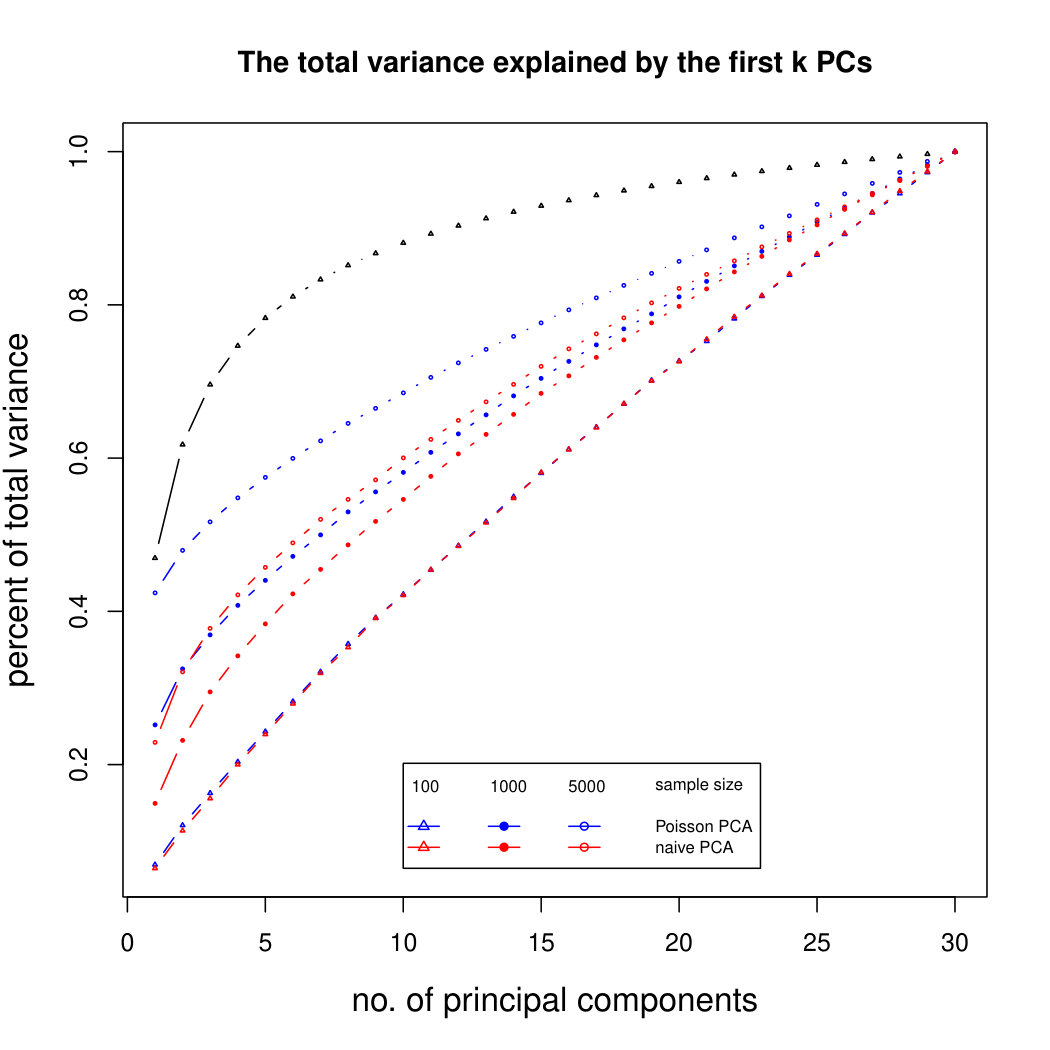 Figure 17
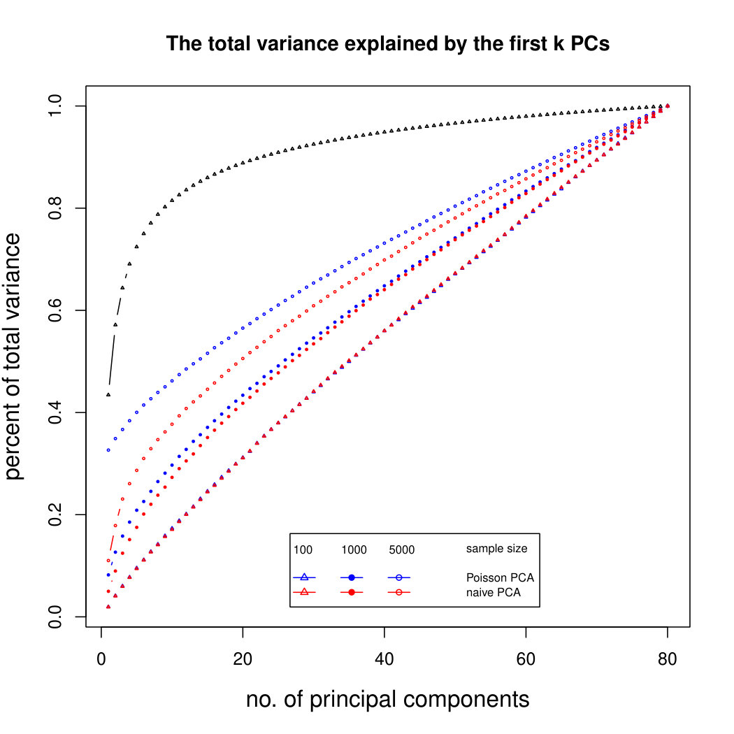 Figure 18
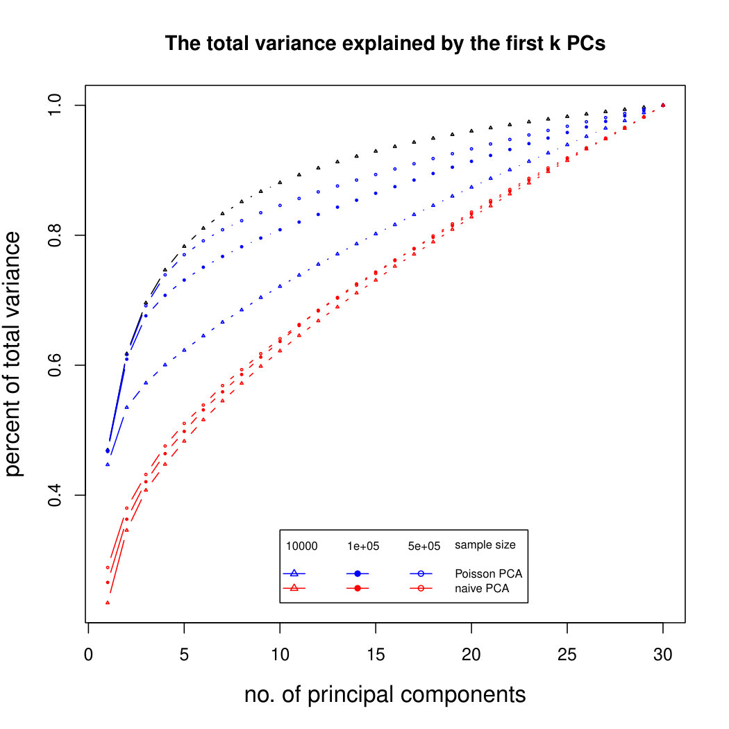 Figure 19
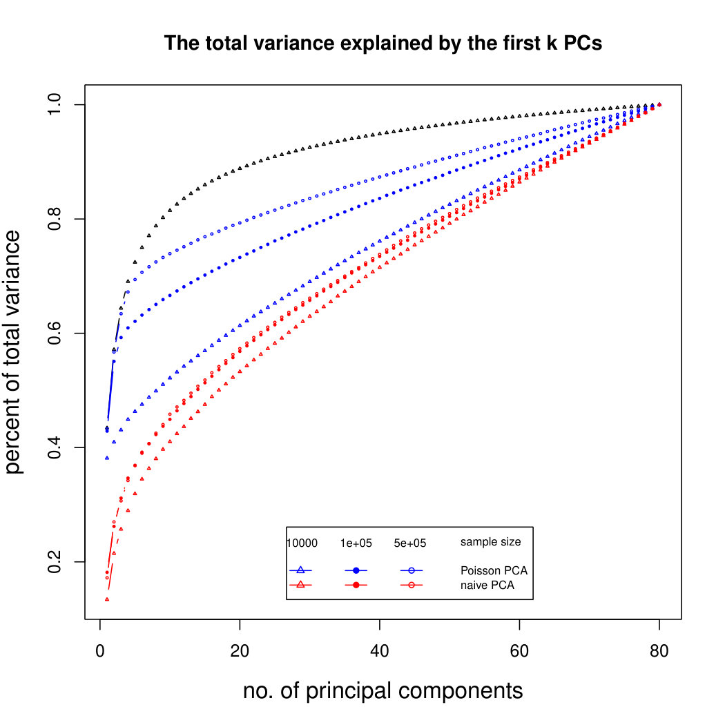 Figure 20
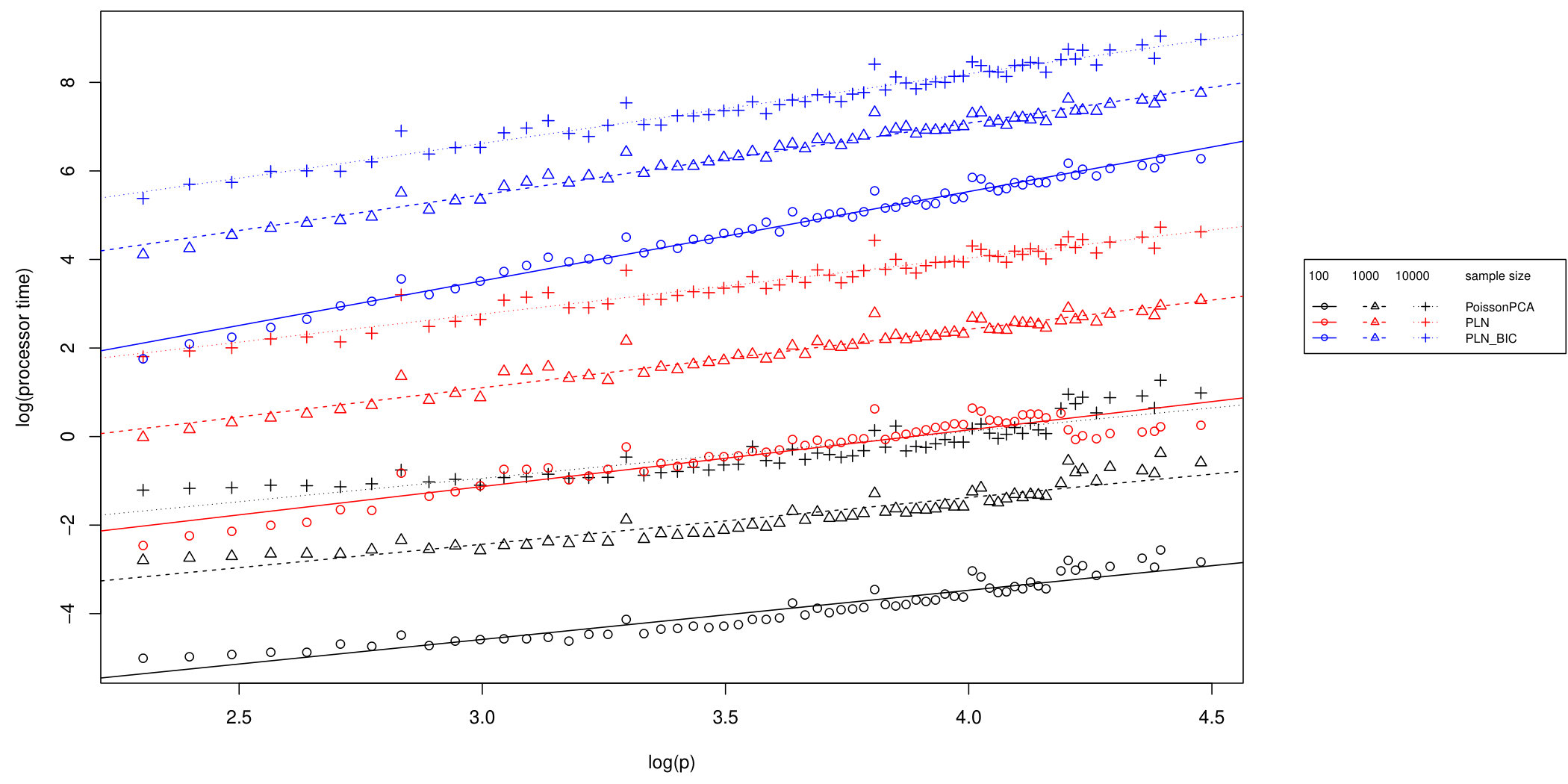 Figure 21
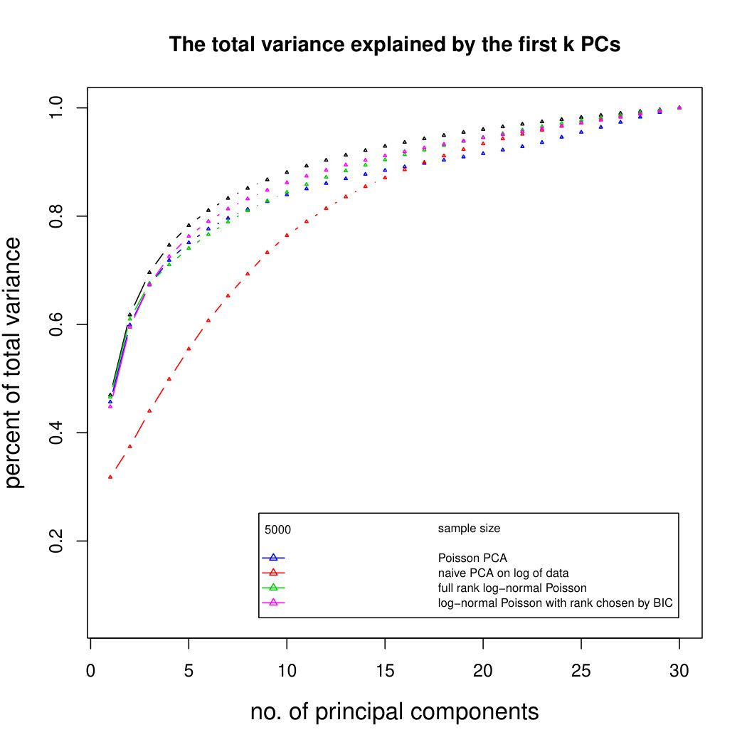 Figure 22
 Figure 23
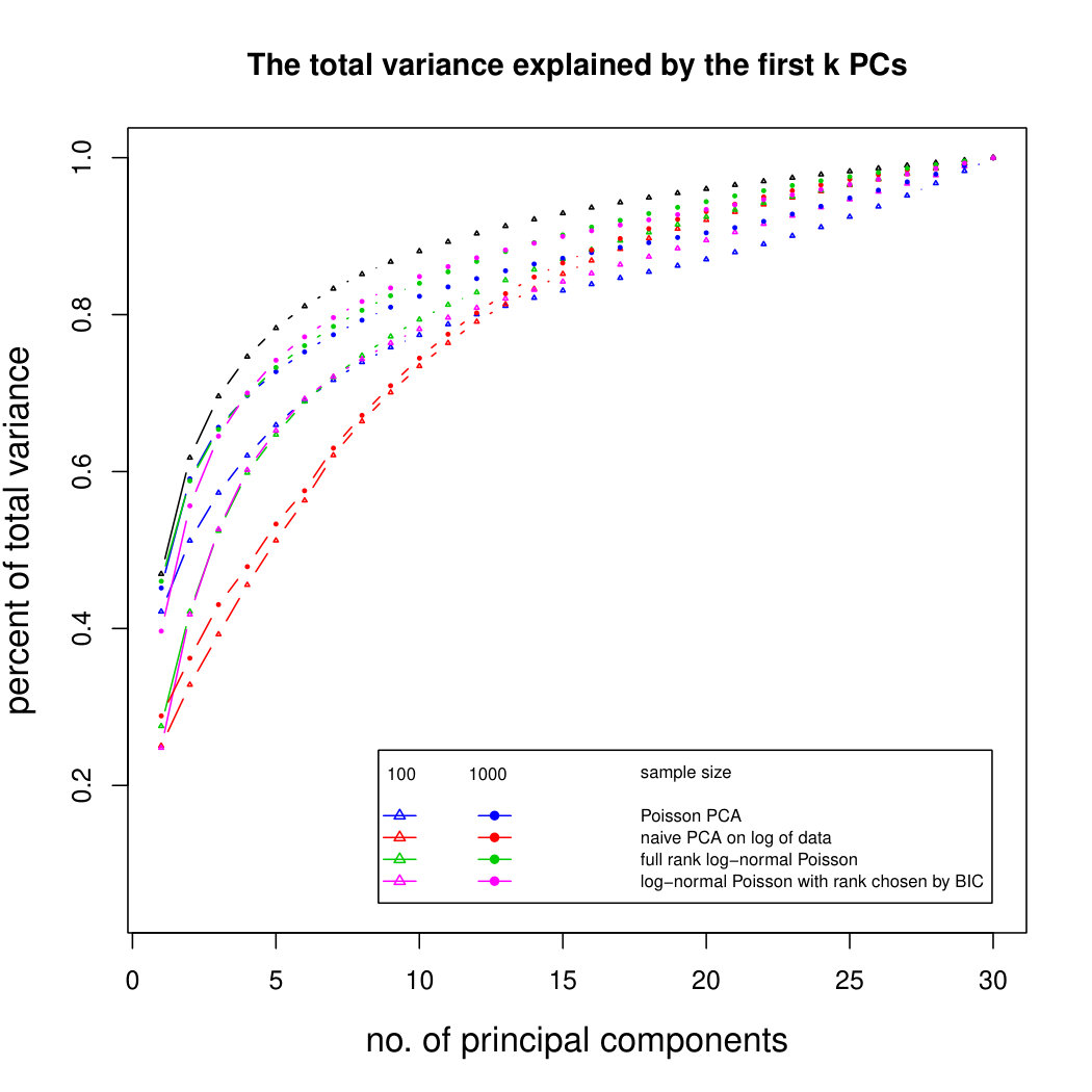 Figure 24
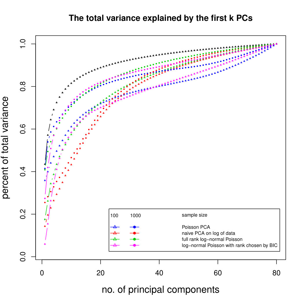 Figure 25
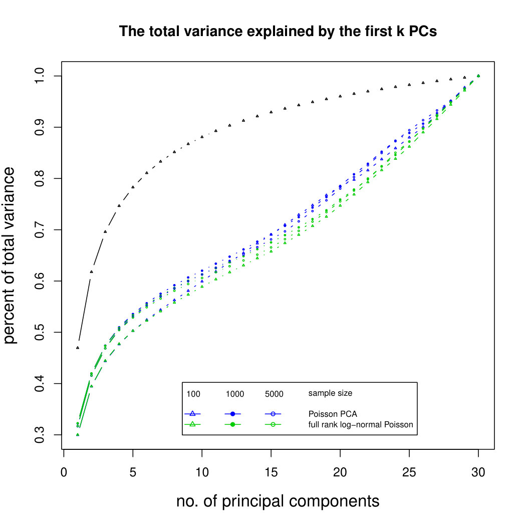 Figure 26
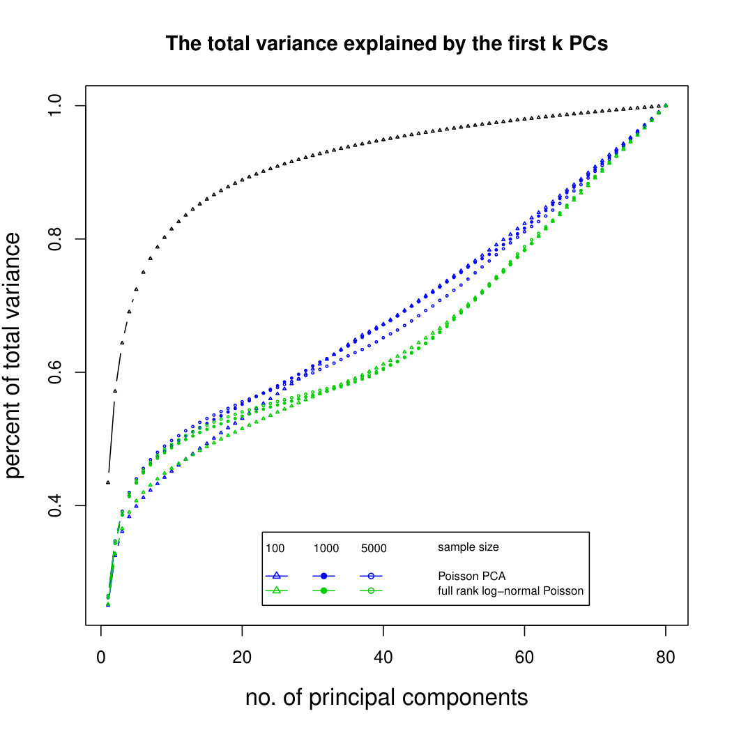 Figure 27
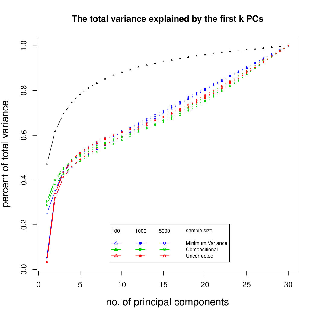 Figure 28
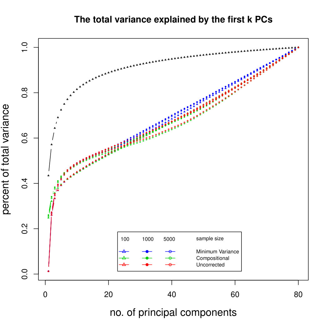 Figure 29
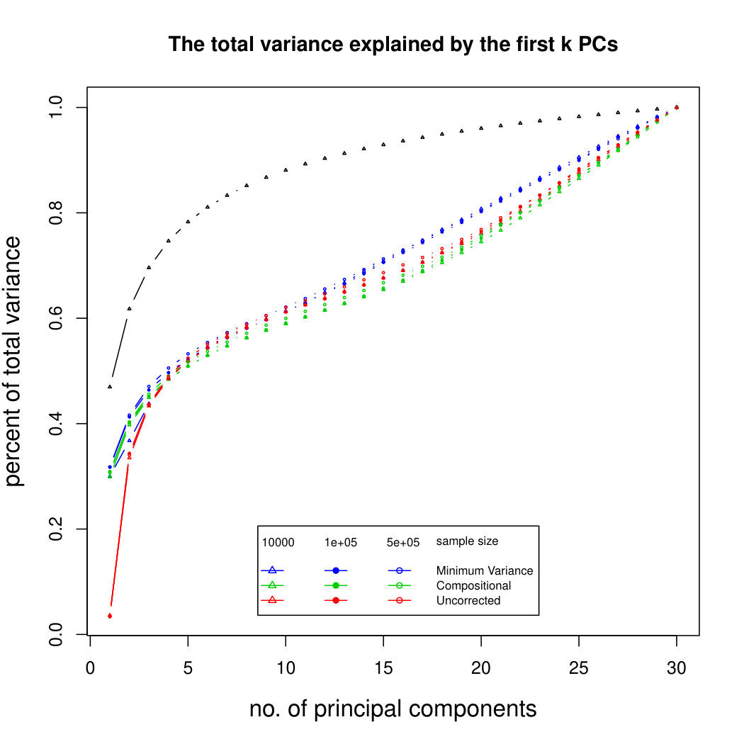 Figure 30
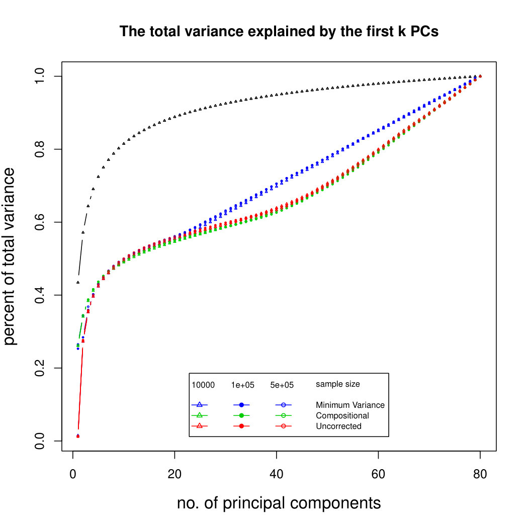 Figure 31
 Figure 32
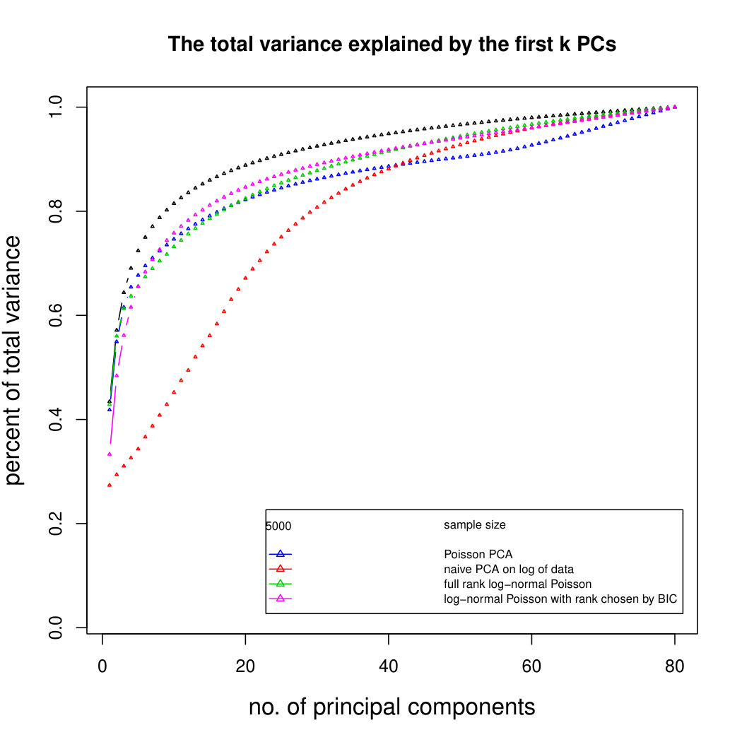 Figure 33
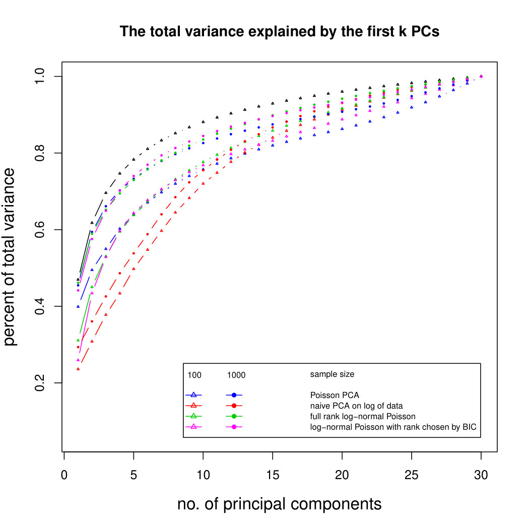 Figure 34
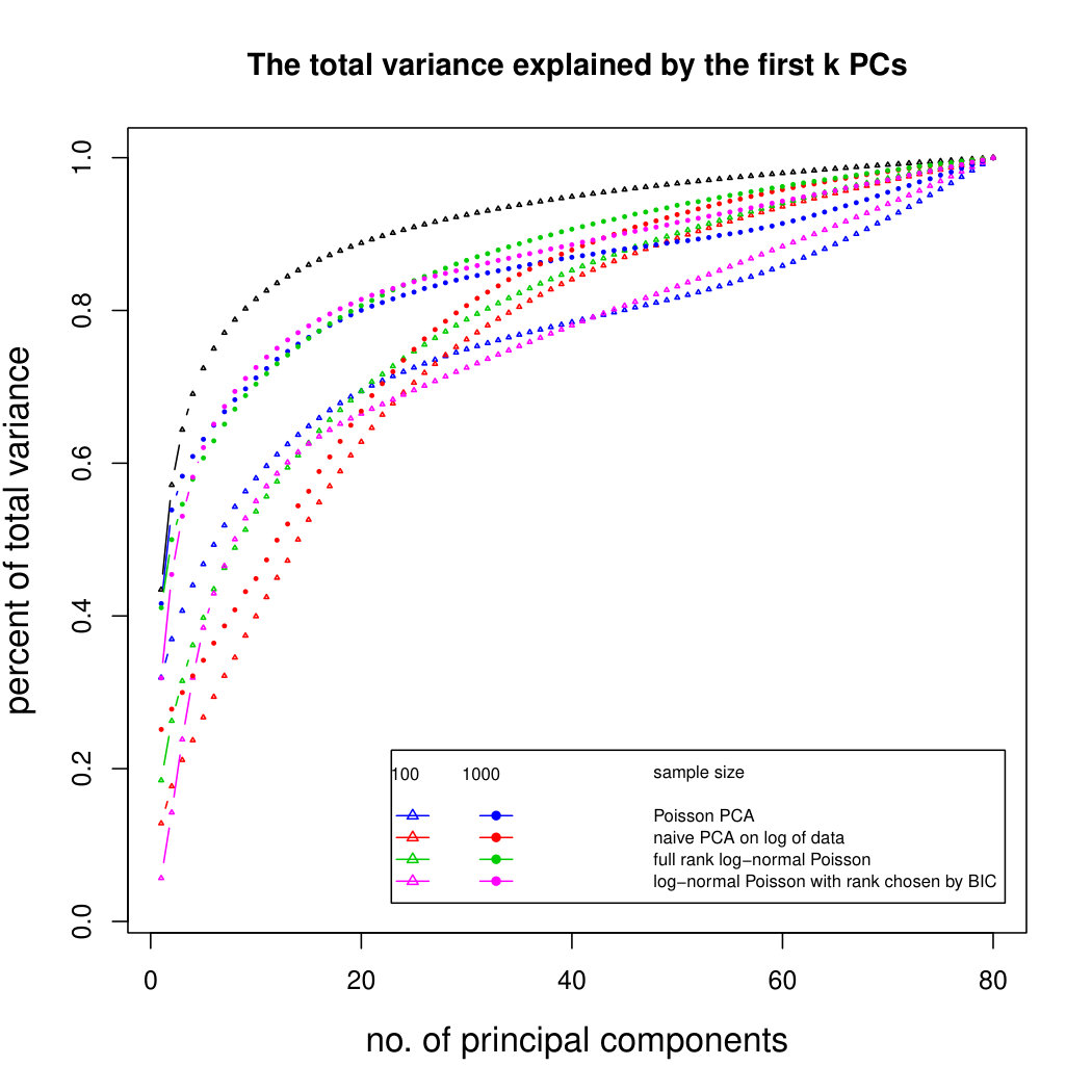 Figure 35
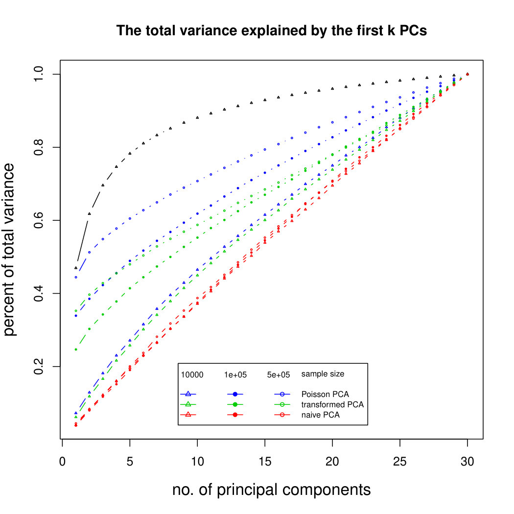 Figure 36
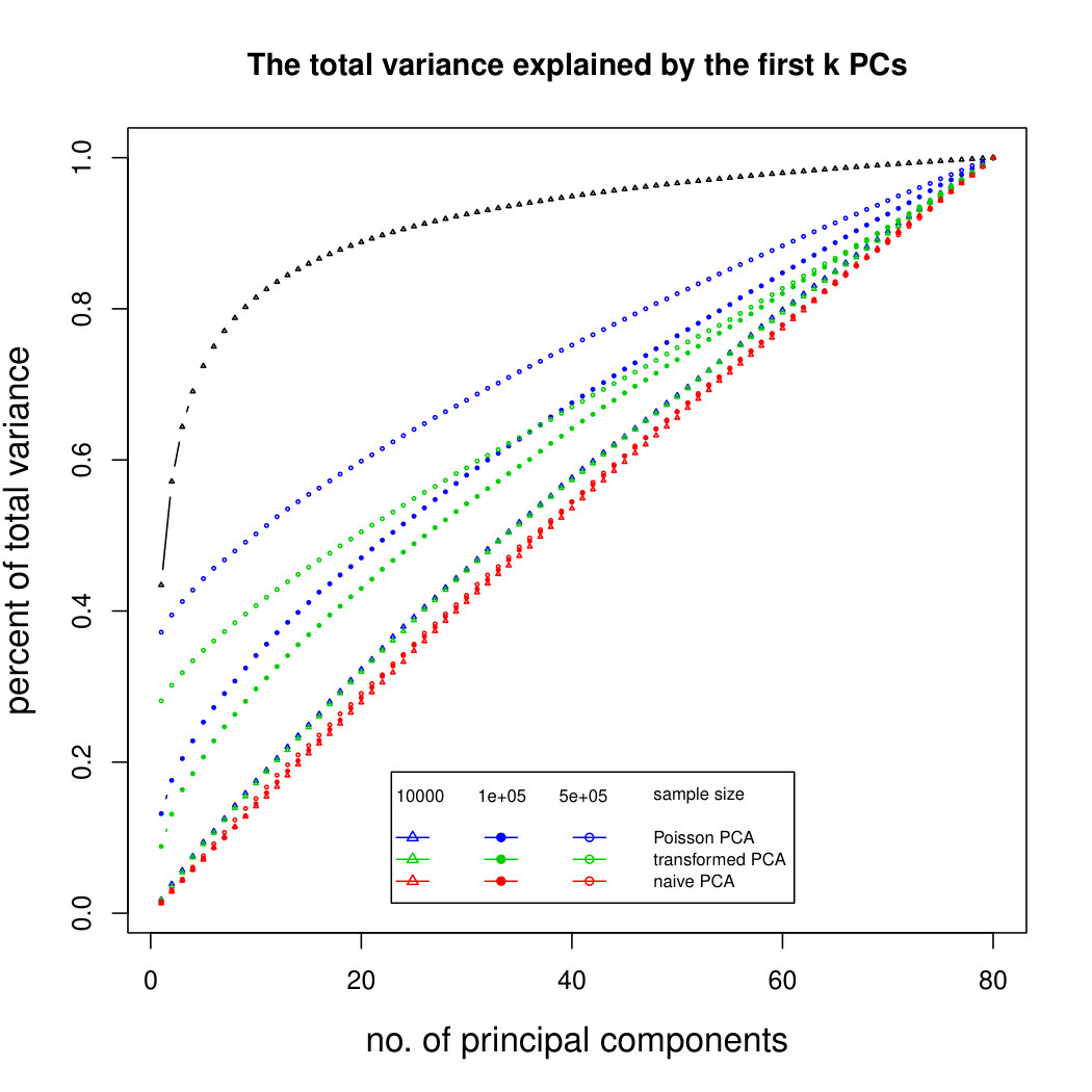 Figure 37
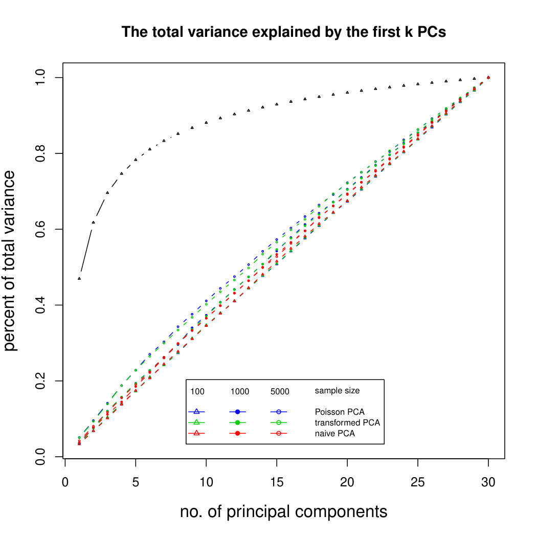 Figure 38
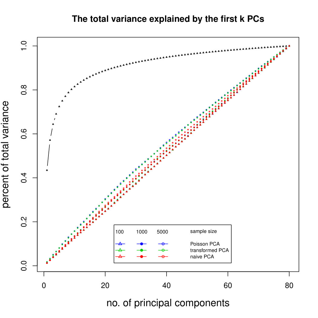 Figure 39
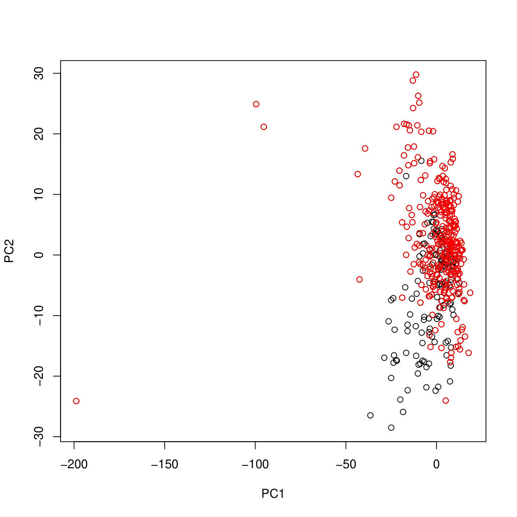 Figure 40
Peer Reviews
No public reviews on file for this paper yet. If you reviewed it on a platform where reviews are public (OpenReview, ICLR, NeurIPS, ICML), you can paste yours below so the community can read it here.
Videos
No videos yet. Explain this paper in a talk, walkthrough, or lecture? Add one.
Poisson PCA: Poisson Measurement Error corrected PCA, with Application
to Microbiome Data
Toby Kenney, Tianshu Huang The authors gratefully acknowledge funding from NSERC
Hong Gu
Department of Mathematics and Statistics, Dalhousie University The authors gratefully acknowledge funding from NSERC
Abstract
In this paper, we study the problem of computing a Principal Component Analysis of data affected by Poisson noise. We assume samples are drawn from independent Poisson distributions. We want to estimate principle components of a fixed transformation of the latent Poisson means. Our motivating example is microbiome data, though the methods apply to many other situations. We develop a semiparametric approach to correct the bias of variance estimators, both for untransformed and transformed (with particular attention to log-transformation) Poisson means. Furthermore, we incorporate methods for correcting different exposure or sequencing depth in the data. In addition to identifying the principal components, we also address the non-trivial problem of computing the principal scores in this semiparametric framework. Most previous approaches tend to take a more parametric line. For example the Poisson-log-normal (PLN) model, approach. We compare our method with the PLN approach and find that our method is better at identifying the main principal components of the latent log-transformed Poisson means, and as a further major advantage, takes far less time to compute. Comparing methods on real data, we see that our method also appears to be more robust to outliers than the parametric method.
Keywords: Dimension reduction; Compositional data; Sequencing depth correction; Count data; Log-normal Poisson
1 Introduction
Principal component analysis (PCA) is a widely used dimension reduction and data exploration technique. It is particularly suited for real valued multivariate data analysis with the underlying assumption that the measurement error in the data is additive. This can be seen from the fact that one way to define the PCA is by minimizing the reconstruction error of the data by the first principal components with the objective function defined as squared error loss. For other types of data, this loss function can be natually extended to be the negative loglikelihood function. This can be most natually developed to the whole exponential family distribution, for example, Collins et al. (2001) and Chiquet et al. (2018) maximized the exponential family loglikelihood of the data by assuming a lower dimensional representation of the natural parameters through the canonical link functions. Such an approach can be deemed as totally parametric and thus is sensitive to the model assumptions, outliers and the choice of the dimension for the latent parameter space. To some extent, this is more a parametric modelling method instead of data exploration.
Our focus in this paper is to develop a new PCA method for count data by correcting Poisson measurement errors, especially for those data observed from the high throughput sequencing technologies. Measurement error is an important issue in statistical analysis, that occurs when we want to analyse some latent variable, but our attempts to measure the variable are subject to random error. Our framework is conceptually different from that of Collins et al. (2001) and Chiquet et al. (2018). A closely related approach is the work of Liu et al. (2018) who develop the same estimator in the untransformed case without sequencing depth noise, as we do, but then proceed to develop shrinkage estimators to improve performance, rather than deal with sequencing depth noise or transformations. We assume that the latent Poisson means do not lie exactly on a low-dimensional space, but instead follow some unknown distribution, and we wish to estimate the principal components of this distribution or of a non-linear transformation of this distribution. When no transformation is needed, a PCA on an unbiased estimate of the covariance matrix of the latent Poisson means is straightforward. When a non-linear transformation is applied on the latent Poisson means, our idea is to derive a non-linear transformation of the data from which an unbiased estimator of the covariance matrix of the transformed latent Poisson means can be derived and thus the PCA can be applied on this unbiased estimate of the covariance. Our motivation for extending our work to transformed latent Poisson means is that previous research suggests that a logarithmic scale is an appropriate way to study microbial abundance. This also makes sense from the point of view of differential equation models of species abundance, which tend to imply exponential-type growth. We have avoided any parametric constraints on this latent distribution. Although our research is driven by the application to microbiome data which we will describe in more detail in the following subsection, the method is geneally applicable to high dimensional count data which are popularly observed in many different areas including social science, ecology, microbiology and bioscience in general.
The structure of the paper is as follows. In Section 2, we introduce the features of microbiome data which motivated this research. In Section 3, we develop the bias corrected estimators for the covariance matrices of functions of the latent Poisson means. Then in Section 4 we develop methods for handling the sequencing depth issue, particularly in the -transformed case. In Section 5, we provide a method for projecting the data onto the principal component space. We then demonstrate the performence of our methods on simulated data in Section 6 and on a real microbiome data set (Caporaso et al, 2010) in Section 7. Finally in Section 8, we summarise our work and suggest promising directions for future research.
The methods in this paper are all implemented in the R package PoissonPCA, which is available from the first author’s website www.mathstat.dal.ca/~tkenney/PoissonPCA/, and will be submitted to CRAN.
2 Features of microbiome data
The microbiome is the collection of all microorganisms in a particular environment. This collection mostly consists of bacteria, archaea, eukaryotes and viruses. Recent improvements in technology have allowed the bacteria and archaea components to be measured en-masse. That is, identifying DNA from all bacteria and archaea present in a given sample can be collected and counted, with the objective of giving a complete picture of the whole microbial community. This picture can then be compared to metadata, such as whether the microbial community was from a healthy individual or from an individual suffering from a particular illness. The idea is that the interaction of the thousands of microbes present in the whole community may be more informative than simple analyses that try to attribute complex conditions to the actions of a single species. There have been a large number of papers that have identified associations between the microbiome and various environmental conditions such as nutrient abundance (Arrigo 2005), and human health (Fujimura et al. 2010, Sekirov et al. 2010) including obesity (Turnbaugh et al. 2009), Crohn’s disease (Quince et al. 2013), diabetes (Kostic et al. 2015).
The microbiome data present a number of interesting data analysis challenges that make the application of PCA difficult. The feature of microbiome data that is the focus of this paper is measurement error. While each environment has a community with a certain total abundance of each Operational Taxonomic Unit (OTU), we only observe a small sample from that community, which for this paper, we will model as following a Poisson distribution with mean given by the underlying total abundance. In practice the sequencing procedure is more complicated (there are several different sequencing procedures that can be used, each of which involves their own noise and bias — Gorzelak et al. (2015) give more details about how the sequencing procedure influences the data) but the Poisson noise error seems a reasonable starting point. The aim of this paper is to adapt PCA to account for this Poisson measurement error.
A further feature of microbiome data is sequencing depth. Essentially, the issue is that the Poisson means of our observed sample are subject to large multiplicative noise. For this reason, microbiome data is usually treated as compositional data, with only the proportions of each OTU considered, for example Li (2015). However, this loses a lot of information about the Poisson distribution. For the Poisson distribution, the relative noise in the observed proportions will decrease as sequencing depth increases, so samples at higher sequencing depth should be given more weight. Another commonly used approach to the sequencing depth problem is rarefaction, where large parts of the data are thrown away, so that all samples have the same total OTU count. This practice is mainly due to the use of arbitrary indices which are sensitive to sample size. McMurdie and Holmes (2014) argue strongly against the use of rarefaction.
The other features of microbiome data include the high dimensionality and sparsity. There is substantial literature on ways to deal with these issues by imposing sparsity constraints on the PCA. For example Zou et al. (2006), and Jolliffe et al. (2003). Salmon et al. (2014) combine the Poisson PCA of Collins et al. (2001) with an penalty to create a sparse Poisson PCA, and apply this method to Photon-limited image denoising. However, the sparseness issue is not the focus for the current paper, and we will avoid it by grouping our OTUs at a higher taxonomic level, i.e. instead of considering variables that roughly correspond to the abundance of a particular species of microbe, we will look at higher-level variables that correspond to the total abundance of a whole genus or higher taxonomic level. This will reduce the dimension enough to avoid the curse of dimensionality for the datasets we consider. In principle the penalty could be applied to our method to provide a sparse Poisson-error corrected PCA, but that is a topic for future work.
There has been other work incorporating the Poisson error structure of microbiome data into the analysis, but it has been focused on parametric modelling, rather than Exploratory data analysis. For example Holmes et al. (2012) model microbiome data as a Dirichlet multinomial distribution; Knights et al. (2011) use a Bayesian mixture model; Shafiei et al. (2014) and Shafiei et al. (2015) develop hierarchical Bayesian multinomial mixture models; and Cai et al. (2017) apply non-negative matrix factorisation with Poisson error.
3 Method
We express the situation more formally as follows: We have samples of a -dimensional random vector which follows a Poisson distribution with conditional mean given by a latent random vector and a “sequencing depth” (this comes from our specific application to microbiome data). That is, we have , ’s are conditionally independent given the random vector and the sequencing depth . can be thought of as with some Poisson measurement error. Our samples form an matrix of observed data, where the th row is an independent sample of the random vector . We want to estimate the distribution of and its relationship to other variables. For this purpose, we develop a method of estimating a PCA on this latent , or on some transformation of , . Our approach to this problem is moment-based — we aim to correct the bias in the variance estimates, and use the unbiased variance estimates to perform PCA.
We start with the linear case, where we want to estimate the PCA of . There are two cases to consider: the case without sequencing depth noise (where for all ), and the case where sequencing depth correction is needed. We then develop the methods for estimating the PCA of a nonlinear transformation .
3.1 Poisson Noise Correction in PCA without Sequencing Depth Corrections
We first consider the simplest case, where for all . That is, any differences in total abundance between samples is a result of differences in underlying latent abundances. The model here is fairly straightforward. Latent Poisson means are a random vector , and observed counts are a random vector with conditionally independent given . We want to estimate the principal components of the random vector from a matrix whose rows are independent samples of the random vector . The principal components of are the eigenvectors of the variance of the vector , so we only need to provide an estimate for the variance of the random vector . We have
[TABLE]
where is a diagonal matrix with entries . Now we have the following straightforward estimators for and :
[TABLE]
plugging these in gives the estimator
[TABLE]
3.2 Poisson Noise Correction in PCA with Sequencing Depth Corrections
Suppose we now add sequencing depth noise to the problem, so that the Poisson mean is , where is a random scalar and is a random vector. To avoid the identifiability issue we assume , and that and are independent. We can apply the same procedure
[TABLE]
Thus
[TABLE]
Now since , , we have
[TABLE]
Thus
[TABLE]
We can now empirically estimate this quantity from a sample. Suppose we have a matrix , where each row is a sample from the underlying distribution of . If the sequencing depth is known, then we can compute for each sample, and we have empirical estimators
[TABLE]
where is a diagonal matrix with entries the sequencing depths of each observation. Plugging this into our formula for gives us the estimator
[TABLE]
The correction here is similar to the correction in (Li, Palta and Shao, 2004), where they added a correction term to the likelihood term in a regression model, where ’s are the Poisson samples, and ’s are the sequencing depths. Their case is a regression model, and in their case the sequencing depth is more directly observed (being number of hours of sleep).
3.3 Poisson PCA on Transformed Poisson Means without Sequencing Depth Corrections
Suppose now that we are interested in the covariance matrix of some transformation , where is some univariate function applied elementwise to . For example, we might set . We can use the same technique as in Section 3.1, but with some univariate transformation of the original data. Using the law of total variance, we have:
[TABLE]
Now if we can find so that then we get
[TABLE]
The first step, therefore is finding such that . Without loss of generality, we take as univariate. We can directly calculate as follows:
[TABLE]
That is, we can take to be the coefficients of the Taylor series of . As an example, suppose we want to give an unbiased estimator for for some fixed . We have
[TABLE]
We therefore get our estimator , which is a well-known unbiassed estimator for .
Next we need to calculate the conditional variance . Since the elements of are conditionally independent given , this matrix is a diagonal matrix and it will suffice to take as univariate for the estimation of each element of this matrix. We can estimate this from first principles:
[TABLE]
where is the coefficient of the Taylor series . Since is latent, we need to replace the expressions and by estimators which are functions of . Since we will be taking the expectation of our estimators of the conditional variance, it makes sense to focus on the bias of these estimators. For , there is an unbiassed estimator
[TABLE]
which can reasonably be used. This also has a computational advantage because it results in only needing to compute a single term in the sum. For the term , the unbiassed estimator is
[TABLE]
This gives us the overall estimator for the variance of , where is an element of the vector .
[TABLE]
The estimates of the off-diagonal elements of the covariance matrix can be computed as the corresponding elements of the sample covariance matrix of , where is applied elementwise to the observed data matrix .
In Appendix A, we show the consistency of this estimator:
Theorem 3.1**.**
If is a globally convergent Taylor series, is a non-negative random variable with finite raw moments and converges, then the estimator (1) is consistent.
In practice, this estimator can have high variance, leading to poor finite-sample performance for certain transformations. Sometimes this issue can be alleviated by using suitable approximations, and simplifying the algebra in equation (1). We show how this can be done for the commonly used log transformation in Appendix B. We also suggest a possible approach to the more general case, that could be given further study in Appendix C.
3.4 The Special Case of Log Transformation
In the special case when , the approach from Section 3.3 does not work, because does not have a globally convergent Taylor series. We can compute a Taylor series for for some value of . That is, we get
[TABLE]
This Taylor series is convergent for , however, when we expand the terms and try to reorganise it as a power series in , the coefficients do not converge. Therefore, we can only use a truncated power series. That is, we truncate the above series at some chosen value , to get a polynomial. This produces a reasonable approximation to on the interval . For larger values of , we have that . Therefore, we set instead for larger values of . The result of this is that for not too close to zero. In summary our function is given by
[TABLE]
There is some difficulty choosing the values of and . From experiments, we see that and whenever , gives a fairly good estimator. We discuss the corresponding estimator for conditional variance in Appendix B.
4 Sequencing Depth Correction
The methods described above for variance estimators of transformed latent Poisson means cover the situation without sequencing depth correction. In this section, we give two approaches to correcting the resulting covariance matrix for sequencing depth.
4.1 Method 1: Compositional Covariance Matrix for Sequencing Depth Correction
The first method is to get a compositional covariance matrix. That is, suppose the estimated covariance matrix is . We want to find the matrix with the following properties:
For any with , we have 2. 2.
is symmetric. 3. 3.
Conditions 2 and 3 are necessary for to be the covariance matrix of compositional data. Condition 1 says that the covariance matrices and give the same covariance for the projection of onto the space orthogonal to the vector . Now to solve this, we have the following.
Proposition 4.1**.**
The matrix that satisfies Conditions 1–3 is given by
[TABLE]
where .
Proof.
We first note that for any with , we have for some scalar . This is because for any with . By linearity, is a linear function of , so we have for some fixed vector . Now we have for all with . If we let , then this gives because is the orthogonal projection of onto the 1-dimensional space spanned by 1. Therefore we have where . Thus we have so Since and are both symmetric, we get , which gives the form in the proposition. All that now remains is to find the value of . This is forced by which gives
[TABLE]
∎
We have that , so solving for and we get that , so
[TABLE]
4.2 Method 2: Minimum Variance by Correcting for the Maximum Sequencing Depth Noise
The second method is specific to the case. In this case, the sequencing depth becomes additive noise on , proportional to the vector 1. This means that . The value of is not identifiable, but it is limited by the constraint that should be non-negative definite. One natural choice is therefore to select the largest value of such that remains non-negative definite. In the case where is an eigenvector of , this will give exactly the same result as the compositional method. In other cases, the results may differ slightly.
To solve for the largest value of such that is non-negative definite, we consider the determinant as a continuous function of . While is positive definite, the determinant is positive. We therefore set to be the smallest solution to . We solve this with a change of basis where is an orthogonal matrix with , where . Now we have that
[TABLE]
where is the matrix with the first row and column removed and the first entry replaced by . For example, if
[TABLE]
then
[TABLE]
More formally where is the first column of . This gives
[TABLE]
This gives us that
[TABLE]
where is the compositional estimate from Section 4.1. So we are trying to solve for such that
[TABLE]
Thus
[TABLE]
In practice, this method does not perform well, because the small eigenvalues and eigenvectors are not well estimated. Indeed some of the estimates are often negative. We therefore improve practical performance by introducing some thresholding. Let where
[TABLE]
with . Since should be non-negative definite, we first replace any negative eigenvalues by 0. Next we choose the smallest such that . The idea here is that we assume that is influenced mostly by sequencing depth and take eigenvalues accounting for 90% of the variance we are trying to estimate. We now replace all smaller eigenvalues for by . We now have a new diagonal matrix
[TABLE]
Then we apply the above minimum variance sequencing depth correction procedure to .
5 Projection onto Principal Component Space
Having estimated the principal components of the latent Poisson means, the remaining problem is to “project” the observations onto this principal component space. The methods in this paper are based on a semiparametric framework. We are assuming that the latent Poisson means follow some unknown distribution, and are seeking to use non-parametric methods to estimate the principal components of this latent distribution. In this spirit, our projection method should be based on the same assumptions. We will assume for each observed point, that there is some latent random vector of Poisson means, and that we want to project these Poisson means onto the principal component space. In the non-latent variance of principal components, we have an observation , and we seek the projection in principal component space that minimises . In our case, we have a latent random vector , and have calculated the principal component space of . If we knew , we would seek the projection in the principal component space that minimises , where is the covariance matrix of . (Because the principal component space is spanned by eigenvectors of , it turns out that it is equivalent to take the projection that minimises .)
However, we do not observe directly, instead, we observe . We therefore simultaneously expect to be such that has high likelihood, and such that is close to the principal component space. We therefore create the objective function
[TABLE]
where is the vector whose th element is — that is it is the logarithm function applied elementwise to the vector . Note that because we have computed the covariance matrix of , there is a canonical choice of how to balance the two constraints, and we do not need a tuning parameter. If the latent variable is normal, then is the negative log-likelihood of the joint distribution of and (treating as parameters).
To solve this, we substitute the linear model where is the matrix of principal component vectors. That is . Suppose that our projection is onto the first principal components and let
[TABLE]
That is, is the vector of the first elements of . Then we have . In this basis, the objective function becomes
[TABLE]
where is the diagonal matrix of eigenvalues of , in the order corresponding to . The estimate for is therefore given by setting the derivative of this to zero. That is
[TABLE]
In the particular case where (evaluated elementwise) this equation becomes
[TABLE]
Differentiating again, the Hessian matrix for the case where is
[TABLE]
where Newton’s method now gives
[TABLE]
6 Simulation
6.1 Simulation Design
We assess the performance of the method under three different transformations — the default untransformed Poisson means, a polynomial transformation , and a logarithmic transformation. In each case, we set the eigenvalues of the covariance matrix to a fixed sequence , and simulate the eigenvectors uniformly. We now simulate the true transformed covariance matrix as , where is a diagonal matrix with diagonal entries . We simulate an data matrix of transformed Poisson means, where each row of is i.i.d. with a chosen distribution (usually multivariate normal) with covariance matrix . We compute the Poisson means from by . Finally, we simulate . For each scenario, we simulate 100 datasets. We use the same eigenvalues, but different eigenvectors in the 100 simulated covariance matrices. We also simulate different means for for each simulated dataset, using a normal distribution with mean 100 and standard deviation 15.
For simulations with sequencing depth correction, in the compositional case, we modify the above procedure by setting , and , with other eigenvectors in simulated orthogonally to 1. In the non-compositional case, simulate as above. In both cases, we then simulate sequencing depth noise following a gamma distribution with shape parameter 4 and scale parameter 100.
6.2 Simulation Results
6.2.1 Assessing Simulation Results
We want to devise a method to assess the performance of our corrected PCA on the simulated data. In this case, we have a true covariance matrix , where is orthogonal and is diagonal. The principal component matrix is defined by the property of simultaneously maximising for all , subject to being orthogonal. We have obtained an estimated covariance matrix with orthogonal and diagonal. We want to assess the performance of as an estimate for . Since our objective is to maximise the variance explained by the first principal components, we will measure this by comparing cumulative true variance explained by the first estimated principal components, i.e. the cumulative sums , with the true cumulative sum .
6.2.2 Simulation results for untransformed PCA without sequencing depth correction
The simulation results for normally distributed Poisson means without sequencing depth noise with data dimensions equal to 80 are shown in Figure 1. We compare the percentages of the total variance explained by the true eigenvectors, the eigenvectors found by our Poisson PCA method, and the eigenvectors found by “naive PCA” i.e. applying PCA directly to the observed data, without any correction for Poisson error. We see that when , our method is comparable with naive PCA, but as sample size increases, our method performs much better, as expected. For large , our method appears to be converging to the correct eigenvalues as , while uncorrected PCA is not improving with larger sample sizes, because of the bias. Similar results when are shown in Supplementary Figure LABEL:linearsimresultsp30.
6.2.3 Simulation results for Polynomial Transformed PCA without sequencing depth correction
Figure 2 shows the simulation results for polynomial-transformed Poisson means. Again, our method is comparable to other methods for small sample sizes, and converges towards the truth as sample size increases. In this case, the larger variance of the estimators means that covergence of our method is slower than in the untransformed case. However, Poisson PCA begins to outperform other methods for sample size around 5,000, which is a plausible sample size for some real data sets. Supplemental Figure LABEL:polynomialsimresultsp30 shows similar results for .
6.2.4 Simulation results for Log Transformed PCA without sequencing depth correction
Figure 3 compares Poisson PCA to PLNPCA (Chiquet et. al, 2018), which is a parametric method based on a Poisson log-normal assumption using a variational approximation to estimate the parameters by MLE, and to PCA directly performed on the log-transformed data (with 0 counts arbitrarily replaced by 0.1). We compare the methods on both log-normal and non log-normal Poisson means. For the non log-normal case, we simulated some data in polar coordinates with direction uniformly distributed over the sphere and radius distributed following a centred gamma distribution with shape and scale . The data were then stretched to have the proscribed variance. Similar results with are shown in Supplemental Figure LABEL:logsimresultsp30.
When sample size is small, Poisson PCA clearly outperforms both PLNPCA methods and the naive PCA on log-tranformed data in the first few dimensions which capture about 70% to 80% of the total variance. After this point, the total variance explained by naive PCA on log-tranformed data starts to get higher. Between the two PLNPCA methods, the full rank log-Normal Poisson PCA seems to outperform the log-normal Poisson model with rank chosen by BIC. When sample size is large () the Poisson PCA and two PLNPCA methods show comparable results and perform better than the naive PCA on log-tranformed data. In practice, when we use PCA, we aim in particular to identify the first few principal components, so better performance at identifying the earlier prinicipal components is a very strong asset of our method. All the methods are robust to changing the underlying distribution of the Poisson means. Results for are shown in Supplemental Figure LABEL:logsimresultsn5000; we do not give results for larger because of the computation time needed by PLNPCA.
In addition to the better identification of the early principal components, Poisson PCA also has a major advantage in computation time. Figure 4 compares the logarithm of the average processor time (amount of computation performed) over 100 simulated datasets, for the three methods. For the limited rank PLNPCA, with rank chosen by BIC, we compared all possible ranks. Limiting the rank would improve the runtime of this method, to make it more comparable to the direct PLNPCA estimate. Poisson PCA is faster than the likelihood-based method by an order of magnitude. The runtimes are approximately linear in , so we have shown regression lines. Our Poisson PCA method is not quite linear, probably because the singular value decomposition, performed after variance estimation, takes nonlinear time. Because Poisson PCA is much faster than the other methods, this nonlinearity is more apparent for our method.
6.2.5 Simulation results for untransformed PCA and log-transformed PCA with sequencing depth correction
Figure 5 compares Poisson PCA with compositional PCA (i.e. data are rescaled so each row has total 1, and PCA is applied to the rescaled data). The scaled Poisson means are compositional, and follow a multivariate normal distribution; but we have multiplied each Poisson mean by a random sequencing depth. Our semiparametric method has done better than compositional PCA at identifying the principal components.
Figure 6 shows the results for log-normal simulated data with sequencing depth noise. In the compositional log Poisson means simulation, we use the log of observed total counts as an offset in the parametric PLN model. We see that this is a challenging problem, but that our compositional sequencing depth correction method (from Section 4.1) offers a slight improvement over the PLNPCA method. We do not include larger sample sizes because of the computation time needed to fit the PLNPCA model. We also compare our two methods for correcting sequencing depth noise when the latent covariance matrix is not compositional. We see that the minimum variance approach (from Section 4.2) has not done well at identifying the first eigenvector, because it has not removed enough sequencing depth noise. However, retaining the signal in the direction 1 allows it to get improved results for later principal components. Overall it seems that in most circumstances it would be better to use the compositional method, but in rare cases where we are aiming to find a large number of principal components, it may be preferable to use the minimum variance approach. Additional simulation results are shown in Supplemental Figure LABEL:logsimresultsseqdepthsupplemental.
6.3 Projection onto Principal Component Space
We now test the performance of the projection method from Section 5 on simulated data. We use our standard log-normal Poisson simulation without sequencing depth correction. We compare two projection approaches: (a) pure normal error — we take the log of the observed data and project this onto the principal component space (substituting for ); (b) the combined likelihood method from Section 5. We apply each of these projections both using the true covariance matrix, and using the estimated covariance matrix from Poisson PCA.
For assessing the quality of our projection, we have the true transformed Poisson mean , so we can project this Poisson mean onto the principal component space, and measure the distance between the correct projection and the estimated projection. Since the projection is orthogonal, Euclidean distance suffices for this measure.
Figure 7 compares the results on both the true principal component space, and the estimated principal component space. We see that when we project onto the true principal component space, our projection method outperforms the naïve projection method for all numbers of principal components. When we project onto the estimated principal component space, we see that our method performs excellently for any projection that might ever be used in practice. However, when we try to project onto high dimensional component spaces, our method starts to perform less well. In this case, because there is very little signal in the remaining dimensions, our method may soak up some of the noise. Optimisation is also more challenging in higher dimensions, so inaccuracies in the optimisation may cause deterioration in performance. Since the typical use of PCA is to obtain a low-dimensional representation of the data, performance on small numbers of principal components is most important. Therefore, the results of our method are good. Similar results for are in Supplementary Figure LABEL:ProjectionSimulationResultsp30.
7 Real Data Analysis
7.1 The Moving Picture Dataset
The moving picture dataset (Caporaso et al. 2011) is a large temporal microbiome dataset comprising samples from 4 body sites of two individuals over a period of approximately two years. There are over 300 samples from each site for individual 2 and over 100 samples from each site for individual 1. Previous analysis of this dataset has shown that it is relatively easy to distinguish the two individuals from the species-level OTUs, but using higher-level OTUs to distinguish them is more difficult. We apply our Poisson PCA method across a range of levels from phylum to genus from this dataset. Besides making the problem challenging compared to the results of previous studies, the focus on higher level OTUs also ensures that the number of variables is less than the number of observations, which is a necessary condition for the consistency of classical PCA. We present the results for the first two principal components at the order level (225 variables) in this section. Results at other levels are in the supplemenary materials.
There is substantial variation in sequencing depth between samples, with number of total reads varying between less than 10,000 and over 60,000. The distributions of sequencing depths were different for the two individuals. Since sequencing depth is largely considered noise due to experimental procedure, a method which separates samples based on sequencing depth is not a good method. To prevent methods that fail to correctly compensate for sequencing depth from wrongly seeming good, we used subsampling to ensure that the sequencing depths had the same distribution for each individual. (Details of the subsampling procedure are in Supplemental Appendix LABEL:RealDataSubsamplingProcedure.) We retain a large variability of sequencing depth within each individual’s samples, but remove the ability to use sequencing depth as a distinguishing feature, so that methods that better correct for sequencing depth noise are expected to perform better on the subsampled data.
7.2 Data Analysis
We compare three methods for dimension reduction of the log-transformed data: our compositional sequencing depth corrected Poisson PCA method using the projection method from Section 5; PLNPCA with rank chosen by BIC in the range 1–30, using total count as an offset; and log compositional PCA, i.e. naive PCA applied to the log of compositional data with zero counts replaced by 0.01 before converting to compositional data (similar results are obtained using other values to replace 0). Since the differences between the two individuals’ microbial communities are likely to be a large source of variability in the data, we expect to see a separation between samples from the two individuals after performing PCA on the data from each body site.
Results for the gut data are in Figure 8. We see that all three methods show a reasonable separation between the two individuals. PLNPCA shows several outliers, which can be explained by the difficulty of attempting to fit data to a prescribed parametric distribution if the distribution does not fit.
Figure 9 shows the projection of the tongue data. For this dataset, Poisson PCA shows a better separation between two individuals. PLNPCA has again been heavily influenced by a few outliers. Log compositional PCA shows a clear clustering, but the clustering is not related to the individual. Further examination reveals that the first principal component for both individuals is heavily influenced by a single order from phylum Cyanobacteria (see Supplementary Figure LABEL:Cyanobacteria). This applies to both Poisson PCA and log compositional PCA. However, it is more obvious in the case of log compositional PCA, and there is a clear gap between cases where the observed count of cyanobacteria is zero and where it is non-zero, which leads to the two clusters seen in Figure 9(a). The abundance of Cyanobacteria does not vary much between the two individuals, so because this abundance dominates the first principal component for log compositional PCA, we do not distinguish between the individuals using this method. Because Poisson PCA does not attach so much weight to the zero values, it is able to identify some signal, even with the Cyanobacteria abundance dominating the first principal component.
Figure 10 shows the results for the left palm. Previous research (e.g. Shafiei et al. 2015, Cai et al. 2016) has found these samples harder to classify than the gut or tongue data, so it is not surprising that all PCA methods show more mixing of the two groups. However, we see the same patterns as for the tongue data, with Poisson PCA producing the best separation, PLNPCA being adversely influenced by outliers and log compositional PCA producing a false clustering. This time, the false clustering can be seen to be closely related to sequencing depth (see Supplementary Figure LABEL:MovPicLPalmOrderSeqDepth).
Figure 11 shows the results for the right palm. Previous studies have found the right palms the most difficult locations to distinguish between the individuals, and the PCA results confirm this, with substantial mixing of the groups using all PCA methods, with log compositional PCA perhaps showing the best separation (certainly the best linear separation).
8 Conclusions and Future Work
8.1 Conclusions
We have developed methods for correcting for Poisson measurement error in estimating the variance of a latent variable. Our methods can estimate the variance of the latent Poisson means, or the variance of some transformation of the latent means. We have also incorporated ways to adjust our methods to deal with additional multiplicative noise in the Poisson means (sequencing depth). We have tested our methods across a range of scenarios and compared them with existing methods. We found that our method performs well on both simulated and real data, and is not so heavily influenced by outliers as parametric methods, and successfully adjusts for sequencing depth unlike naïve PCA on the logarithm of the compositional data.
While our method has focused on Poisson noise, so is less broad than some parametric methods that extend to exponential family distributions, our work is broader in that it can be applied to arbitrary transformations of the data, not just the logarithm. The ideas behind our work should easily be applicable to other families of noise distribution, particularly discrete. We have also developed methods for dealing with sequencing depth, that are not available in other methods. Furthermore, our method is an order of magnitude faster than parametric methods, because it does not require optimisation of all parameters.
8.2 Future Work
There are a number of avenues for extending this research. Firstly, for the log transformation, we were not able to find a perfect unbiased estimator, and instead used an approximation. Further work to find a better approximation and corresponding estimators should lead to better performance of the method. Secondly, while we have focussed on Poisson measurement error correction, the same ideas could be applicable to other measurement error correction for PCA. Our method was based on the fact that the Poisson distribution has one parameter, so the measurement error variance can be directly estimated from the data. This technique could be applied to other single parameter measurement error distributions. Thirdly, Liu et al. (2018) used shrinkage methods to improve the finite-sample performance of the untransformed Poisson PCA estimators; similar ideas could be applied to improve the finite sample performance of the sequencing depth corrected estimators and the transformed estimators. Finally, a large area of research in PCA is the implementation of sparseness constraints. Since our method provides an unbiassed variance estimator for the Poisson means, it should be straightforward to implement a standard regularisation method to ensure consistency in the case.
Appendix A Proof of Consistency of Transformed Variance Estimator
Theorem** (3.1).**
If is a globally convergent Taylor series, is a non-negative random variable with finite raw moments and converges, then the estimator (1) is consistent.
Proof.
Since the estimator (1) is unbiassed, the strong law of large numbers tells us that this is a consistent estimator provided and are both finite. We have
[TABLE]
which must be finite since otherwise the variance of which we are trying to estimate will not be finite.
We have that
[TABLE]
We are given that converges, so by Fubini’s theorem,
[TABLE]
is also finite. ∎
Appendix B Estimating Conditional Variance
We are interested in the logarithm case, so for large , we have . We now want to estimate . We will estimate it by taking the average of some function for each . That is, we want to design a function such that
[TABLE]
We will assume that is relatively large. We note that
[TABLE]
For large , we have that is almost certain to be much less than 1, so we can use the Taylor expansion
[TABLE]
We truncate this at the th term, for some , then we have
[TABLE]
We can truncate this again at (i.e. remove all powers of larger than ) to get
[TABLE]
Now we compute
[TABLE]
where is a Stirling number of the second kind. The second last equation comes from setting , and the last equation comes from setting . We have that is the number of partitions of a set of size into blocks with chosen singleton blocks. This gives us that
[TABLE]
is the number of partitions of with blocks and no singletons, since for any partition into blocks, of which are singletons, this partition is included times in the th term in the series (once for each subset of singletons). Therefore the total term assigned to this partition is
[TABLE]
We will denote the number of partitions with blocks and no singletons by . We therefore have
[TABLE]
We now substitute this into Equation (2) (noting that for , we have , and for , we have ) to get:
[TABLE]
Recall that is an estimator for , so substituting in this estimator gives us the estimator as
[TABLE]
where
[TABLE]
Our Poisson PCA package truncates at . The terms can be precalculated once for all data points, so computation of is quick.
Appendix C Alternative Estimator for Conditional Variance
Recall that the general estimator for conditional variance of a transformation depends on computing an estimator for for an integer . The unbiased estimator for this quantity is . However, this estimator can have very high variance, resulting in poor finite-sample performance. For the special case , we computed a useable approximation in Appendix B. For the general transformation case, we do not have a good general method. In this section, we suggest one possible approach that could be further studied.
The idea is to try to find two observations, and with the same value of . Then we have
[TABLE]
as an estimator for . We can then average this estimator over all pairs of values of and that come from approximately the same value of .
In practice we don’t know whether two values and come from the same value of . We therefore weight all pairs by how plausible it is that they have the same value of . We use the weight derived from the likelihood ratio statistic:
[TABLE]
and take the weighted average of divided by to get the estimator of .
That is, our estimator is
[TABLE]
The reference list from the paper itself. Each links out to its DOI / PubMed record.
- 1[1] Arrigo, K. (2005) Marine microorganism and global nutrient cycles Nature 437 , 349–355.
- 2[2] Cai, Y., Gu, H., Kenney, T. (2017). Learning Microbial Community Structures with Supervised and Unsupervised Non-negative Matrix Factorization. Microbiome 5 , 110.
- 3[3] Caporaso, J. G., Lauber, C. L., Costello, E. K., Berg-Lyons, D., Gonzalez, A., Stombaugh, J., Knights, D, Gajer, P., Ravel, J., Fierer, N., et al. (2011) Moving pictures of the human microbiome. Genome biology , 12(5):R 50.
- 4[4] Chiquet, J., Mariadassou, M., Robin, S. (2018) Variational Inference for Probabilistic Poisson PCA Ar Xiv:1703.06633 v 5 .
- 5[5] Collins, M., Dasgupta, S., Schapire, R.E. (2001). A generalization of principal components analysis to the exponential family. Advances in Neural Information Processing Systems 14 , 617–624.
- 6[6] Fujimura, K., Slusher, N., Cabana, M. and Lynch, S. (2010). Role of the gut microbiota in defining human health. Expert review of anti-infective therapy 8 , 435–454.
- 7[7] Gorzelak, M.A., Gill, S. K., Tasnim, N., Ahmadi-Vand, Z., Jay, M., and Gibson, D. L. Methods for improving human gut microbiome data by reducing variability through sample processing and storage of stool. Plo S one 10 e 0134802, 2015.
- 8[8] Holmes, I., Harris, K., Quince, C. (2012). Dirichlet multinomial mixtures: Generative models for microbial metagenomics. P Los One 7 30126.