Rapid evaluation of the spectral signal detection threshold and Stieltjes transform
William Leeb

TL;DR
This paper presents fast algorithms for evaluating spectral signal detection thresholds and the Stieltjes transform in large data matrices with heteroscedastic noise, aiding spectral denoising in statistical applications.
Contribution
The authors develop novel, provably correct algorithms for computing spectral thresholds and Stieltjes transforms in complex noise models, improving speed and accuracy over existing methods.
Findings
Algorithms are faster and more accurate than previous methods.
Validated performance through numerical experiments.
Applicable to models with separable variance profiles.
Abstract
Accurate detection of signal components is a frequently-encountered challenge in statistical applications with low signal-to-noise ratio. This problem is particularly challenging in settings with heteroscedastic noise. In certain signal-plus-noise models of data, such as the classical spiked covariance model and its variants, there are closed formulas for the spectral signal detection threshold (the largest sample eigenvalue attributable solely to noise) for isotropic noise in the limit of infinitely large data matrices. However, more general noise models currently lack provably fast and accurate methods for numerically evaluating the threshold. In this work, we introduce a rapid algorithm for evaluating the spectral signal detection threshold in the limit of infinitely large data matrices. We consider noise matrices with a separable variance profile (whose variance matrix is rank…
Click any figure to enlarge with its caption.
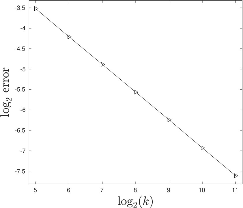 Figure 1
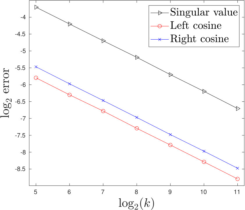 Figure 2
| err() | ||
|---|---|---|
| 1 | 2.08e-01 | 4.26e-02 |
| 2 | 4.34e-02 | 1.11e-02 |
| 3 | 2.55e-03 | 6.90e-04 |
| 4 | 9.66e-06 | 2.63e-06 |
| 5 | 1.40e-10 | 3.80e-11 |
| 6 | -2.75e-16 | -1.23e-16 |
| err() | ||
|---|---|---|
| 1 | -3.77e-01 | 3.71e-02 |
| 2 | -6.89e-02 | 8.34e-03 |
| 3 | -3.40e-03 | 4.34e-04 |
| 4 | -9.24e-06 | 1.18e-06 |
| 5 | -6.84e-11 | 8.73e-12 |
| 6 | -5.55e-15 | 7.85e-16 |
| err() | ||
|---|---|---|
| 1 | 1.25e+00 | -3.10e-01 |
| 2 | 3.10e-01 | -1.03e-01 |
| 3 | 3.12e-02 | -1.15e-02 |
| 4 | 3.92e-04 | -1.46e-04 |
| 5 | 6.34e-08 | -2.37e-08 |
| 6 | 2.00e-15 | -2.11e-16 |
| ) | err() | |
|---|---|---|
| 1 | 4.71e-01 | -1.00e+00 |
| 2 | 8.86e-03 | -1.93e-02 |
| 3 | 6.42e-06 | -1.40e-05 |
| 4 | 3.43e-12 | -7.50e-12 |
| 5 | 4.44e-16 | -1.10e-15 |
| Timing, | Timing, | |
|---|---|---|
| 18 | 4.30e-01 | 1.93e-01 |
| 19 | 8.67e-01 | 4.27e-01 |
| 20 | 1.89e+00 | 1.66e+00 |
| 21 | 3.95e+00 | 4.20e+00 |
| 22 | 8.41e+00 | 1.02e+01 |
| 23 | 1.70e+01 | 2.09e+01 |
| 24 | 3.43e+01 | 4.19e+01 |
| Error | Bias | |
|---|---|---|
| 5 | 8.73e-02 | 7.72e-02 |
| 6 | 5.41e-02 | 4.75e-02 |
| 7 | 3.39e-02 | 2.93e-02 |
| 8 | 2.12e-02 | 1.82e-02 |
| 9 | 1.32e-02 | 1.13e-02 |
| 10 | 8.20e-03 | 6.97e-03 |
| 11 | 5.12e-03 | 4.32e-03 |
| sing. val. | left cos. | right cos. | |
|---|---|---|---|
| 5 | 7.68e-02 | 1.80e-02 | 2.26e-02 |
| 6 | 5.43e-02 | 1.27e-02 | 1.59e-02 |
| 7 | 3.85e-02 | 9.10e-03 | 1.13e-02 |
| 8 | 2.74e-02 | 6.38e-03 | 7.98e-03 |
| 9 | 1.92e-02 | 4.53e-03 | 5.61e-03 |
| 10 | 1.36e-02 | 3.20e-03 | 3.99e-03 |
| 11 | 9.58e-03 | 2.25e-03 | 2.81e-03 |
| Alg. 3 | Min. | |
|---|---|---|
| 18 | 2.67e-01 | 2.38e-02 |
| 19 | 5.29e-01 | 4.63e-02 |
| 20 | 1.14e+00 | 1.30e-01 |
| 21 | 2.43e+00 | 3.20e-01 |
| 22 | 5.37e+00 | 6.94e-01 |
| 23 | 1.09e+01 | 1.38e+00 |
| 24 | 2.18e+01 | 2.73e+00 |
Peer Reviews
No public reviews on file for this paper yet. If you reviewed it on a platform where reviews are public (OpenReview, ICLR, NeurIPS, ICML), you can paste yours below so the community can read it here.
Videos
No videos yet. Explain this paper in a talk, walkthrough, or lecture? Add one.
Rapid evaluation of the spectral signal
detection threshold and Stieltjes transform
William Leeb111School of Mathematics, University of Minnesota, Twin Cities. Minneapolis, MN, USA.
Abstract
Accurate detection of signal components is a frequently-encountered challenge in statistical applications with low signal-to-noise ratio. This problem is particularly challenging in settings with heteroscedastic noise. In certain signal-plus-noise models of data, such as the classical spiked covariance model and its variants, there are closed formulas for the spectral signal detection threshold (the largest sample eigenvalue attributable solely to noise) for isotropic noise in the limit of infinitely large data matrices. However, more general noise models currently lack provably fast and accurate methods for numerically evaluating the threshold.
In this work, we introduce a rapid algorithm for evaluating the spectral signal detection threshold in the limit of infinitely large data matrices. We consider noise matrices with a separable variance profile (whose variance matrix is rank one), as these arise often in applications. The solution is based on nested applications of Newton’s method. We also devise a new algorithm for evaluating the Stieltjes transform of the spectral distribution at real values exceeding the threshold. The Stieltjes transform on this domain is known to be a key quantity in parameter estimation for spectral denoising methods. The correctness of both algorithms is proven from a detailed analysis of the master equations characterizing the Stieltjes transform, and their performance is demonstrated in numerical experiments.
1 Introduction
Random matrix theory is an increasingly popular tool for deriving methods in statistical signal processing applications. Recent applications include signal denoising [41], [18], [29], [33], [31], covariance estimation [16], [31], filter correction in signal and image processing [4], [14], multiple-input multiple-output (MIMO) wireless communication [8], [5], and factor analysis [15], [13], to name just a few.
Part of the appeal of random matrix theory is that for many classes of random matrices, certain random quantities of statistical significance converge to well-defined limits as the matrix size grows infinitely large. By way of introduction, we illustrate this phenemonon in the spiked covariance model, introduced by Johnstone in [24]. Here, the user observes iid random vectors in of the form , where (the signal component) is a random vector with covariance of rank and eigenvalues , and (the noise component) is a zero mean Gaussian vector with covariance . Typically, the user wishes to estimate quantities related to the signal covariance , such as its rank, eigenvectors, and eigenvalues, from the signal-plus-noise observations .
It is well-known that when and are both large, there emerge simple relationships between the sample covariance (where denotes the sample mean) and the signal covariance . For example, the largest eigenvalues of converge almost surely to the following limits as and :
[TABLE]
Furthermore, the inner products between the top eigenvectors of and the top eigenvectors of converge almost surely to the following limits:
[TABLE]
Proofs of these relationships may be found in the seminal work [38], while extensions to more general noise models can be found in [3]. These relationships have been used to devise estimators of , as in the work [16], as well as to predict the signal vectors themselves, as in [41], [18], [29], [30].
Of particular significance for the present work is the value . This is the limiting value of the operator norm of the sample covariance of the noise component alone as and ; see [19]. More generally, for any sequence of random noise matrices whose operator norms have an almost sure asymptotic limit as the dimensions grow to infinity, we refer to that limiting value as the spectral signal detection threshold, or SSDT for short. As is apparent for white noise from the formula (1), observed eigenvalues exceeding the SSDT may be attributed to the signal component, and used to extract information about the signal. Eigenvalues below the SSDT are not as useful for recovering information on the signal (though see Remark 4 below). In typical applications of the spiked covariance model and its generalizations to signal denoising, only the eigenvalues of exceeding the SSDT are used for denoising [18], [16], [30], [33], [14], [31], [4]. For this reason, evaluation of the SSDT is a critical task in statistical signal processing.
While the SSDT and related quantities, such as the relations between the eigenvalues of and , have simple formulas in the case of white noise, more general noise models pose greater challenges. In this paper, we study a fairly broad family of noise matrices, namely those with a separable variance profile: every entry of the noise matrix has a potentially different variance, but the matrix of all the variances is rank one. This type of random matrix arises naturally in a number of applications, such as signal denoising with variable-strength heteroscedastic noise and the Kronecker model of multiple-input multiple-output transmission. We show that even when there are not closed formulas for the quantities of interest in this model, they may nevertheless be evaluated rapidly and to machine precision via provably correct algorithms.
1.1 This paper’s contributions
This paper introduces fast, scalable, and numerically stable algorithms for two related problems arising in statistical signal processing applications. The first is to evaluate the spectral signal detection threshold (SSDT) for noise matrices with a separable variance profile. As explained above, the SSDT is the asymptotic value of the operator norm of a random matrix representing the noise component in a signal-plus-noise observation model as the dimensions of the matrix grow to infinity.
The second problem we address is evaluating the Stieltjes transform (also known as the Cauchy-Stieltjes transform) of a certain probability measure associated with the noise matrix, known as the limiting spectral distribution (LSD). The Stieltjes transform is a function of central interest in random matrix theory and its applications; we recall its precise definition in Section 2.1. As we will review in Section 2.3, the Stieltjes transform, evaluated at real values exceeding the SSDT, may be used to estimate certain model parameters and perform signal denoising. Like the SSDT itself, in isotropic noise the Stieltjes transform has a closed form, while more general variance profiles pose greater challenges which we address in the current paper.
The algorithms we present scale linearly with the number of problem parameters, and are provably accurate to machine precision. The solution and analysis of each problem makes use of the master equations characterizing the Stieltjes transform, which will be reviewed in Section 2.2. Through a detailed analysis, presented in Section 3, we prove that the desired values may be computed by the use of Newton’s root-finding algorithm. For the SSDT, several intermediate quantities used in each iteration of Newton’s method are themselves computable by Newton’s method, as we will show. Consequently, all parameters we compute are either available analytically, or can be provably computed to full precision by a rapidly converging iterative scheme. For matrices of size -by-, the asymptotic costs of the algorithms scale like .
1.2 Relation to prior work
The signal-plus-noise matrix models of the kind we consider have been previously studied in the statistical literature, in works such as [24], [3], [33], [14], [31], [18], [38], [30], [16], [22], [20], [49], [21]. Estimating the number of signal terms in such principal components analysis and factor models is a well-studied problem in statistics and statistical signal processing applications [15], [13], [6], [23], [25], [37], [26]. Detection in the low SNR regime constitutes a distinct though conceptually relevant class of problems in signal processing [44], [46], [47], [48]. Noise matrices with separable variance profiles have also been studied in the context of the Kronecker product model for MIMO wireless communication [8], [5] and factor analysis with applications to economics [35]. We also note that such random matrices are a special case of “algebraic” random matrices, introduced in [40].
The solution to both of the problems we study rests on a known characterization of the Stieltjes transform of the LSD as the solution to a set of certain non-linear equations; these have appeared in [39] and [9]. We present a new, detailed analysis of these equations. As a consequence of our analysis, we show that evaluating the Stieltjes transform may be done by a straightforward application of Newton’s root-finding algorithm, whereas the SSDT is computable by several nested applications of Newton’s agorithm, appropriately initialized.
Previous works have considered the problem of evaluating the LSD, its Stieltjes transform, and the boundary of its support, for different classes of random noise matrices. The paper [12] proposes a scheme for evaluating the Stieltjes transform at complex values outside the support of the LSD; this method is based on a non-linear equation satisfied by the Stieltjes transform [42], [43], [32]. The method in [7] is devoted to extending the approach to mixture models. The papers [27], [28] are concerned with solving the inverse problem of recovering the population distribution from the observed spectrum; this problem is also taken up in [17]. The paper [15] contains a method for finding the boundary of a certain family of LSDs based on root-finding, although the use of Newton’s method is not employed or analyzed. To the best of our knowledge, the problem of evaluating the SSDT and Stieltjes transform for random matrices with a separable variance profile has not been addressed in prior work; and for special cases that have been studied, such as in [15], the prior work does not contain fast algorithms with the guarantees presented here.
1.3 Outline
The remainder of the paper is outlined as follows. In Section 2, we precisely state the problems we solve in this paper, and review the mathematical and numerical material that we will be using. In Section 3, we derive the core mathematical theory on which our algorithms rest, namely a detailed analysis of the master equations characterizing the Stieltjes transform of the LSD. In Section 4, we provide explicit descriptions of the numerical algorithms for finding the SSDT and evaluating the Stieltjes transform. In Section 5, we present the results of several illustrative numerical experiments demonstrating the performance of our algorithms.
2 Preliminaries
2.1 Setting and problem formulation
We suppose we have a -by- random matrix of the form , where is a random matrix with iid entries of mean zero and variance , and and are positive-definite matrices of sizes -by- and -by-, respectively. We define the empirical spectral distribution (ESD) to be the distribution of eigenvalues of the matrix :
[TABLE]
As is typical in high-dimensional problems, we work in the asymptotic regime where and both grow to infinity. More precisely, we suppose that grows with , and that the limit
[TABLE]
is well-defined, positive, and finite. Furthermore, as and grow, we suppose that the eigenvalue spectra of and have well-defined asymptotic distributions and , respectively (in terms of weak convergence), with compact support. Under suitable conditions on and , the sequence of measures will almost surely converge weakly to a compactly supported measure , called the limiting spectral distribution (LSD). We also denote by the limiting spectral distribution of the eigenvalues of .
We define the spectral signal detection threshold (SSDT) as follows:
[TABLE]
This is the right endpoint of the LSD ’s support, or equivalently the asymptotic operator norm of the matrix . As we will explain in Section 2.3, in a signal-plus-noise model where is a low-rank signal matrix, eigenvalues exceeding are attributable to the signal .
Next, we define the Stieltjes transform of :
[TABLE]
which has derivative equal to
[TABLE]
Similarly, the Stieltjes transform of is given by
[TABLE]
with derivative equal to
[TABLE]
We call the associated Stieltjes transform of . The functions and are defined for all complex outside the supports of and , respectively. However, as we will explain in Section 2.3, in the present work we are only interested in evaluating , , and their derivatives for real .
In this paper, we consider the setting where and are discrete distributions of the form
[TABLE]
and
[TABLE]
Here, and are positive numbers, and the weights and satisfy , , and . For example, if eigenvalues of are 1, and the remaining are equal to 2, then , , , and .
With this background and notation, we can concisely state the two problems we solve in this paper:
Problem 1. Given with corresponding weights ; and with corresponding weights ; evaluate the SSDT .
Problem 2. Given with corresponding weights ; and with corresponding weights ; and a value ; evaluate , , , and .
Algorithms solving Problems 1 and 2 to machine precision, with asymptotic cost , are presented in Section 4.
Remark 1**.**
In the problem statements, the parameters , , , and are user-supplied inputs. In many statistical applications, these parameters are assumed to be known, as in the works [15], [31], [12], [22], [20], [21].
Remark 2**.**
The assumption that and are discrete measures is quite common in the literature on random matrix theory and its applications [15], [31], [12], [22], [20], [21]. It is likely that the methods in the present work can be generalized to more general measures, so long as certain linear functionals of the measures can be efficiently computed (e.g. by numerical quadrature). Pursuing this in detail lies outside the scope of the current work, however.
2.2 Properties of the Stieltjes transform
The Stieltjes and associated Stieltjes transforms of the LSD are defined by equations (6) and (8), respectively. We refer the reader to the standard references [1], [45] for a detailed treatment of Stieltjes transforms of probability measures, particularly random spectral measures.
Lemma 1**.**
The Stieltjes transforms and satisfy the following relations:
[TABLE]
and
[TABLE]
Lemma 2**.**
The derivatives and satisfy the following relations:
[TABLE]
and
[TABLE]
Lemma 2 follows from Lemma 1, which in turn follows immediately from the relation:
[TABLE]
Remark 3**.**
Lemmas 1 and 2 show that and may be easily evaluated once and are computed.
The next result is central to our subsequent analysis.
Theorem 1**.**
The Stieltjes transform for the LSD satisfies the following master equations:
[TABLE]
where
[TABLE]
and is a function that satisfies the equation
[TABLE]
For a proof of Theorem 1, see, for instance, the paper [39]. The paper [9] presents a slightly modified form of these equations, with a detailed analysis showing that is smooth for real outside the support of .
We assume that and are discrete measures of the form
[TABLE]
and
[TABLE]
where , , and . The master equations therefore become:
[TABLE]
where is a function satisfying
[TABLE]
and the function is defined by:
[TABLE]
We note that in the case where (the singly-weighted case), the master equations take on a simpler form; see, for instance, [43], [42].
2.3 Spiked models and the -transform
In a spiked matrix model, we observe a signal-plus-noise matrix of the form
[TABLE]
where is a rank signal matrix, and is a noise matrix. The -transform is defined as follows:
[TABLE]
where and are, respectively, the Stieltjes transform and associated Stieltjes transform of the LSD of . The -transform was introduced in [3], though as a function of rather than .
Denoting by the top eigenvalues of , and , the corresponding left and right singular vectors of , respectively, it is shown in [3] that the -transform defines a mapping between and the eigenvalues of the signal matrix , which holds almost surely in the limit :
[TABLE]
This is satisfied for sufficiently large eigenvalues of , namely those for which . Phrased differently, an observed eigenvalue of satisfying may be attributed to the presence of signal.
Furthermore, the asymptotic cosines and , , can also be evaluated using the Stieltjes transform. It is shown that, almost surely,
[TABLE]
and
[TABLE]
Consequently, evaluating and provides a method for estimating the angles between the population singular vectors , and the observed singular vectors , . These relationships have been employed to derive optimal methods of singular value shrinkage [33].
Remark 4**.**
While eigenvalues of exceeding the SSDT indicate the presence of signal, the converse statement – if all eigenvalues are less than , then there is no signal – is subtler. For example, the work [36] studies the detection of signals in white noise and shows that the joint distribution of all eigenvalues of changes even when the signal eigenvalues do not exceed the SSDT. However, the resulting statistical test does not accurately distinguish between the presence or absence of signal with overwhelming probability. Regardless, in tasks such as covariance and signal estimation in the spiked model, only those eigenvalues exceeding the SSDT are typically used for covariance estimation and signal denoising [18], [16], [30], [33], [14], [31], [4].
Remark 5**.**
Separable variance profiles arise naturally when the columns of are independent random vectors in of the form
[TABLE]
where the are signal vectors constrained to an -dimensional subspace of ; is a positive definite matrix; and are specified weights. In this model, each signal vector is observed in the presence of heteroscedastic noise (with covariance ) of variable strength . The noise matrix alone is distributed like , where . Models like these are considered in, for example, [30], [11]. When , this model is considered in [22], [20], [21]; when , this model is considered in [49], [31].
Proposition 1**.**
For , is decreasing and convex.
Proof.
Write , where and . Using and , and and for , it is enough to show that are increasing and concave. But this follows immediately from the identities
[TABLE]
and
[TABLE]
and the definitions (6) and (8) of and . ∎
2.4 Newton’s root-finding algorithm
Newton’s method is a classical technique for finding the roots of a function of one real variable. We briefly review the method here; the reader may consult any standard reference on optimization or numerical analysis, such as [34], [10], for additional details. We are given a smooth function , where , and we suppose and . We also suppose that and for all ; that is, is a strictly increasing and concave. Our goal is to compute , the unique root of in .
To find , Newton’s method initializes , and defines a sequence of updates recursively as follows: given an estimate , the next value is defined by
[TABLE]
Geometrically, is the root of the line tangent to the graph of at the point . Because is concave, it is easy to see that .
Because each is obtained from a linear approximation to , the errors decay quadratically in the vicinity of ; that is
[TABLE]
when is sufficiently small.
Remark 6**.**
Quadratic convergence is what makes Newton’s method an especially attractive algorithm when it is applicable – that is, when both and may be accurately evaluated, and exhibits the conditions specified above. In practical terms, quadratic convergence means that the number of accurately computed digits of approximately doubles after each iteration of the algorithm, until machine precision is reached.
3 Mathematical apparatus
In this section, we analyze the master equations (22) – (24). Our results will provide the necessary tools to devise algorithms for computing the SSDT and evaluating and for . We define
[TABLE]
and
[TABLE]
We define the function by:
[TABLE]
Then for each , satisfies . When we treat as a fixed parameter and as a variable, we will use the notation .
3.1 Range and monotonicity of when
We first state a result on the range of for . The function approaches [math] as , and grows to as , and is strictly decreasing on the interval
[TABLE]
For any , we define the interval by
[TABLE]
Proposition 2**.**
When , is contained in the interval .
We will develop the proof in several steps.
Lemma 3**.**
Let . Then the function is bounded for all .
Proof.
We show that the range of cannot approach any of the singularities of , which lie at the values . Define
[TABLE]
Then from (22)
[TABLE]
and consequently
[TABLE]
Since is bounded for , this tells us that must stay bounded so long as is bounded away from [math]; in particular, cannot be made arbitrarily close to any of the singularities . ∎
Corollary 1**.**
* as .*
Proof.
Because is bounded for large , the result follows from (23). ∎
Corollary 2**.**
For any , ; that is,
[TABLE]
Proof.
This follows from the continuity of for , and the facts that it never passes through and approaches 0 at large . ∎
Corollary 3**.**
For all , and .
Proof.
The positivity of follows immediately from Corollary 2. The negativity of then follows from (42), and the fact that . ∎
Lemma 4**.**
For all ,
[TABLE]
Proof.
We have , from (22). Suppose for some , we had
[TABLE]
The inequality must then remain true for all sufficiently large , since is continuous and does not pass through . However, the left side converges to [math] as , since is bounded for large ; a contradiction. This completes the proof. ∎
We have shown that for all , lies in the interval defined by the inequalities
[TABLE]
This completes the proof of Proposition 2.
Next we prove that is increasing:
Proposition 3**.**
The function is increasing for .
Proof.
We have:
[TABLE]
Since , we have:
[TABLE]
and so
[TABLE]
Consequently, can never be [math]. Furthermore,
[TABLE]
which converges to 1 as (note that stays bounded away from singularities of and also , which have the same singularities). So for sufficiently large , and hence, since it is continuous and cannot pass through 0, for all . ∎
3.2 Behavior of
In this section we characterize the behavior of (viewed as a function of ) on the interval . Specifically, we show the following. For any , is a strictly convex function that approaches as approaches either end of . Furthermore, when , the minimum value of is less than zero, and ; consequently, there are exactly two roots of , both contained in the interval . We show that is always equal to the largest root, namely the one at which .
Lemma 5**.**
For , the function is strictly convex on ; that is, .
Proof.
We have:
[TABLE]
and
[TABLE]
Now whenever , we have for all , and for all ; consequently,
[TABLE]
and
[TABLE]
Consequently, for all , i.e. the function is convex. ∎
Lemma 6**.**
The function diverges to as and as approaches the left endpoint of from the right.
Proof.
This is immediate from the definition of . ∎
Lemma 7**.**
For each , .
Proof.
We have:
[TABLE]
Since and is decreasing on , and , we also have ; consequently, . ∎
Proposition 4**.**
For , .
Proof.
This follows from (49) and . ∎
We have shown that has two roots in the interval whenever . Proposition 4 identifies as the root that is closest to zero, or equivalently, the root where the derivative of is positive. This characterization will be used in Section 4.2 to devise the algorithm for computing , and consequently .
3.3 The minimum of
We will let denote the minimum of on ; that is, is the unique value on that satisfies
[TABLE]
We define the function for by:
[TABLE]
For any , we define the function for by:
[TABLE]
Note that by definition, for all .
We will show that is decreasing and convex and is increasing and concave.
Lemma 8**.**
* is a decreasing function of .*
Proof.
The derivative of may be computed as follows:
[TABLE]
which is negative. ∎
Proposition 5**.**
* is a convex function of .*
Proof.
We first compute the derivative of . We have
[TABLE]
Differentiating with respect to , we find
[TABLE]
and so
[TABLE]
Now the second derivative of is given by
[TABLE]
We will show that for all . In fact, we will show the stronger result that each summand is positive, or equivalently, recalling that ,
[TABLE]
To prove this, we observe that
[TABLE]
To show that this is less than 1, it is enough to show that
[TABLE]
or equivalently
[TABLE]
We will show that this inequality holds for any value of between [math] and . If , then the right side becomes
[TABLE]
and since the term
[TABLE]
is positive (because is convex, , and on ), the desired inequality is satisfied.
On the other hand, if , the right hand side becomes
[TABLE]
where the inequality holds since , and for all . By the Cauchy-Schwarz inequality,
[TABLE]
or in other words,
[TABLE]
This gives the desired result. ∎
Proposition 6**.**
For all , is an increasing and concave function of .
Proof.
The first derivative of is:
[TABLE]
which as we’ve seen is positive. The second derivative of is
[TABLE]
which is always negative, since , , , and for all and . ∎
4 Algorithms
In this section, we describe the algorithms for computing the SSDT and for evaluating the Stieltjes transform and its derivative at values . By Lemmas 1 and 2, and may be easily found from and .
4.1 Computation of the boundary
In this section, we derive an algorithm for the computation of . First, we observe that when , then as we have shown there are real roots of to the left and to the right of ; in particular, . On the other hand, if , the function cannot have a real root, since that would imply that the Stieltjes transform is real inside the support of . Consequently, . It follows that the SSDT is the value at which ; that is, , is the unique root of on .
From Lemma 8 and Proposition 5, is decreasing and convex. With an efficient procedure for evaluating and , we can therefore use Newton’s algorithm to find its root if we initialize the algorithm to the left of the root. In Section 4.1.2, we detail how to evaluate and . As a preliminary step, we will need to compute the left endpoint of ; we do this in 4.1.1. The resulting algorithm for evaluating is summarized in Algorithm 3.
4.1.1 Computation of the left endpoint of ,
We recall the definition of the interval :
[TABLE]
where is the interval . Let us denote by the left endpoint of . Since is a decreasing function of on , is the unique root of
[TABLE]
on . Since is a decreasing, convex function of on , we may find its root using Newton’s algorithm, initialized to the left of the root. Such an initial value can be found by starting with any value in , and performing bisection with , the left endpoint of , until we arrive at a value where . Newton’s algorithm is then performed with initial value . We summarize the procedure in Algorithm 1.
4.1.2 Evaluation of , , and
Next, we show how to evaluate the functions , , and . is defined as the root of on . Since is an increasing, concave function, we may find its root using the Newton algorithm initialized to the left of the root, i.e. the region where . Such an initial value may be found by taking a starting point to the right of , and performing bisection on and until we arrive at a value with . We can then perform Newton’s algorithm on , initialized at . The procedure is summarized in Algorithm 2.
4.2 Evaluation of and ,
In this section, we present an algorithm for evaluating the Stieltjes transform of , and its derivative , when . This immediately provides a method for evaluating and , and the -transform defined in Section 2.3.
As we showed in Section 3.2, the function is convex on and has two roots, both of which are negative. The root closest to [math], i.e. the rightmost root, is . Since and is convex, this tells us that Newton’s method, initialized at , will converge to . For brevity, we introduce the function defined by:
[TABLE]
With this notation, we have:
[TABLE]
and
[TABLE]
Note that from (48), we can evaluate :
[TABLE]
The method for evaluating and is summarized in Algorithm 4.
5 Numerical results
In this section, we report on several experiments illustrating the behavior of the algorithms from Section 4. For the timings reported in Sections 5.2 and 5.5, we used an implementation written in MATLAB 2019b and run on a Dell Precision 5540 with 62.5 GB of RAM and an Intel Core i9 CPU. The MATLAB code is available at the following URL: https://github.com/wleeb/MPBoundary.
5.1 Convergence
Algorithms 1 – 4 are all versions of the Newton root-finding method. In this section, we illustrate the quadratic convergence of these methods, as predicted from the theory reviewed in Section 2.4. In each experiment, we used parameters , , and . We generated the values and randomly from a distribution, and assigned random probabilities and by drawing values from and normalizing to sum to 1. For experiments in which a value is specified, we also choose it at random.
In Tables 1 – 4, the first column displays the iteration number , starting from the initial value and going until the root has been reached. The second column displays the function value at the iterate; the algorithm terminates when the function reaches machine precision . We work in double precision, so . The third column displays the relative error in the root itself, defined by:
[TABLE]
Table 1 shows the results for Algorithm 1, which computes the left endpoint of . Table 2 shows the results for Algorithm 2, which evaluates . Table 3 shows the results for Algorithm 3, which computes the boundary . Table 4 shows the results for Algorithm 4, which evaluates .
Remark 7**.**
For each algorithm, we observe quadratic convergence close to the root, as expected. That is, on each iteration close to termination the number of correct digits roughly doubles, and the size of the objective roughly squares, until machine precision is reached.
5.2 Scalability
In the next experiment, we compute timings for the computation of and the evaluation of . For increasing values of , we set (). We generated the values and randomly from a distribution, and assigned them random probabilities and by drawing values from and normalizing to sum to 1.
For each , we then record the time in seconds required to compute , and the time in seconds required to compute on a grid of 100 equispaced values of between and . The reported timings are averaged over five runs of the experiment, and are displayed in Table 5. It is apparent that the running times scale approximately linearly with , as we would expect. In addition to linearly scaling with , the magnitudes of the timings are quite encouraging; for example, it takes only about 4 seconds to compute when is over two million and is over one million.
5.3 Finite sample accuracy for
The master equations (22) – (24) from which we compute are asymptotic and deterministic, holding almost surely in the limit as . In this experiment, we assess the finite sample accuracy of estimating the SSDT from the operator norm of the random matrix . We consider how the estimate improves as and grow. We use a model where , and both and have point masses at and , each with weight ; and set . We generate matrices of size -by-, where grows and .
For each value of , we draw such a -by- random matrix and compute the operator norm of . We compare this to the value of computed using Algorithm 3. In Table 6, we show the mean absolute error, averaged over runs for each value of . More precisely, if is the operator norm of from trial , we record
[TABLE]
We also record the average bias, defined as
[TABLE]
In Figure 1, we plot the log error against . The plot demonstrates a linear dependence. The slope of the line is estimated to be approximately .
Remark 8**.**
In [24], it is shown that for white noise the expected fluctations of the top eigenvalue of are of the order , which implies the log-log plot would have a slope of . The observed slope of approximately is a close match to this value.
Remark 9**.**
For all values of , the bias is positive. In other words, the estimated values tend to underestimate .
5.4 Finite sample accuracy of spiked model parameters
In this experiment, we test the finite sample accuracy of parameter estimation in the spiked random matrix model. We consider -by- random matrices of the form , where is a rank “signal” matrix with uniformly random singular vectors and , and is a random Gaussian noise matrix with separable variance profile. We will denote by
As we reviewed in Section 2.3, the top eigenvalue of converges almost surely to a value satisfying , in the limit . Furthermore, if and are the top singular vectors of , then the absolute inner products and converge almost surely to and , respectively. We remind the reader that we define the -transform by .
We test the accuracy of these formulas for finite and increasing values of and . Using Algorithm 4 for evaluating and , we can easily evaluate . Proposition 1 shows that for a specified parameter , Newton’s root-finding algorithm may be used to solve for the asymptotic . The asymptotic values and are then evaluated from their respective formulas.
We compare these asymptotic values to the top eigenvalue of and the cosines between the singular vectors of and , for randomly generated data. We again use a model where , and both and have point masses at and , each with weight ; and set . We generate matrices of size -by-, where grows and . We generate a signal matrix where and are uniformly random unit vectors in and , respectively; and , ensuring a detectable signal.
For each value of , we draw such a -by- random matrix and compute the operator norm of . We compare this to the asymptotic value of . We also compare the values and to and , respectively. In Table 7, we show the mean absolute errors of these estimates, averaged over runs for each value of . More precisely, if is the operator norm of from trial , and and are the left and right cosines, respectively, we record the mean absolute errors:
[TABLE]
In Figure 2, we plot the log errors against . The plots all demonstrate a linear dependence. The slope of each line is estimated to be approximately .
Remark 10**.**
In [3], it is shown that the expected fluctations of the top eigenvalue of are of the order , which implies the log-log plot would have a slope of . In [2], it is shown that in the case of white noise the expected fluctations of the cosines are also of order , also leading to a slope of . Our observed slopes closely match these values.
5.5 One-sided weights
While Algorithm 3 computes the SSDT for an arbitrary separable variance profile, a special case of this problem that arises in certain applications is when ; that is, the variance profile has one-sided weights. In [15], it is shown that the SSDT may be evaluated by finding the minimizer of the function
[TABLE]
on the interval , and then setting . The minimizer is the unique root of the monotonic function
[TABLE]
on the interval .
When viable, this approach has obvious advantages over Algorithm 3, namely that it finds the root of a function which can be evaluated in closed form rather than by nested applications of Newton’s method. Properly applied, it should be substantially faster than Algorithm 3. However, the paper [15] does not analyze the behavior of the function (86), beyond observing that it is monotonic.
We compare the method from [15] for evaluating based on the minimizer of to Algorithm 3. To find the root of , we employ bisection until the error is approximately square root of machine epsilon, and then use Newton’s method to achieve full accuracy. In our experiment, we set , and for each value of we generate the ’s uniformly randomly on and take uniform weights . For each value of , we solve the problem using each method for runs, and average the timings of all the runs; the timings are presented in Table 8.
The results of the experiment are extremely encouraging. They suggest that for one-sided weights, working with the function (86) yields a substantially faster computation of the SSDT than the general master equations (22) – (24). However, a more detailed analysis of the function (86) must be carried out to justify such an approach and show that a fast algorithm is viable for general and ; this is beyond the scope of the current work.
6 Conclusion
We have introduced an algorithm for rapidly computing the spectral signal detection threshold in signal-plus-noise random matrix models. We have considered a class of random noise matrices with separable variance structure, which arise often in applications. Our algorithm is based on an implicit characterization of derived from the master equations for the Stieltjes transform . Several nested applications of Newton’s method are applied to evaluate and auxiliary parameters. Fast algorithms are also introduced to evaluate and , the Stieltjes transform and its derivative, at real values . We have demonstrated the rapid convergence of these methods and their linear scaling in numerical tests. We have also shown the effects of random fluctations for increasing values of and .
Acknowledgements
I acknowledge support from NSF BIGDATA award IIS 1837992 and BSF award 2018230. I thank Edgar Dobriban for helpful discussions and for pointing out the method from [15]. I also thank the reviewers for their helpful comments on the manuscript.
The reference list from the paper itself. Each links out to its DOI / PubMed record.
- 1[1] Zhidong Bai and Jack W. Silverstein. Spectral Analysis of Large Dimensional Random Matrices . Springer Series in Statistics. Springer, 2009.
- 2[2] Zhigang Bao, Xiucai Ding, and Ke Wang. Singular vector and singular subspace distribution for the matrix denoising model. The Annals of Statistics , 49(1):370–392, 2021.
- 3[3] Florent Benaych-Georges and Raj Rao Nadakuditi. The singular values and vectors of low rank perturbations of large rectangular random matrices. Journal of Multivariate Analysis , 111:120–135, 2012.
- 4[4] Tejal Bhamre, Teng Zhang, and Amit Singer. Denoising and covariance estimation of single particle cryo-EM images. Journal of Structural Biology , 195(1):72–81, 2016.
- 5[5] Ezio Biglieri, Robert Calderbank, Anthony Constantinides, Andrea Goldsmith, Arogyaswami Paulraj, and H. Vincent Poor. MIMO Wireless Communications . Cambridge University Press, 2007.
- 6[6] Andreas Buja and Nermin Eyuboglu. Remarks on parallel analysis. Multivariate Behavioral Research , 27(4):509–540, 1992.
- 7[7] Lucilio Cordero-Grande. MIXANDMIX: numerical techniques for the computation of empirical spectral distributions of population mixtures. Computational Statistics & Data Analysis , 141:1–11, 2020.
- 8[8] Romain Couillet and Merouane Debbah. Random Matrix Methods for Wireless Communications . Cambridge University Press, 2011.