Scene Graph Prediction with Limited Labels
Vincent S. Chen, Paroma Varma, Ranjay Krishna, Michael Bernstein,, Christopher Re, Li Fei-Fei

TL;DR
This paper presents a semi-supervised approach for scene graph prediction that effectively leverages limited labeled data and unlabeled images to improve relationship detection in visual knowledge bases.
Contribution
It introduces a novel probabilistic label generation method using heuristics and a factor graph model, enabling training of scene graph models with minimal labeled data.
Findings
Outperforms baseline methods by 5.16 recall@100 on PREDCLS
Effective with as few as 10 labeled examples per relationship
Relationship complexity correlates with method success (R^2=0.778)
Abstract
Visual knowledge bases such as Visual Genome power numerous applications in computer vision, including visual question answering and captioning, but suffer from sparse, incomplete relationships. All scene graph models to date are limited to training on a small set of visual relationships that have thousands of training labels each. Hiring human annotators is expensive, and using textual knowledge base completion methods are incompatible with visual data. In this paper, we introduce a semi-supervised method that assigns probabilistic relationship labels to a large number of unlabeled images using few labeled examples. We analyze visual relationships to suggest two types of image-agnostic features that are used to generate noisy heuristics, whose outputs are aggregated using a factor graph-based generative model. With as few as 10 labeled examples per relationship, the generative model…
Click any figure to enlarge with its caption.
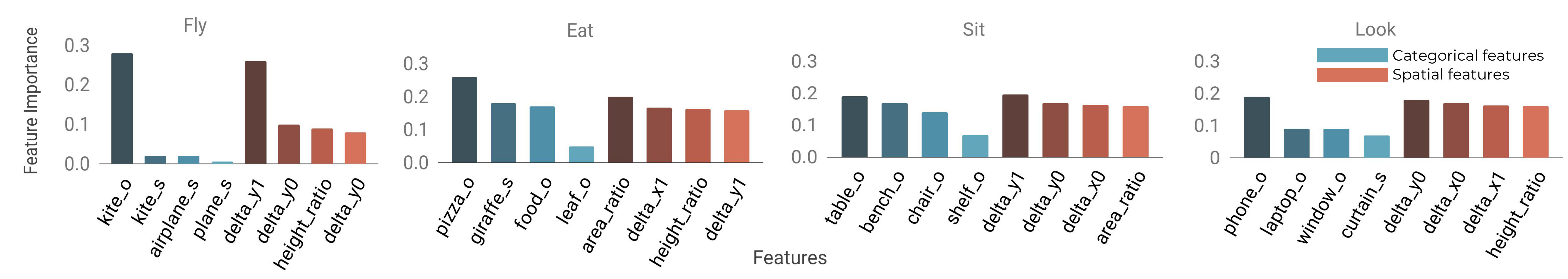 Figure 1
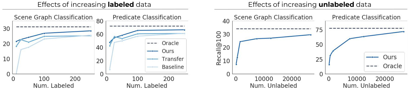 Figure 2
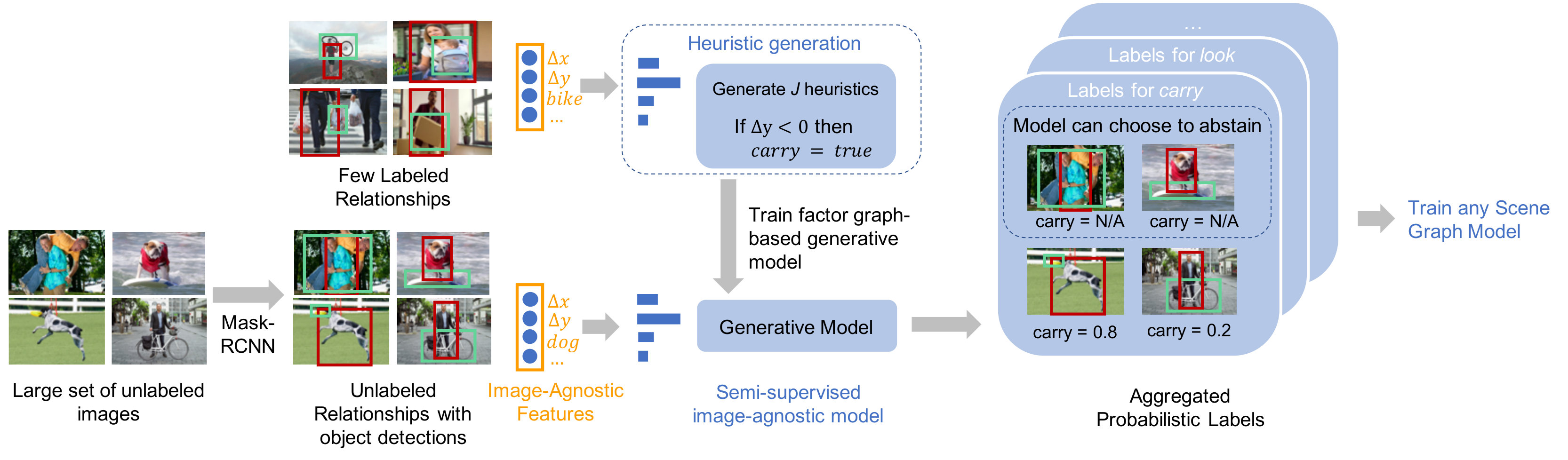 Figure 3
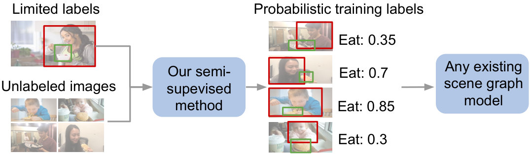 Figure 4
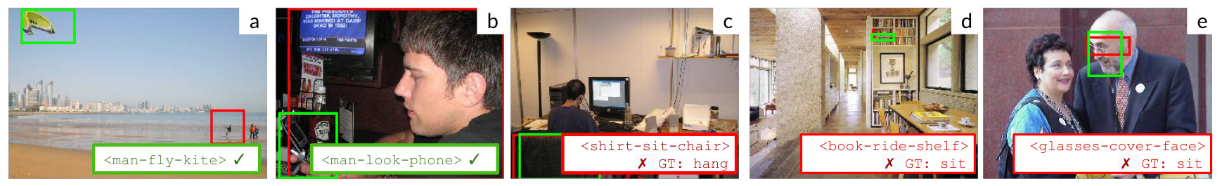 Figure 5
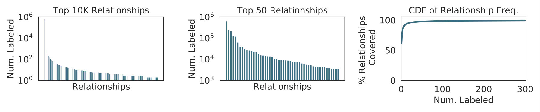 Figure 6
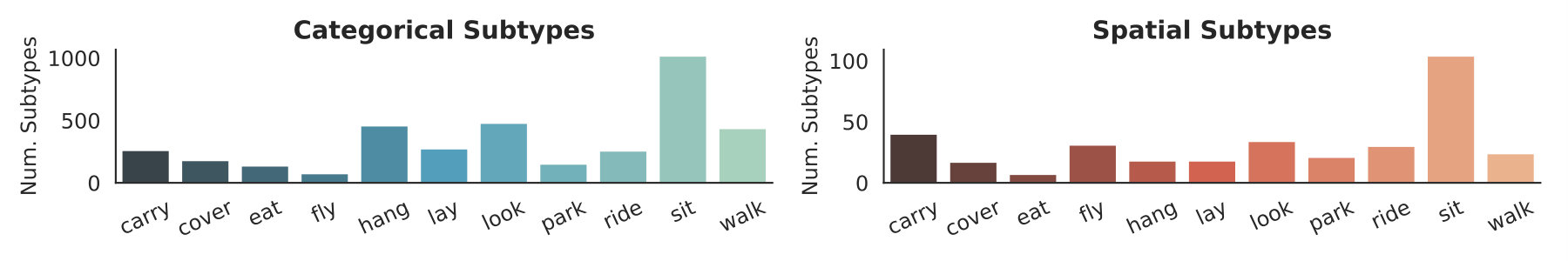 Figure 7
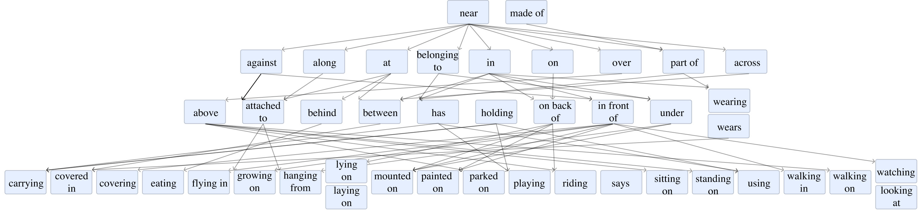 Figure 8
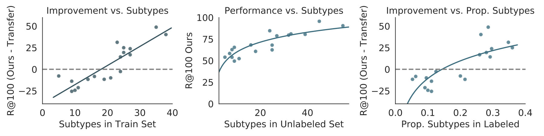 Figure 9
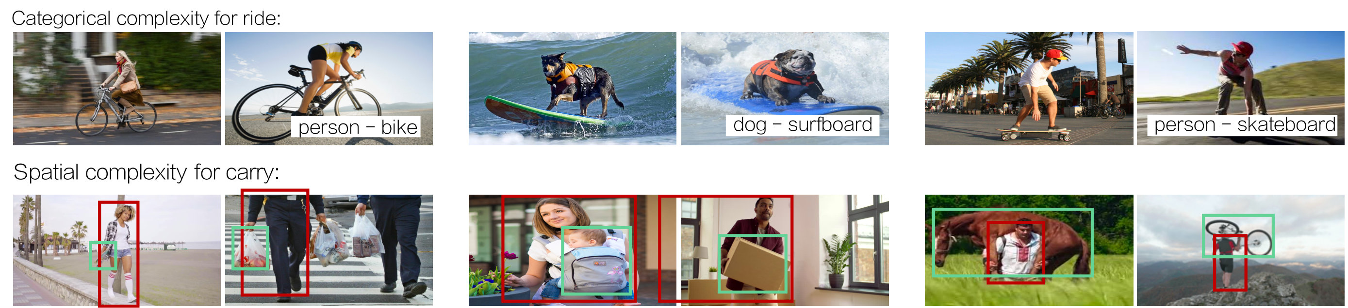 Figure 10
| Num. Labeled () | 200 | 175 | 150 | 125 | 100 | 75 | 50 | 25 | 10 | 5 |
|---|---|---|---|---|---|---|---|---|---|---|
| % Relationships | 99.09 | 99.00 | 98.87 | 98.74 | 98.52 | 98.15 | 97.57 | 96.09 | 92.26 | 87.28 |
| Model () | Prec. | Recall | F1 | Acc. |
|---|---|---|---|---|
| Random | 5.00 | 5.00 | 5.00 | 5.00 |
| Decision Tree | 46.79 | 35.32 | 40.25 | 36.92 |
| Label Propagation | 76.48 | 32.71 | 45.82 | 12.85 |
| Ours (Majority Vote) | 55.01 | 57.26 | 56.11 | 40.04 |
| Ours (Categ. + Spat.) | 54.83 | 60.79 | 57.66 | 50.31 |
| Scene Graph Detection | Scene Graph Classification | Predicate Classification | ||||||||||||
| Model | R20 | R50 | R100 | R20 | R50 | R100 | R20 | R50 | R100 | |||||
| Baselines | Baseline [] | 0.00 | 0.00 | 0.00 | 0.04 | 0.04 | 0.04 | 3.17 | 5.30 | 6.61 | ||||
| Freq | 9.01 | 11.01 | 11.64 | 11.10 | 11.08 | 10.92 | 20.98 | 20.98 | 20.80 | |||||
| Freq+Overlap | 10.16 | 10.84 | 10.86 | 9.90 | 9.91 | 9.91 | 20.39 | 20.90 | 22.21 | |||||
| Transfer Learning | 11.99 | 14.40 | 16.48 | 17.10 | 17.91 | 18.16 | 39.69 | 41.65 | 42.37 | |||||
| Decision tree [38] | 11.11 | 12.58 | 13.23 | 14.02 | 14.51 | 14.57 | 31.75 | 33.02 | 33.35 | |||||
| Label propagation [57] | 6.48 | 6.74 | 6.83 | 9.67 | 9.91 | 9.97 | 24.28 | 25.17 | 25.41 | |||||
| Ablations | Ours (Deep) | 2.97 | 3.20 | 3.33 | 10.44 | 10.77 | 10.84 | 23.16 | 23.93 | 24.17 | ||||
| Ours (Spat.) | 3.26 | 3.20 | 2.91 | 10.98 | 11.28 | 11.37 | 26.23 | 27.10 | 27.26 | |||||
| Ours (Categ.) | 7.57 | 7.92 | 8.04 | 20.83 | 21.44 | 21.57 | 43.49 | 44.93 | 45.50 | |||||
| Ours (Categ. + Spat. + Deep) | 7.33 | 7.70 | 7.79 | 17.03 | 17.35 | 17.39 | 38.90 | 39.87 | 40.02 | |||||
| Ours (Categ. + Spat. + WordVec) | 8.43 | 9.04 | 9.27 | 20.39 | 20.90 | 21.21 | 45.15 | 46.82 | 47.32 | |||||
| Ours (Majority Vote) | 16.86 | 18.31 | 18.57 | 18.96 | 19.57 | 19.66 | 44.18 | 45.99 | 46.63 | |||||
| Ours (Categ. + Spat.) | 17.67 | 18.69 | 19.28 | 20.91 | 21.34 | 21.44 | 45.49 | 47.04 | 47.53 | |||||
| Oracle [] | 24.42 | 29.67 | 30.15 | 30.15 | 30.89 | 31.09 | 69.23 | 71.40 | 72.15 | |||||
| Scene Graph Detection | Scene Graph Classification | Predicate Classification | |||||||||||
|---|---|---|---|---|---|---|---|---|---|---|---|---|---|
| Model | R20 | R50 | R100 | R20 | R50 | R100 | R20 | R50 | R100 | ||||
| Baseline [] | 1.06 | 1.80 | 2.66 | 4.70 | 6.00 | 5.43 | 9.63 | 12.17 | 13.07 | ||||
| Ours (Categ. + Spat.) | 4.04 | 6.75 | 8.64 | 12.69 | 13.91 | 14.16 | 24.72 | 27.76 | 28.53 | ||||
| Oracle [] | 14.20 | 20.61 | 25.44 | 33.58 | 35.52 | 35.92 | 62.00 | 66.92 | 68.02 | ||||
Peer Reviews
No public reviews on file for this paper yet. If you reviewed it on a platform where reviews are public (OpenReview, ICLR, NeurIPS, ICML), you can paste yours below so the community can read it here.
Code & Models
Videos
No videos yet. Explain this paper in a talk, walkthrough, or lecture? Add one.
Taxonomy
TopicsMultimodal Machine Learning Applications · Advanced Image and Video Retrieval Techniques · Video Analysis and Summarization
Scene Graph Prediction with Limited Labels
Vincent S. Chen, Paroma Varma, Ranjay Krishna, Michael Bernstein, Christopher Ré, Li Fei-Fei
Stanford University
{vincentsc, paroma, ranjaykrishna, msb, chrismre, feifeili}@cs.stanford.edu
Abstract
Visual knowledge bases such as Visual Genome power numerous applications in computer vision, including visual question answering and captioning, but suffer from sparse, incomplete relationships. All scene graph models to date are limited to training on a small set of visual relationships that have thousands of training labels each. Hiring human annotators is expensive, and using textual knowledge base completion methods are incompatible with visual data. In this paper, we introduce a semi-supervised method that assigns probabilistic relationship labels to a large number of unlabeled images using few labeled examples. We analyze visual relationships to suggest two types of image-agnostic features that are used to generate noisy heuristics, whose outputs are aggregated using a factor graph-based generative model. With as few as labeled examples per relationship, the generative model creates enough training data to train any existing state-of-the-art scene graph model. We demonstrate that our method outperforms all baseline approaches on scene graph prediction by {\color[rgb]{0,0,0}{5.16}} recall@100 for PREDCLS. In our limited label setting, we define a complexity metric for relationships that serves as an indicator () for conditions under which our method succeeds over transfer learning, the de-facto approach for training with limited labels.
1 Introduction
In an effort to formalize a structured representation for images, Visual Genome [27] defined scene graphs, a formalization similar to those widely used to represent knowledge bases [18, 13, 56]. Scene graphs encode objects (e.g. person, bike) as nodes connected via pairwise relationships (e.g., riding) as edges. This formalization has led to state-of-the-art models in image captioning [3], image retrieval [25, 42], visual question answering [24], relationship modeling [26] and image generation [23]. However, all existing scene graph models ignore more than of relationship categories that do not have sufficient labeled instances (see Figure 2) and instead focus on modeling the few relationships that have thousands of labels [49, 31, 54].
Hiring more human workers is an ineffective solution to labeling relationships because image annotation is so tedious that seemingly obvious labels are left unannotated. To complement human annotators, traditional text-based knowledge completion tasks have leveraged numerous semi-supervised or distant supervision approaches [7, 6, 17, 34]. These methods find syntactical or lexical patterns from a small labeled set to extract missing relationships from a large unlabeled set. In text, pattern-based methods are successful, as relationships in text are usually document-agnostic (e.g. Tokyo - is capital of - Japan). Visual relationships are often incidental: they depend on the contents of the particular image they appear in. Therefore, methods that rely on external knowledge or on patterns over concepts (e.g. most instances of dog next to frisbee are playing with it) do not generalize well. The inability to utilize the progress in text-based methods necessitates specialized methods for visual knowledge.
In this paper, we automatically generate missing relationships labels using a small, labeled dataset and use these generated labels to train downstream scene graph models (see Figure 1). We begin by exploring how to define image-agnostic features for relationships so they follow patterns across images. For example, eat usually consists of one object consuming another object smaller than itself, whereas look often consists of common objects: phone, laptop, or window (see Figure 3). These rules are not dependent on raw pixel values; they can be derived from image-agnostic features like object categories and relative spatial positions between objects in a relationship. While such rules are simple, their capacity to provide supervision for unannotated relationships has been unexplored. While image-agnostic features can characterize some visual relationships very well, they might fail to capture complex relationships with high variance. To quantify the efficacy of our image-agnostic features, we define “subtypes” that measure spatial and categorical complexity (Section 3).
Based on our analysis, we propose a semi-supervised approach that leverages image-agnostic features to label missing relationships using as few as labeled instances of each relationship. We learn simple heuristics over these features and assign probabilistic labels to the unlabeled images using a generative model [39, 46]. We evaluate our method’s labeling efficacy using the completely-labeled VRD dataset [31] and find that it achieves an F1 score of {\color[rgb]{0,0,0}{57.66}}, which is {\color[rgb]{0,0,0}{11.84}} points higher than other standard semi-supervised methods like label propagation [57]. To demonstrate the utility of our generated labels, we train a state-of-the-art scene graph model [54] (see Figure 6) and modify its loss function to support probabilistic labels. Our approach achieves 47.53 recall@100111Recall@ is a standard measure for scene graph prediction [31]. for predicate classification on Visual Genome, improving over the same model trained using only labeled instances by 40.97 points. For scene graph detection, our approach achieves within 8.65 recall@100 of the same model trained on the original Visual Genome dataset with more labeled data. We end by comparing our approach to transfer learning, the de-facto choice for learning from limited labels. We find that our approach improves by 5.16 recall@100 for predicate classification, especially for relationships with high complexity, as it generalizes well to unlabeled subtypes.
Our contributions are three-fold. (1) We introduce the first method to complete visual knowledge bases by finding missing visual relationships (Section 5.1). (2) We show the utility of our generated labels in training existing scene graph prediction models (Section 5.2). (3) We introduce a metric to characterize the complexity of visual relationships and show it is a strong indicator () for our semi-supervised method’s improvements over transfer learning (Section 5.3).
2 Related work
Textual knowledge bases were originally hand-curated by experts to structure facts [5, 44, 4] (e.g. Tokyo - capital of - Japan). To scale dataset curation efforts, recent approaches mine knowledge from the web [9] or hire non-expert annotators to manually curate knowledge [47, 5]. In semi-supervised solutions, a small amount of labeled text is used to extract and exploit patterns in unlabeled sentences [37, 34, 35, 33, 21, 2]. Unfortunately, such approaches cannot be directly applied to visual relationships; textual relations can often be captured by external knowledge or patterns, while visual relationships are often local to an image.
Visual relationships have been studied as spatial priors [14, 16], co-occurrences [51], language statistics [53, 31, 28], and within entity contexts [29]. Scene graph prediction models have dealt with the difficulty of learning from incomplete knowledge, as recent methods utilize statistical motifs [54] or object-relationship dependencies [49, 30, 50, 55]. All these methods limit their inference to the top most frequently occurring predicate categories and ignore those without enough labeled examples (Figure 2).
The de-facto solution for limited label problems is transfer learning [15, 52], which requires that the source domain used for pre-training follows a similar distribution as the target domain. In our setting, the source domain is a dataset of frequently-labeled relationships with thousands of examples [49, 30, 50, 55], and the target domain is a set of limited label relationships. Despite similar objects in source and target domains, we find that transfer learning has difficulty generalizing to new relationships. Our method does not rely on availability of a larger, labeled set of relationships; instead, we use a small labeled set to annotate the unlabeled set of images.
To address the issue of gathering enough training labels for machine learning models, data programming has emerged as a popular paradigm. This approach learns to model imperfect labeling sources in order to assign training labels to unlabeled data. Imperfect labeling sources can come from crowdsourcing [10], user-defined heuristics [8, 43], multi-instance learning [22, 40], and distant supervision [12, 32]. Often, these imperfect labeling sources take advantage of domain expertise from the user. In our case, imperfect labeling sources are automatically generated heuristics, which we aggregate to assign a final probabilistic label to every pair of object proposals.
3 Analyzing visual relationships
We define the formal terminology used in the rest of the paper and introduce the image-agnostic features that our semi-supervised method relies on. Then, we seek quantitative insights into how visual relationships can be described by the properties between its objects. We ask (1) what image-agnostic features can characterize visual relationships? and (2) given limited labels, how well do our chosen features characterize the complexity of relationships? With these in mind, we motivate our model design to generate heuristics that do not overfit to the small amount of labeled data and assign accurate labels to the larger, unlabeled set.
3.1 Terminology
A scene graph is a multi-graph that consists of objects as nodes and relationships as edges. Each object consists of a bounding box and its category where is the set of all possible object categories (e.g. dog, frisbee). Relationships are denoted subject - predicate - object or <$$o - - o^{\prime}$$>. is a predicate, such as ride and eat. We assume that we have a small labeled set of annotated relationships for each predicate . Usually, these datasets are on the order of a examples or fewer. For our semi-supervised approach, we also assume that there exists a large set of images without any labeled relationships.
3.2 Defining image-agnostic features
It has become common in computer vision to utilize pretrained convolutional neural networks to extract features that represent objects and visual relationships [49, 31, 50]. Models trained with these features have proven robust in the presence of enough training labels but tend to overfit when presented with limited data (Section 5). Consequently, an open question arises: what other features can we utilize to label relationships with limited data? Previous literature has combined deep learning features with extra information extracted from categorical object labels and relative spatial object locations [25, 31]. We define categorical features, , as a concatenation of one-hot vectors of the subject and object . We define spatial features as:
[TABLE]
where and are the top-left bounding box coordinates and their widths and heights.
To explore how well spatial and categorical features can describe different visual relationships, we train a simple decision tree model for each relationship. We plot the importances for the top spatial and categorical features in Figure 3. Relationships like fly place high importance on the difference in y-coordinate between the subject and object, capturing a characteristic spatial pattern. look, on the other hand, depends on the category of the objects (e.g. phone, laptop, window) and not on any spatial orientations.
3.3 Complexity of relationships
To understand the efficacy of image-agnostic features, we’d like to measure how well they can characterize the complexity of particular visual relationships. As seen in Figure 4, a visual relationship can be defined by a number of image-agnostic features (e.g. a person can ride a bike, or a dog can ride a surfboard). To systematically define this notion of complexity, we identify subtypes for each visual relationship. Each subtype captures one way that a relationship manifests in the dataset. For example, in Figure 4, ride contains one categorical subtype with person - ride - bike and another with dog - ride - surfboard. Similarly, a person might carry an object in different relative spatial orientations (e.g. on her head, to her side). As shown in Figure 5, visual relationships might have significantly different degrees of spatial and categorical complexity, and therefore a different number of subtypes for each. To compute spatial subtypes, we perform mean shift clustering [11] over the spatial features extracted from all the relationships in Visual Genome. To compute the categorical subtypes, we count the number of unique object categories associated with a relationship.
With access to or fewer labeled instances for these visual relationships, it is impossible to capture all the subtypes for given relationship and therefore difficult to learn a good representation for the relationship as a whole. Consequently, we turn to the rules extracted from image-agnostic features and use them to assign labels to the unlabeled data in order to capture a larger proportion of subtypes in each visual relationship. We posit that this will be advantageous over methods that only use the small labeled set to train a scene graph prediction model, especially for relationships with high complexity, or a large number of subtypes. In Section 5.3, we find a correlation between our definition of complexity and the performance of our method.
4 Approach
We aim to automatically generate labels for missing visual relationships that can be then used to train any downstream scene graph prediction model. We assume that in the long-tail of infrequent relationships, we have a small labeled set of annotated relationships for each predicate (often, on the order of a examples or less). As discussed in Section 3, we want to leverage image-agnostic features to learn rules that annotate unlabeled relationships.
Our approach assigns probabilistic labels to a set of un-annotated images in three steps: (1) we extract image-agnostic features from the objects in the labeled and from the object proposals extracted using an existing object detector [19] on unlabeled , (2) we generate heuristics over the image-agnostic features, and finally (3) we use a factor-graph based generative model to aggregate and assign probabilistic labels to the unlabeled object pairs in . These probabilistic labels, along with , are used to train any scene graph prediction model. We describe our approach in Algorithm 1 and show the end-to-end pipeline in Figure 6.
**Feature extraction: ** Our approach uses the image-agnostic features defined in Section 3, which rely on object bounding box and category labels. The features are extracted from ground truth objects in or from object detection outputs in by running existing object detection models [19].
**Heuristic generation: ** We fit decision trees over the labeled relationships’ spatial and categorical features to capture image-agnostic rules that define a relationship. These image-agnostic rules are threshold-based conditions that are automatically defined by the decision tree. To limit the complexity of these heuristics and thereby prevent overfitting, we use shallow decision trees [38] with different restrictions on depth over each feature set to produce different decision trees. We then predict labels for the unlabeled set using these heuristics, producing a matrix of predictions for the unlabeled relationships.
Moreover, we only use these heuristics when they have high confidence about their label; we modify by converting any predicted label with confidence less than a threshold (empirically chosen to be random) to an abstain, or no label assignment. An example of a heuristic is shown in Figure 6: if the subject is above the object, it assigns a positive label for the predicate carry.
**Generative model: ** These heuristics, individually, are noisy and may not assign labels to all object pairs in . As a result, we aggregate the labels from all heuristics. To do so, we leverage a factor graph-based generative model popular in text-based weak supervision techniques [48, 39, 45, 41, 1]. This model learns the accuracies of each heuristic to combine their individual labels; the model’s output is a probabilistic label for each object pair.
The generative model uses the following distribution family to relate the latent variable , the true class, and the labels from the heuristics, :
[TABLE]
where is a partition function to ensure is normalized. The parameter encodes the average accuracy of each heuristic and is estimated by maximizing the marginal likelihood of the observed heuristic . The generative model assigns probabilistic labels by computing for each object pair in .
**Training scene graph model: ** Finally, these probabilistic labels are used to train any scene graph prediction model. While scene graph models are usually trained using a cross-entropy loss [49, 31, 54], we modify this loss function to take into account errors in the training annotations. We adopt a noise-aware empirical risk minimizer that is often seen in logistic regression as our loss function:
[TABLE]
where is the learned parameters, is the distribution learned by the generative model, is the true label, and are features extracted by any scene graph prediction model.
5 Experiments
To test our semi-supervised approach for completing visual knowledge bases by annotating missing relationships, we perform a series of experiments and evaluate our framework in several stages. We start by discussing the datasets, baselines, and evaluation metrics used. (1) Our first experiment tests our generative model’s ability to find missing relationships in the completely-annotated VRD dataset [31]. (2) Our second experiment demonstrates the utility of our generated labels by using them to train a state-of-the-art scene graph model [54]. We compare our labels to those from the large Visual Genome dataset [27]. (3) Finally, to show that our semi-supervised method’s performance compared to strong baselines in limited label settings, we compare extensively to transfer learning; we focus on a subset of relationships with limited labels, allow the transfer learning model to pretrain on frequent relationships, and demonstrate that our semi-supervised method outperforms transfer learning, which has seen more data. Furthermore, we quantify when our method outperforms transfer learning using our metric for measuring relationship complexity (Section 3.3).
Eliminating synonyms and supersets. Typically, past scene graph approaches have used predicates from Visual Genome to study visual relationships. Unfortunately, these treat synonyms like laying on and lying on as separate classes. To make matters worse, some predicates can be considered a superset of others (i.e. above is a superset of riding). Our method, as well as the baselines, is unable to differentiate between synonyms and supersets. For the experiments in this section, we eliminate all supersets and merge all synonyms, resulting in unique predicates. In the Appendix (A1) we include a list of these predicates and report our method’s performance on all predicates.
Dataset. We use two standard datasets, VRD [31] and Visual Genome [27], to evaluate on tasks related to visual relationships or scene graphs. Each scene graph contains objects localized as bounding boxes in the image along with pairwise relationships connecting them, categorized as action (e.g., carry), possessive (e.g., wear), spatial (e.g., above), or comparative (e.g., taller than) descriptors. Visual Genome is a large visual knowledge base containing images. Due to its scale, each scene graph is left with incomplete labels, making it difficult to measure the precision of our semi-supervised algorithm. VRD is a smaller but completely annotated dataset. To show the performance of our semi-supervised method, we measure our method’s generated labels on the VRD dataset (Section 5.1). Later, we show that the training labels produced can be used to train a large scale scene graph prediction model, evaluated on Visual Genome (Section 5.2).
Evaluation metrics. We measure precision and recall of our generated labels on the VRD dataset’s test set (Section 5.1). To evaluate a scene graph model trained on our labels, we use three standard evaluation modes for scene graph prediction [31]: (i) scene graph detection (SGDET) which expects input images and predicts bounding box locations, object categories, and predicate labels, (ii) scene graph classification (SGCLS) which expects ground truth boxes and predicts object categories and predicate labels, and (iii) predicate classification (PREDCLS), which expects ground truth bounding boxes and object categories to predict predicate labels. We refer the reader to the paper that introduced these tasks for more details [31]. Finally, we explore how relationship complexity, measured using our definition of subtypes, is correlated with our model’s performance relative to transfer learning (Section 5.3).
Baselines. We compare to alternative methods for generating training labels that can then be used to train downstream scene graph models. oracle is trained on all of Visual Genome, which amounts to the quantity of labeled relationships in ; this serves as the upper bound for how well we expect to perform. Decision tree [38] fits a single decision tree over the image-agnostic features, learns from labeled examples in , and assigns labels to . Label propagation [57] employs a widely-used semi-supervised method and considers the distribution of image-agnostic features in before propagating labels from to .
We compare to a strong frequency baselines: (Freq) uses the object counts as priors to make relationship predictions, and Freq+Overlap increments such counts only if the bounding boxes of objects overlap. We include a Transfer Learning baseline, which is the de-facto choice for training models with limited data [15, 52]. However, unlike all other methods, transfer learning requires a source dataset to pretrain. We treat the source domain as the remaining relationships from the top in Visual Genome that do not overlap with our chosen relationships. We then fine tune with the limited labeled examples for the predicates in . We note that Transfer Learning has an unfair advantage because there is overlap in objects between its source and target relationship sets. Our experiments will show that even with this advantage, our method performs better.
Ablations. We perform several ablation studies for the image-agnostic features and heuristic aggregation components of our model. (Categ.) uses only categorical features, (Spat.) uses only spatial features, (Deep) uses only deep learning features extracted using ResNet50 [20] from the union of the object pair’s bounding boxes, (Categ. + Spat.) uses both categorical concatenated with spatial features, (Categ. + Spat. + Deep) combines combines all three, and Ours (Categ. + Spat. + WordVec) includes word vectors as richer representations of the categorical features. (Majority Vote) uses the categorical and spatial features but replaces our generative model with a simple majority voting scheme to aggregate heuristic function outputs.
5.1 Labeling missing relationships
We evaluate our performance in annotating missing relationships in . Before we use these labels to train scene graph prediction models, we report results comparing our method to baselines in Table 1. On the fully annotated VRD dataset [31], Ours (Categ. + Spat.) achieves F1 given only labeled examples, which is , , and points better than Label Propagation, Decision Tree and Majority Vote, respectively.
Qualitative error analysis. We visualize labels assigned by Ours in Figure 7 and find that they correspond to image-agnostic rules explored in Figure 3. In Figure 7(a), Ours predicts fly because it learns that fly typically involves objects that have a large difference in y-coordinate. In Figure 7(b), we correctly label look because phone is an important categorical feature. In some difficult cases, our semi-supervised model fails to generalize beyond the image-agnostic features. In Figure 7(c), we mislabel hang as sit by incorrectly relying on the categorical feature chair, which is one of sit’s important features. In Figure 7(d), ride typically occurs directly above another object that is slightly larger and assumes book - ride - shelf instead of book - sitting on - shelf. In Figure 7(e), our model reasonably classifies glasses - cover - face. However, sit exhibits the same semantic meaning as cover in this context, and our model incorrectly classifies the example.
5.2 Training Scene graph prediction models
We compare our method’s labels to those generated by the baselines described earlier by using them to train three scene graph specific tasks and report results in Table 2. We improve over all baselines, including our primary baseline, Transfer Learning, by recall@100 for PREDCLS. We also achieve within recall@100 of Oracle for SGDET. We generate higher quality training labels than Decision Tree and Label Propagation, leading to an and recall@100 increase for PREDCLS.
Effect of labeled and unlabeled data. In Figure 8 (left two graphs), we visualize how SGCLS and PREDCLS performance varies as we reduce the number of labeled examples from to . We observe greater advantages over Transfer Learning as decreases, with an increase of recall@100 PREDCLS when . This result matches our observations from Section 3 because a larger set of labeled examples gives Transfer Learning information about a larger proportion of subtypes for each relationship. In Figure 8 (right two graphs), we visualize our performance as the number of unlabeled data points increase, finding that we approach Oracle performance with more unlabeled examples.
Ablations. Ours (Categ. + Spat. + Deep.) hurts performance by up to recall@100 for PREDCLS because it overfits to image features while Ours (Categ. + Spat.) performs the best. We show improvements of recall@100 for SGDET over Ours (MajorityVote), indicating that the generated heuristics indeed have different accuracies and should be weighted differently.
5.3 Transfer learning vs. semi-supervised learning
Inspired by the recent work comparing transfer learning and semi-supervised learning [36], we characterize when our method is preferred over transfer learning. Using the relationship complexity metric based on spatial and categorical subtypes of each predicate (Section 3), we show this trend in Figure 9. When the predicate has a high complexity (as measured by a high number of subtypes), Ours (Categ. + Spat.) outperforms Transfer Learning (Figure 9, left), with correlation coefficient . We also evaluate how the number of subtypes in the unlabeled set () affects the performance of our model (Figure 9, center). We find a strong correlation (); our method can effectively assign labels to unlabeled relationships with a large number of subtypes. We also compare the difference in performance to the proportion of subtypes captured in the labeled set (Figure 9, right). As we hypothesized earlier, Transfer Learning suffers in cases when the labeled set only captures a small portion of the relationship’s subtypes. This trend () explains how Ours (Categ. + Spat.) performs better when given a small portion of labeled subtypes.
6 Conclusion
We introduce the first method that completes visual knowledge bases like Visual Genome by finding missing visual relationships. We define categorical and spatial features as image-agnostic features and introduce a factor-graph based generative model that uses these features to assign probabilistic labels to unlabeled images. Our method outperforms baselines in F1 score when finding missing relationships in the complete VRD dataset. Our labels can also be used to train scene graph prediction models with minor modifications to their loss function to accept probabilistic labels. We outperform transfer learning and other baselines and come close to oracle performance of the same model trained on a fraction of labeled data. Finally, we introduce a metric to characterize the complexity of visual relationships and show it is a strong indicator of how our semi-supervised method performs compared to such baselines.
Acknowledgements.
This work was partially funded by the Brown Institute of Media Innovation, the Toyota Research Institute (“TRI”), DARPA under Nos. FA87501720095 and FA86501827865, NIH under No. U54EB020405, NSF under Nos. CCF1763315 and CCF1563078, ONR under No. N000141712266, the Moore Foundation, NXP, Xilinx, LETI-CEA, Intel, Google, NEC, Toshiba, TSMC, ARM, Hitachi, BASF, Accenture, Ericsson, Qualcomm, Analog Devices, the Okawa Foundation, and American Family Insurance, Google Cloud, Swiss Re, NSF Graduate Research Fellowship under No. DGE-114747, Joseph W. and Hon Mai Goodman Stanford Graduate Fellowship, and members of Stanford DAWN: Intel, Microsoft, Teradata, Facebook, Google, Ant Financial, NEC, SAP, VMWare, and Infosys. The U.S. Government is authorized to reproduce and distribute reprints for Governmental purposes notwithstanding any copyright notation thereon. Any opinions, findings, and conclusions or recommendations expressed in this material are those of the authors and do not necessarily reflect the views, policies, or endorsements, either expressed or implied, of DARPA, NIH, ONR, or the U.S. Government.
A1 Appendix
A1.1 Choice of predicates
As discussed in Section , we used a subset of predicates for our primary experiments because the full 50 predicates represent a large number of synonyms and supersets for each predicate. We identified these dependencies between predicates as a directed graph, and selected the leaf nodes (bottom row) as our chosen predicates in Figure A1.
A1.2 Performance on all predicates
Furthermore, we have included results on the full set of 50 predicates in Table A1. Note that we are unable to evaluate against our primary baseline, transfer learning, because we have utilized all potential source domain predicates in this experiment. We see that our method improves over the baseline approach using labeled examples per relationship by R@100 for PREDCLS. We see similar trends across the various ablations of our model and therefore, only report the our best model.
The reference list from the paper itself. Each links out to its DOI / PubMed record.
- 1[1] Enrique Alfonseca, Katja Filippova, Jean-Yves Delort, and Guillermo Garrido. Pattern learning for relation extraction with a hierarchical topic model. In Proceedings of the 50th Annual Meeting of the Association for Computational Linguistics: Short Papers-Volume 2 , pages 54–59. Association for Computational Linguistics, 2012.
- 2[2] Carolyn J Anderson, Stanley Wasserman, and Katherine Faust. Building stochastic blockmodels. Social networks , 14(1-2):137–161, 1992.
- 3[3] Peter Anderson, Basura Fernando, Mark Johnson, and Stephen Gould. Spice: Semantic propositional image caption evaluation. In European Conference on Computer Vision , pages 382–398. Springer, 2016.
- 4[4] Sören Auer, Christian Bizer, Georgi Kobilarov, Jens Lehmann, Richard Cyganiak, and Zachary Ives. Dbpedia: A nucleus for a web of open data. In The semantic web , pages 722–735. Springer, 2007.
- 5[5] Kurt Bollacker, Colin Evans, Praveen Paritosh, Tim Sturge, and Jamie Taylor. Freebase: a collaboratively created graph database for structuring human knowledge. In Proceedings of the 2008 ACM SIGMOD international conference on Management of data , pages 1247–1250. Ac M, 2008.
- 6[6] Antoine Bordes, Xavier Glorot, Jason Weston, and Yoshua Bengio. A semantic matching energy function for learning with multi-relational data. Machine Learning , 94(2):233–259, 2014.
- 7[7] Antoine Bordes, Nicolas Usunier, Alberto Garcia-Duran, Jason Weston, and Oksana Yakhnenko. Translating embeddings for modeling multi-relational data. In Advances in neural information processing systems , pages 2787–2795, 2013.
- 8[8] Razvan Bunescu and Raymond Mooney. Learning to extract relations from the web using minimal supervision. In Proceedings of the 45th Annual Meeting of the Association of Computational Linguistics , pages 576–583, 2007.