Approximation Algorithms for Min-Distance Problems
Mina Dalirrooyfard, Virginia Vassilevska Williams, Nikhil Vyas, Nicole, Wein, Yinzhan Xu, Yuancheng Yu

TL;DR
This paper introduces the first constant factor approximation algorithms for Diameter, Radius, and Eccentricities in directed graphs under a novel distance measure, improving previous bounds and offering a trade-off between time and accuracy.
Contribution
It presents the first constant factor approximation algorithms for key graph parameters in general directed graphs with a new distance measure, surpassing prior polynomial and DAG-specific bounds.
Findings
Achieved constant factor approximations for Diameter, Radius, and Eccentricities.
Developed a hierarchy of algorithms balancing time and approximation accuracy.
Proved the tightness of exact computation time bounds under the Strong Exponential Time Hypothesis.
Abstract
We study fundamental graph parameters such as the Diameter and Radius in directed graphs, when distances are measured using a somewhat unorthodox but natural measure: the distance between and is the minimum of the shortest path distances from to and from to . The center node in a graph under this measure can for instance represent the optimal location for a hospital to ensure the fastest medical care for everyone, as one can either go to the hospital, or a doctor can be sent to help. By computing All-Pairs Shortest Paths, all pairwise distances and thus the parameters we study can be computed exactly in time for directed graphs on vertices, edges and nonnegative edge weights. Furthermore, this time bound is tight under the Strong Exponential Time Hypothesis [Roditty-Vassilevska W. STOC 2013] so it is natural to study how well these…
Click any figure to enlarge with its caption.
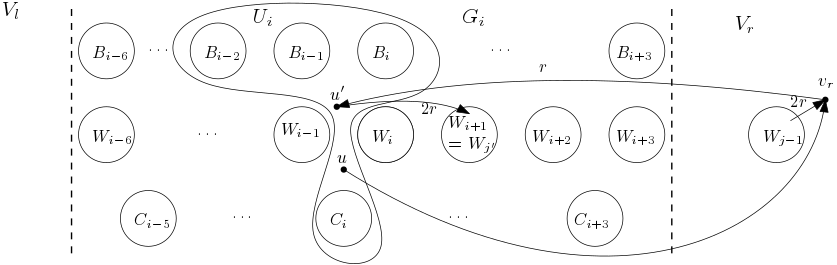 Figure 1
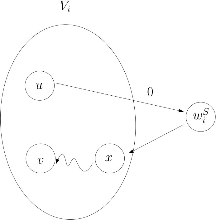 Figure 2
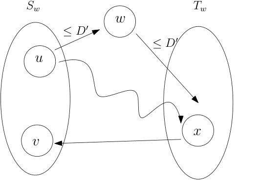 Figure 3
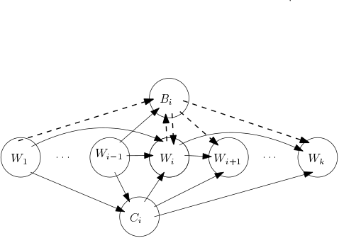 Figure 4
Peer Reviews
No public reviews on file for this paper yet. If you reviewed it on a platform where reviews are public (OpenReview, ICLR, NeurIPS, ICML), you can paste yours below so the community can read it here.
Videos
No videos yet. Explain this paper in a talk, walkthrough, or lecture? Add one.
Approximation Algorithms for Min-Distance Problems
Mina Dalirrooyfard, Virginia Vassilevska Williams, Nikhil Vyas,
Nicole Wein, Yinzhan Xu and Yuancheng Yu [email protected], [email protected], [email protected], [email protected], [email protected], [email protected], MIT EECS and CSAIL
Abstract
We study fundamental graph parameters such as the Diameter and Radius in directed graphs, when distances are measured using a somewhat unorthodox but natural measure: the distance between and is the minimum of the shortest path distances from to and from to . The center node in a graph under this measure can for instance represent the optimal location for a hospital to ensure the fastest medical care for everyone, as one can either go to the hospital, or a doctor can be sent to help.
By computing All-Pairs Shortest Paths, all pairwise distances and thus the parameters we study can be computed exactly in time for directed graphs on vertices, edges and nonnegative edge weights. Furthermore, this time bound is tight under the Strong Exponential Time Hypothesis [Roditty-Vassilevska W. STOC 2013] so it is natural to study how well these parameters can be approximated in time for constant . Abboud, Vassilevska Williams, and Wang [SODA 2016] gave a polynomial factor approximation for Diameter and Radius, as well as a constant factor approximation for both problems in the special case where the graph is a DAG. We greatly improve upon these bounds by providing the first constant factor approximations for Diameter, Radius and the related Eccentricities problem in general graphs. Additionally, we provide a hierarchy of algorithms for Diameter that gives a time/accuracy trade-off.
1 Introduction
The diameter, radius and eccentricities of a graph are fundamental parameters that have been extensively studied [13, 19, 12, 17, 3, 14, 11, 16, 5, 6, 25, 26, 9, 18, 23, 22, 10, 1, 7] (and many others). The eccentricity of a vertex is the largest distance between and any other vertex. The diameter is the maximum eccentricity of a vertex in the graph, thus measuring how far apart two nodes can be, and the radius is the minimum eccentricity, measuring the maximum distance to the most central node.
The distance between two vertices in an undirected graph is just the shortest path distance between them. For directed graphs, however, this notion of distance is no longer necessarily symmetric, and rather than being a distance between two nodes, it measures the distance in a given direction. Several related notions of pairwise distance that are symmetric have been studied. These include the roundtrip distance [15] which for two vertices and is just , the max-distance [2] which is , and the min-distance [2] which is .
Each of these notions of distance has a particular application. For instance, one would have to pay the roundtrip distance when going to the store and back. On the other hand, if one needs medical assistance, one could either go to the hospital, or have a physician come to the home — the time to receive care is then measured by the min-distance. Another example of min-distance is in symmetric-key encryption: any pair of parties can create a shared private key by using only one-way communication.
For each notion of distance, the diameter, radius and eccentricity parameters are well-defined. Given the shortest path distances for all vertices, the parameters for each distance measure can be computed in time in vertex graphs. The fastest known algorithms for All-Pairs Shortest Paths (APSP) [24, 20, 21] give the fastest known algorithms to compute these parameters exactly, running in time and , respectively on -edge, -vertex graphs. Furthermore, under the Strong Exponential Hypothesis, there is no time algorithm for Diameter in unweighted graphs (and thus also for any of these notions of Diameter and Eccentricities in directed graphs) [22]. For Radius, the same lower bound holds but under the “Hitting Set” conjecture [2].
As exact computation is expensive, it makes sense to resort to approximation algorithms. For the shortest path distance versions of Diameter, Eccentricities and Radius, there are several fast algorithms that achieve various small constant approximation ratios [22, 10, 8, 4]. For instance, for Diameter, a folklore linear time algorithm can achieve a -approximation, and an time111We use notation to hide polylogarithmic factors algorithm can achieve a -approximation [22, 10].
Many of these algorithms [22, 10, 4] work for any distance measure that satisfies the triangle inequality. Thus they work for the shortest paths distance, max-distance and roundtrip distance. The min-distance however does not satisfy the triangle inequality: e.g. you might have edges and , and thus the min-distance between and and between and are both , yet there may be no directed path between and in any direction, so that the min-distance between them may be .
This issue makes it much more difficult to design fast approximation algorithms for Min-Diameter, Min-Radius and Min-Eccentricities (the parameters of interest under the min-distance). The only known nontrivial algorithms are by Abboud et al. [2]. For Min-Diameter [2] gives a near-linear time -approximation algorithm if the input is a directed acyclic graph. For general graphs, the only nontrivial fast approximation algorithm is an time -approximation algorithm for any constant . (No constant factor approximation algorithm is known that runs significantly faster than just computing APSP.) For Min-Radius, [2] gives an time -approximation algorithm for directed acyclic graphs. For general graphs, they only achieve a very weak -approximation in near-linear time that checks if the Min-Radius is finite. There are no known approximation algorithms for Min-Eccentricities faster than just computing APSP.
1.1 Our Results
The main goal of our paper is to obtain new fast, time for some constant , algorithms for Min-Diameter, Min-Radius and Min-Eccentricities (thus beating the time of exact computation). We achieve this by developing powerful new techniques that can handle the complications that arise due to the fact that the min-distance does not satisfy the triangle inequality.
Our results are as follows. For Min-Diameter we achieve a hierarchy of algorithms trading off running time with approximation accuracy.
Theorem 1.1**.**
For any integer , there is an time randomized algorithm that, given a directed weighted graph with edge weights non-negative and polynomial in , can output an estimate such that with high probability, where is the min-diameter of .
When we set , we obtain an time -approximation algorithm, and when we set , we get an time -approximation.
Our tradeoff achieves the first constant factor approximation algorithms for Min-Diameter in general graphs that run in time for constant . Such a result was only known for directed acyclic graphs, whereas for general graphs the only known efficient algorithm could achieve an -approximation.
For Min-Radius, we also achieve the first constant factor approximation algorithm for general graphs running in time for some constant . Such a result was only known for directed acyclic graphs, whereas for general graphs the only known efficient algorithm could only check if the Min-Radius is finite.
Theorem 1.2**.**
For any constant with , there is an time randomized algorithm, that given a directed weighted graph with edge weights positive and polynomial in , can output an estimate such that with high probability, where is the min-radius of .
Finally, we obtain the first time (for constant ) constant factor approximation algorithms for the Min-Eccentricities of all vertices in a graph. For unweighted graphs we are able to obtain a close to approximation in time. For weighted graphs, our approximation factor grows to , while the running time is the same. Previously, the only algorithm to approximate the Min-Eccentricities computed them exactly via an APSP computation.
Theorem 1.3**.**
For any constant with , there is an time randomized algorithm, that given a directed weighted graph with weights positive and polynomial in , can output an estimate for every vertex such that with high probability, where is the min-eccentricity of vertex in .
Theorem 1.4**.**
For any constant with , there is an time randomized algorithm, that given a directed unweighted graph , can output an estimate for every vertex such that with high probability, where is the min-eccentricity of the vertex in .
1.2 Our Techniques
To obtain our results, we develop powerful new techniques which we outline below.
Partial search graphs.
The idea of partial search graphs is used in the algorithms of [2] for Min-Radius and Min-Diameter on DAGs. These algorithms use the following high-level framework: perform Dijkstra’s algorithm from some vertices and then perform a partial Dijkstra’s algorithm from every vertex. The partial search from a vertex is with respect to a carefully defined partial search graph . The crux of the analysis for the algorithms on DAGs is to argue that if the executions of Dijkstra’s algorithm on the full graph did not find a good estimate for the desired quantity (either min-diameter or min-radius), then the partial search from some vertex returns a good estimate of the min-eccentricity of , which in turn is a good estimate for the desired quantity. In DAGs it is natural to define the partial search graphs by considering a topological ordering of the vertices and letting each be some interval containing (though defining the exact intervals requires some work). For general graphs it is completely unclear how to even define such intervals since there is no natural notion of an ordering of the vertices, and thus figuring out what the ’s should be is nontrivial. Our approach to overcoming this hurdle is to carefully define a DAG-like structure in general graphs. Such a structure may be of independent interest.
Defining a DAG-like structure in general graphs.
It would be ideal to directly reduce the problem on general graphs to the problem on DAGs, however it is very unclear how to do this. Instead, we recognize that it suffices to define a DAG-like structure in general graphs. As a first step, we use the following idea. Suppose we have performed Dijkstra’s algorithm from a vertex . We let and we let 222’s with are added to either or as specified in the formal definition later. Then, we partially order the vertices so that the vertices in appear before and those in appear after . We note that this partial ordering is “DAG-like” because it is consistent with the topological ordering of a DAG; that is, if we apply this partition into and to a DAG then there trivially exists a topological ordering such that every vertex in appears before and every vertex in appears after . After partitioning into and , we recursively partition each set to create a more precise partial ordering. Importantly, we show that by recursively sampling vertices randomly, we can guarantee that our partitioning is approximately balanced which is crucial for the runtime analysis. The obtained partial ordering is the starting point for all of our algorithms.
Min-Diameter: graph augmentation.
The Min-Diameter algorithm on DAGs from [2] relies heavily on the following key property of DAGs. Consider a topological ordering and the graphs induced by the first and second halves of the ordering; which are defined with respect to the middle vertex in the ordering. For all pairs of vertices in the same half of the ordering, their min-distance in the graph induced by this half is the same as their min-distance in the full graph. As previously mentioned, if we sample a vertex , we can make sure that and are approximately balanced, so that we can think of and as corresponding to the first and second half of a DAG topological ordering, respectively. However it is unclear how to obtain a property of and analogous to the above key property of DAGs. In particular, the min-distance between a pair of vertices in the graph induced by could be wildly different from their min-distance in the full graph, since paths whose endpoints are in can contain vertices outside of . To overcome this hurdle, we augment the graph induced by and the graph induced by by carefully adding edges so that distances within these augmented graphs approximate distances in the original graph.
Min-Radius: refined DAG-like structure
Our Min-Radius algorithm is much more delicate than our Min-Diameter algorithm due to the fact that for Min-Radius we care about small distances instead of large distances. In particular, the graph augmentation idea from our Min-Diameter algorithm does not help for Min-Radius because although the augmentations do not distort large distances much, they heavily distort small distances. Furthermore, the previously mentioned DAG-like structure for general graphs does not suffice for Min-Radius. However we use it as a starting point to define a more refined DAG-like partial ordering. Most of our algorithm is concerned with precisely arranging vertices in this partial ordering. Specifically, we structure the partial ordering to satisfy roughly the following property: for every pair of vertices , such that appears before in the partial ordering, is large while is small.
1.3 Notation
Given a graph , and . Graphs are directed and have non-negative weights polynomial in unless otherwise specified. For any pair of vertices and , the distance from to is the length of the shortest directed path from to . When the context is not clear, we write to specify the graph . The min-distance between a pair of vertices and is . The min-diameter of a graph is . The min-radius of a graph is . For any vertex , the min-eccentricity of is . When the context is not clear, we say to specify the graph . Note that we do not use the min subscript to denote the min-eccentricity of a vertex. For an algorithm with input size we use with high probability to denote the probability for all constants . We say some quantity is to mean it is for some fixed constant . We use notation to hide polylogarithmic factors.
1.4 Organization
In Section 2 we give an overview of all of our algorithms, in Section 3 we describe a graph partitioning procedure that begins all of our algorithms, in Section 4 we describe our Min-Diameter algorithms, in Section 5 we describe our Min-Radius algorithm, and in Section 6 we describe our Min-Eccentricities algorithm.
2 Overview of Algorithms
We use the algorithms from [2] for Min-Diameter and Min-Radius on DAGs as inspiration. For each problem, we first outline the DAG algorithm and then provide intuition for how to apply these ideas to general graphs.
2.1 Min-Diameter
Algorithm for DAGs
We begin by outlining the time 2-approximation algorithm for Min-Diameter on DAGs from [2]. Consider a topological ordering of the vertices and perform Dijkstra’s algorithm from the middle vertex . Then recurse on the graphs induced by the vertices in the first half (before ) and in the second half (after ). A key observation in the analysis is that if the true endpoints and of the min-diameter fall on opposite sides of in the ordering, then the min-eccentricity of is a 2-approximation for the min-diameter . This is because if and and fall on opposite sides of in the ordering, then and so , a contradiction. So, suppose (without loss of generality) that and both fall before in the ordering. Since the graph is a DAG, every path between and only uses vertices before in the ordering. Thus, the min-distance between and in the graph induced by the first half of the graph is still .
Algorithm for general graphs
We now outline a precursor to our Min-Diameter algorithm for general graphs that mimics the algorithm for DAGs. This time algorithm does not achieve a constant approximation factor, however it provides intuition for our constant-factor approximation algorithms. We begin by performing Dijkstra’s algorithm from a vertex and constructing and as defined in the previous section. Analogously to the DAG algorithm if the true min-diameter endpoints and fall into different sets , then the min-eccentricity is a 2-approximation. This is because if , , and then and so , a contradiction. However, unlike the DAG algorithm, we cannot simply recurse independently on the graphs induced by and since the shortest path between a pair of vertices in may not be completely contained in (and analogously for ).
To overcome this hurdle, before recursing we first augment the graphs induced by and by carefully adding edges so that distances within these augmented graphs approximate distances in the original graph. Specifically, for every vertex , we add the directed edge with weight 0 and the directed edge with weight . This choice of edges allows us to argue that the distances within the augmented graphs are approximations of the distances in up to an additive error of . Then, by returning the maximum of and the min-diameter estimates from recursing on the augmented graphs, we get an approximation guarantee, which turns out to be a logarithmic factor. Intuitively, the approximation factor is not constant because the recursion causes the distance distortion to compound at each level of recursion.
To reduce the approximation factor to a constant, we would like to decrease the number of recursion levels. To achieve this, we initially partition the graph into more than just two parts and , by sampling more vertices. For our time 3-approximation, we perform a full Dijkstra’s algorithm from vertices to define an ordered partition of the vertices into parts of vertices each. Then we apply the above idea of adding weighted edges within each part, however we must refine the definition of the graph augmentation to take into account all of the vertices we initially perform Dijkstra’s algorithm from, instead of just . Finally we use brute force (without recursion) on each part in the partition by running an exact all-pairs shortest paths algorithm.
To achieve our time-accuracy trade-off algorithm, we carefully combine ideas from the logarithmic factor approximation and the 3-approximation algorithms. Specifically, we initially perform Dijkstra’s algorithm from fewer than vertices to define an ordered partition with larger parts than in the 3-approximation. Then we augment the graph induced by each part and carry out a constant number of recursion levels to further partition the graph before applying brute-force.
2.2 Min-Radius
Algorithm for DAGs
We begin by outlining the time 3-approximation algorithm for Min-Radius on DAGs from [2], which is very different from and more involved than the Min-Diameter algorithm on DAGs. We begin by considering a topological ordering of the vertices and performing Dijkstra’s algorithm from a set of evenly spaced vertices including the first and last vertex. If a vertex has min-eccentricity at most twice the true min-radius then we have obtained a 2-approximation. (We do not know in advance but we repeatedly run the algorithm with different values of to perform a binary search on .)
Otherwise, we will define intervals in the ordering such that the min-center cannot be contained in any of these intervals. A key observation is that if there is a pair of vertices such that appears before in the topological ordering and , then the min-center cannot fall between and in the topological ordering. This is because if it did, then and , so , a contradiction. We define the intervals that cannot contain as follows: for all we let be the first vertex in the ordering such that (if it exists, otherwise ) and define to be the last vertex in the ordering such that (if it exists, otherwise ). Then, the key observation implies that cannot fall in the interval in the ordering. Now, we have a set of possibly overlapping intervals that cannot contain . We take the union of these intervals to get a set of disjoint intervals that cannot contain .
Every vertex that does not appear in such an interval, falls between two consecutive intervals and . We define the partial search graph of to be the graph induced by the set of vertices in or or between and . After performing the partial searches, the algorithm returns 3 times the minimum min-radius of all partial search graph. Next we give the idea of the analysis, which demystifies the factor of 3 in the returned value.
We claim that if the min-eccentricity of a vertex with respect to its partial search graph is at most , then its min-eccentricity with respect to the full graph is at most , and the min-eccentricity of the true min-center with respect to its partial search graph is at most (because for any path in a DAG whose starting and ending points are in a certain interval, every vertex in the path is in that interval). Thus, assuming the claim, is a 3-approximation for the min-radius. We now outline the proof of the claim. Let be the min-center with the minimum min-radius of all partial search graphs. Let such that is the first vertex (in the topological order) of , then and . Furthermore, by the definition of , all vertices that appear before the beginning of the interval have distance at most to , and thus distance at most to . A symmetric argument holds for vertices that appear after the end of the interval . Hence the min-eccentricity of with respect to the full graph is at most .
This algorithm runs in time because the vertices of are evenly spaced so there are no more than vertices between each pair of consecutive intervals. This implies that in the partial searches, each edge is only scanned times. (Furthermore, repeatedly running the algorithm to binary search for adds a logarithmic factor to the runtime.)
Algorithm for general graphs
We now give a high-level outline of our time 3-approximation algorithm for Min-Radius. This algorithm is much more delicate than our Min-Diameter algorithm, hence more of the details are deferred to the full description. We begin by running Dijkstra’s algorithm from a set of randomly sampled vertices to recursively partition the vertices into and as outlined in Section 1.2. This defines an initial DAG-like structure, however our analysis requires constructing a much more refined DAG-like structure.
Perhaps counter-intuitively, it makes sense to place vertices that are far from each other in the graph close to each other in the DAG-like structure. The reason for this is illuminated by the Min-Radius algorithm on DAGs, in which we find pairs of vertices that are far from each other and apply the key observation that the min-center cannot be between and in the topological ordering. Intuitively, it is as if we collapse the interval between and in the DAG since we do not have to search within this interval for the min-center. An analogous key observation is true for general graphs: if there is a pair of vertices with , then either or . This is because if , then and so , a contradiction; the last case is symmetric. In our algorithm for general graphs, we ensure that far vertices are near each other in the DAG-like structure by doing the following: we let the far graph be an undirected graph on with an edge between and if . All vertices in that are in the same connected component in will be grouped in the DAG-like structure. We let be the set of vertices in that are in the connected component of .
To construct the DAG-like structure, we show that precisely chosen groups of s can be merged to create supercomponents, which constitute a DAG-like structure in the following sense: there is an ordering of supercomponents such that for every pair of vertices where the supercomponent containing appears before that containing , is small and is large. Specifically, we define the close graph whose vertex set is the set of s. We add a directed edge between a pair of vertices in if there exists a short path (length ) between the corresponding s. Then we merge all s that appear in the same strongly connected component of into a supercomponent. This contraction of strongly connected components of results in a DAG, which defines the ordering of the supercomponents.
Now that we have arranged the vertices in into a DAG-like structure, we would like to fit every vertex in the graph into this structure. Based on the precise way that we have defined the supercomponents, we can use an intricate argument to show roughly the following property: for every vertex there exists an such that for every vertex in the first supercomponents, is small and for every vertex in the remaining supercomponents, is small.
After fitting every vertex into the refined DAG-like ordering, we can define each partial search graph to be an interval in the ordering that is large enough to contain several supercomponents. In the algorithm for DAGs, there were two important properties of the partial search graphs: (1) the min-eccentricity of the true min-center with respect to its partial search graph is at most , and (2) if the min-eccentricity of a vertex with respect to its partial search graph is at most then its min-eccentricity with respect to the full graph is at most . We show that due to the precise structure of the supercomponents, refinements of properties (1) and (2) are also true for general graphs.
Intuitively, property (1) is roughly true because for every pair of vertices such that ’s supercomponent appears before ’s in the ordering, , since otherwise this pair of supercomponents would be in the same strongly connected component of and would have been merged into a single supercomponent. This implies that paths of length at most to or from the min-center cannot stray beyond its partial search graph. Intuitively, property (2) is roughly true because for every pair of vertices such that ’s supercomponents appears before ’s in the ordering, because otherwise, and would be in the same component of and thus be in the same supercomponent. Thus, like the argument for DAGs, for all , all vertices that appear before ’s partial search graph have distance at most to each supercomponent in , and thus distance at most to . A symmetric argument holds for vertices after in the ordering.
2.3 Min-Eccentricities
Our Min-Eccentricities algorithm is a modification of our Min-Radius algorithm. In our Min-Radius algorithm, we identify a vertex whose min-eccentricity is at most about , where is the true min-radius. In our Min-Eccentricities algorithm, we show that with some extra bookkeeping, the algorithm can identify all vertices with min-eccentricity at most about for any . We run the algorithm repeatedly, increasing by a factor of at each execution until we have estimated the min-eccentricity of every vertex.
The major modification of the Min-Radius algorithm here is that if one of the vertices that we run Dijkstra from has min-eccentricity at most , we cannot stop running the algorithm, as we can in the Min-Radius algorithm. Instead, we use this vertex as a tool to find vertices with min-eccentricity at most .
3 Preliminary Graph Partitioning
In this section we describe a graph partitioning procedure we use as a first step in our Min-Diameter, Min-Radius, and Min-Eccentricities algorithms. The goal of this partitioning is to define a DAG-like structure in general directed graphs.
Definition 3.1**.**
Assign each vertex a unique ID from . For each vertex , let . Let .
The runtime of our algorithms relies on whether the partition into and is balanced. Using the observation that if , then , the following lemma shows that for most vertices, the partition is indeed approximately balanced.
Lemma 3.1**.**
For any graph on vertices there are more than vertices such that .
More generally, for any , there are more than vertices such that .
Proof.
Since the first statement is a special case of the second statement with , we prove the more general statement. Let . Let be a matrix indexed by the vertices in where if , if , and for . Note that is skew-symmetric, i.e., for all . For any , let be the submatrix consisting of the columns indexed by , and let the submatrix of consisting of its rows indexed by .
Suppose for contradiction there is a set of vertices such that . Then contains at least ones.
The submatrix is also skew-symmetric, so at most half of its entries are ones, i.e., contains at most ones. Letting , we see that has entries, and hence at most ones. In total, contains at most ones, contradiction.
Therefore the number of vertices such that is less than , and symmetrically the number of vertices such that is less than . Hence more than half of the vertices have that .
Next, we describe how we use Lemma 3.1 to recursively construct a balanced partition of the vertices into a given number of of sets.
Lemma 3.2**.**
Given a graph with vertices and a constant , in time we can partition into disjoint sets , ,…,, where , such that with high probability:
for all , ; 2. 2.
for all , there exists a vertex such that either ,, or ,; 3. 3.
for all , let , then for some .
Proof.
We begin with and we will iteratively populate with vertices. We let and for all when we add the vertex to , we will construct from by partitioning the largest set in into two parts. After adding vertices to we will have constructed .
For all , let be the largest and smallest sets in , respectively.
We describe how to construct and inductively. Suppose and we have constructed . By Lemma 3.1, if we randomly sample vertices from , with probability at least we will sample a vertex such that and differ by a factor of at most . We add to and let .
By union bound over the partitionings, with probability at least , every partitioning produces two sets that differ in size by a factor of at most 8.
We prove property 1 by induction on . Specifically, we will show that for all , . This implies that , and property 1 follows. Lemma 3.1 implies that . Assume inductively that . Since no subset grows in size, and . If , then . Otherwise, , which implies that is one of the two sets obtained by partitioning . In this case by Lemma 3.1. Hence , completing the induction.
Property 2 follows from the partitioning procedure: for any , if for all , or then would never have been partitioned.
Property 3 also follows from the partitioning procedure: observe that for all and all , or , so is never partitioned and thus for some .
Since we sample vertices and for all finding takes time, the runtime is .
4 Min-Diameter Algorithm
Throughout this section, let be the min-diameter, and let the endpoints of the min-diameter. In this section we prove the time/accuracy trade-off theorem for Min-Diameter.
Theorem 4.1**.**
For any integer , there is an time randomized algorithm that, given a directed weighted graph with edge weights non-negative and polynomial in , can output an estimate such that with high probability, where is the min-diameter of .
We first prove a special case of Theorem 4.1 where .
4.1 An time 3-approximation
Theorem 4.2**.**
(Theorem 4.1* with ) There is an time randomized algorithm, that given a directed weighted graph with edge weights non-negative and polynomial in , can output an estimate such that with high probability, where is the min-diameter of .*
4.1.1 Algorithm Description
Applying Lemma 3.2 with we obtain a partition of the vertices into .
We perform Dijkstra’s algorithm from every vertex in and define . We will later show that is a good approximation of the Min-Diameter when and are not in the same vertex set .
For every , define , and . Then, for every , we construct two graphs and . The first graph contains all vertices of and an additional node . It has the following edges:
For every directed edge such that , add this edge to . 2. 2.
Add a directed edge from to every , with weight , and a directed edge from every to with weight [math].
The second graph is symmetric to . It contains all vertices in and an additional node . It has the following edges:
For every directed edge such that , add this edge to . 2. 2.
Add a directed edge from every to , with weight , and add a directed edge from to every with weight [math].
For all , we run an exact all-pairs shortest paths algorithm on and . This allows us to compute for all and all the quantity , which we denote by .
We choose the larger between and as our final estimate for the min-diameter.
4.1.2 Analysis
The following lemma will be used to show that is a good estimate for the min-diameter if and happen to fall into different sets
Lemma 4.1**.**
For all vertices , if either , , or , , then .
Proof.
We only consider the case when and as the other case is symmetric. By way of contradiction, assume that , then we have and . Since , ; similarly, since , . Therefore, by the triangle inequality, , a contradiction.
The next two lemmas are used for the case where and fall into the same set .
Lemma 4.2**.**
*For every , and every pair of vertices , ; that is,
.*
Proof.
Take any shortest path in the original graph from to . If this path does not leave , then this path also exists in and , and thus the inequality is true.
It remains to prove for the case when the shortest path in the original graph leaves . Let be any vertex on a shortest path. By Lemma 3.2, property 2, there exists such that and , or and . We first assume and as shown in Figure 1, and the other case is symmetric.
Since is on the shortest path from to , we have . Also, we have , by definition of . Therefore,
[TABLE]
Now consider the path in . The first part costs [math], because there is an edge from to with weight [math]; the second part costs at most . If , then ; otherwise, , where the last step is Equation 1.
When , and , we have a symmetric argument: . Consider the path in . The second part costs [math], because there is an edge from to with weight [math]; the first part costs at most . If , then ; otherwise, .
Lemma 4.3**.**
For every , and every pair of vertices , ; that is, and .
Proof.
We only provide full proof for . The inequality for can be proved by a symmetrical argument. If the shortest path from to in does not contain , then this path also exists in the original graph , and thus the inequality is true.
Otherwise, the shortest path from to in contains , as shown in Figure 2. All edges on the shortest path from to exist in the original graph except for the first edge from to some node , since a shortest path cannot use the vertex more than once. That is, .
By the definition of and the edges incident to it, there exists a such that . Thus, we have
[TABLE]
We are now ready to prove our approximation ratio guarantee: . Clearly because is the min-eccentricity of a vertex. By Lemma 4.2 . Therefore, we never over estimate the Min-Diameter.
If or , then since we run Dijkstra from all vertices in we have . So assuming that , we have two cases.
Case 1: and are not in the same vertex set . By Lemma 3.2, property 2, there exists such that one of and is in and the other is in , so by Lemma 4.1, . Since , we have .
Case 2: and are in the same vertex set for some . By Lemma 4.3, . Since , we get a -approximation.
Runtime analysis
It takes time to perform the partitioning from Lemma 3.2 and to perform Dijkstra’s algorithm from all since .
For all , the number of vertices in is with high probability by property 1 of Lemma 3.2 and the number of edges is where is the number of edges in the graph induced by . Hence we can run an all-pairs shortest paths algorithm on in time . Summing over all gives us . The same analysis also works for .
4.2 Time/accuracy trade-off algorithm
4.2.1 Algorithm Description
We begin by briefly outlining the differences between our trade-off algorithm and our time algorithm. For our trade-off algorithm, instead of applying Lemma 3.2 to sample vertices, we will apply Lemma 3.2 with a smaller value of to save time. This results in a smaller set and larger sets . In our time algorithm, we had time to apply brute force (i.e. run all-pairs shortest paths) on the graphs and , however in our trade-off algorithm we do not. Instead, we apply recursion. Simply constructing and and recursing on both of them does not suffice because each recursive call only returns the min-diameter, whereas we require knowing all distances. To overcome this issue, instead of constructing and separately, we construct a graph that combines these two graphs. Then, we show that it suffices to recurse on to compute only its min-diameter rather than all distances.
The algorithm is as follows. We apply Lemma 3.2 with to partition the vertices into . We perform Dijkstra’s algorithm from every vertex in and define . For every , we define , and . For every , we construct the graph as follows. The vertex set of is all vertices and two additional vertices and . It contains the following edges:
For every directed edge such that , add this edge to . 2. 2.
Add a directed edge from to every , with weight , and add a directed edge from every to with weight [math]. 3. 3.
Add a directed edge from every to , with weight , and add a directed edge from to every with weight [math].
For all , we recursively compute a -approximation for the Min-Diameter of by calling the algorithm for . We use the algorithm from the previous section as the base case.
We choose the larger between and the maximum approximated Min-Diameter over all as our final estimate.
4.2.2 Analysis
Before proving the main theorem for Min-Diameter, we need to prove two lemmas for , which are analogous to Lemma 4.2 and Lemma 4.3.
Lemma 4.4**.**
For every , and every pair of vertices , .
Proof.
Since and , we have and . Then by Lemma 4.2, we have .
Lemma 4.5**.**
For every , and every pair of vertices , .
Proof.
Consider the shortest path from to in . If this path does not contain both and , then this path exists in or , and thus we can directly apply Lemma 4.3 to get , or .
Otherwise, the shortest path from to contain both and . Such path can only be one of the following two forms:
- •
for some vertex . The first half is contained in , so we can apply Lemma 4.3 to get ; similarly, the second half is contained in so . In total, .
- •
for some vertex . We can similarly split this path to two halves, and apply the same analysis as the previous case to get .
We are now ready to prove our approximation ratio guarantee: . We prove the result inductively. When , it is exactly Theorem 4.2. Now assume it is true for , and we will prove it for .
Clearly because is the min-eccentricity of a vertex. By induction, the -approximation for the min-diameter of never exceeds the true min-diameter of . Then by Lemma 4.4, the min-diameter of does not exceed the min-diameter of . Therefore, we never over estimate the min-diameter.
If or , then since we run Dijkstra from all vertices in we have . So assuming that , we have two cases.
Case 1: and are not in the same vertex set . By Lemma 3.2, property 2, there exists such that one of and is in and the other is in , so by Lemma 4.1, . Since , we have .
Case 2: and are in the same vertex set for some . If , is already a good approximation. So assume . By Lemma 4.5, . Since we calculate a -approximation of ’s min diameter, our estimate is at least
[TABLE]
Runtime analysis
It takes time to perform the partitioning from Lemma 3.2 and to perform Dijkstra’s algorithm from all since . For all , the number of vertices in is with high probability by Lemma 3.2, property 1, and the number of edges is where is the number of edges in the graph induced by . By induction, it takes time to compute a -approximation of Min-Diameter of for each . Summing over all gives us .
Note that we apply Lemma 3.2 at most times in the recursion and this the only randomization so the whole algorithm works with high probability.
5 Min-Radius Algorithm
Theorem 5.1**.**
For any constant with , there is an time randomized algorithm that, given a directed weighted graph with weights positive and polynomial in , can output an estimate such that with high probability, where is the min-radius of the .
Proof.
We fix a value and our algorithm either certifies that or . Then by a binary search argument we get a -approximation as follows. Let . Starting from , we run the algorithm and increase for each run. If the output of the algorithm is that , then we stop. Otherwise (if ), we run the algorithm with the new value . This contributes a multiplicative factor of to the total runtime. Suppose that for some value of we have . So from the previous run of the algorithm, we know that . Letting , we have , which means that is a -approximation. Now we present the algorithm.
Algorithm Step 1: Preliminaries
Let be the min-center (which is unknown). First we remove all the edges with weight more than , because if , this removal does not change the min-radius. Then we sample a set of vertices according to Lemma 3.2. For every vertex , we run Dijkstra’s algorithm from and to to obtain the min-distance between and all other vertices. If there exists a vertex with , we have certified that so we are done.
Algorithm Step 2: Constructing the “far graph”
Now we can assume that for each , . We say that a pair of vertices is far if their min-distance is more than , and let the far graph be an undirected unweighted graph on defined as follows: for each and , is an undirected edge if and are far. We partition based on the connected components of . Specifically, for all define to be the connected component of which contains at least one vertex in . Let , note that is non-empty.
Analysis Step 2
Remember that we defined and .
By constructing , we prune the set of candidate min-centers, as specified in the following lemma.
Lemma 5.1**.**
If , then for any either or .
Proof.
First note that we have . We know that as . By way of contradiction, assume that there are two vertices such that . Consider a path in from to . There must be a pair of adjacent vertices on the path such that . Then, by definition, and are far (with respect to the original graph ). Since , we have and , so by the triangle inequality . Thus and are not far, a contradiction.
Algorithm Step 3: Defining a DAG-like structure
a) Constructing the “close graph”
The purpose of constructing the close graph is that it allows us to either perform Dijkstra’s algorithm from some additional vertices and obtain a good estimate (see step b), or “merge” some connected components of the far graph to further prune the set of vertices that could be the min-center (see step c). The close graph is an unweighted directed graph with one vertex for each . For all and , let be an edge in if for some and some , .
b) Additional Dijkstra
We now perform Dijkstra’s algorithm from some additional vertices, which are carefully chosen so that either we find a vertex with small min-eccentricity and are done in this step, or we can define a DAG-like structure in the graph (step c). We compute the strongly connected components (SCCs) of . For each SCC , find with such that is strongly connected; it is simple to show that such an exists and we include the proof in the appendix for completeness (Lemma A.2). Let . Note that every edge corresponds to a path of length at most in the original graph . For each , find an ordered set of at most 9 vertices on that divide into subpaths of length at most ; it is simple to show that such a exists and we include the proof in the appendix for completeness (Lemma A.1). We run Dijkstra’s algorithm from every vertex in and if we find a vertex with then we are done.
c) Constructing the DAG of “supercomponents”
Let be the DAG created by contracting every strongly connected component of into a single vertex. That is, there is an edge from to in if the strongly connected component is reachable from the strongly connected component . Let be the number of vertices in ; we number the vertices in from 1 to according to a topological ordering. For each , we merge the set of ’s represented by vertex in into a supercomponent . Formally, if we define to be the connected component of that contains , a vertex is in supercomponent if is in the strongly connected component of represented by vertex .
d) Fitting the remaining vertices into the DAG structure
In the previous step, we defined a DAG-like structure on the vertices in . Now we place the rest of the vertices into this structure. We partition the rest of the vertices based on whether they could potentially be the min-center. We define the vertex sets and next and in the analysis we prove that (among other properties of and ). We will use the following notation: for any distance , let and let . Remember that for any set of vertices, we defined , and .
- •
For , let if for all , and for all , . Let .
- •
For , let if and is the largest integer for which . Let if there is no such and . Let .
Analysis Step 3
Figure 3 shows a summary of the structure of the graph which we will describe in the following observations and lemmas.
We first observe two important properties of supercomponents:
Observation 5.1**.**
For every pair of vertices and with , .
This is true because if , then there is an edge from to in , so there is an edge from to in . Since , this contradicts the topological ordering of .
Observation 5.2**.**
For every pair of vertices and with , and .
This is true because and are in different ’s since and are collections of disjoint sets of ’s. So and are not far i.e. and by Observation 5.1 we know that , so it must be that . Since this is true for all vertices , we have . Similarly, .
We now prove a refinement of Lemma 5.1 where we consider supercomponents instead of far graph components. This further prunes the vertices that could potentially be the min-center.
Lemma 5.2**.**
If , then for each , either or .
Proof.
Fix and suppose by way of contradiction that there are nodes such that . By Lemma 5.1, and must be in different ’s say and .
Recall that by the definition of a supercomponent, and are in the same strongly connected component of . So there is a path from to in such that all of its edges are in . By Lemma 5.1 Since , we have that . So there are two consecutive nodes and on (in that order) such that .
Recall that each edge corresponds to a path of length at most in the original graph. Let be the edge and consider and , where is the set of vertices that divides into subpaths of length at most . Since the endpoints of are in and respectively, there exists a pair of vertices consecutive in (in that order) such that . We note that .
Now we claim that . This is because and . Consider an arbitrary vertex . Either or . If then . If , then . In this case, the algorithm would have stopped after step 3b.
We now prove that , which further prunes the vertices that could potentially be the min-center.
Lemma 5.3**.**
If , then .
Proof.
By Lemma 5.2, either or . Since is the min-center and , if then , and similarly if then . We claim that for each , , which completes the proof. Suppose otherwise and let and be such that and there is a vertex . Then for every vertex and , and , so . This contradicts Observation 5.1.
Now we prove that the vertices in fit into the DAG structure in a similar but weaker sense than the vertices in :
Lemma 5.4**.**
Consider a node . Then for all except for at most two values, we have . And for all except for at most two values, we have .
Proof.
We first observe that there is at most one such that is far from some vertex in . This is because if were far from two vertices in different supercomponents, then would contain the edges and making and in the same connected component of , and thus in the same supercomponent. We fix and consider two cases:
Case 1: Suppose by way of contradiction that for some node for some , we have . We know that , since by definition of , we have . Let be an arbitrary node, then , a contradiction to Observation 5.1.
Case 2: Now suppose that for some node for some , we have . We will show that and ; that is, for all , we have that . If there is some node such that , then , a contradiction to Observation 5.1. Assume that there is no such i.e. for all . Then for every node , either and are far or . If for all , , then , which cannot happen since by the definition of , is the biggest integer that . Thus, is far from some vertex in so we have that . If , then by definition of there is some vertex such that . So , a contradiction to Observation 5.1. So it must be that . So for all , we have that .
We have observed stronger properties than Lemma 5.4 for vertices (Observation 5.2) and (by definition), so we have the following corollary.
Corollary 5.1**.**
Lemma 5.4 is true for all . Moreover, for such ’s, we have .
Algorithm Step 4: Partial search
From each of the potential min-centers, we will run Dijkstra’s algorithm on a small subgraph of . For each , let be the subgraph of induced by . Define to be the set of nodes such that is within min-distance from all vertices in (we know this set of nodes because we have already run Dijkstra’s algorithm from and to every vertex in ). For every vertex in , run Dijkstra’s algorithm from with respect to the graph . If is within min-distance from all nodes in , we will show that . If there is no such , we will show that .
Analysis Step 4
The following two claims prove that our algorithm either certifies that or .
Claim 1**.**
For some , if and , then for all , the min-distance between and with respect to is at most .
Claim 2**.**
If a vertex is within min-distance from all vertices in with respect to the graph , then .
Proof of Claim 1.
We will prove something slightly stronger: for all any shortest path in between two nodes that has length at most is completely contained in .
By way of contradiction, suppose that the shortest path from to is not completely in . Define and to be sets of nodes on the right and left of respectively, i.e. and .
First suppose that contains some node . There is some such that . So by Corollary 5.1, . Furthermore, Corollary 5.1 implies that there is some such that . Pick and . We have that . Since , this contradicts Observation 5.1. This case is shown in Figure 4.
Now suppose that contains some node in . The argument in this case is symmetric to the previous case. Since , there is some such that , and hence by Corollary 5.1, . Furthermore, Corollary 5.1 implies that there is at least one value such that . Pick and . We have that . Since , this contradicts Observation 5.1.
Proof of Claim 2.
We show that for any node we have . We have cases:
Case 1: : From the definition of , we know that has min-distance at most to all vertices in .
Case 2: for some . If , then so we know that . If , then pick some vertex . By the definition of and we know that . Similarly, if , pick some vertex . Then .
Case 3: for some . If , then since we know that . So first suppose that . Then by Lemma 5.4, there is at least one , such that . Pick some node . So by the definition of we have that . Now suppose that . Then by definition of we know that . Pick some vertex . Since and by the definition of , we have that
Runtime analysis
We analyze the running time of each step.
Step 1, preliminaries: . This is because each Dijkstra in Step 1 takes time and .
Step 2, constructing the “far graph”: . Each edge in the far graph has at least one endpoint in , and so the construction of the far graph takes time. Note that the existence of each edge in the far graph was determined in Step 1.
Step 3, defining a DAG-like structure:
**a, constructing the “close graph”: ** . This is because the connected components of the far graph can be determined in time since it has that many edges. The number of components containing a node in are not more than , and so the close graph which is on at most nodes can be constructed in time .
b, additional Dijkstra: . This is because by Lemma A.2, the number of vertices we run Dijkstra from in SCC of the close graph is at most . Since the number of vertices in close graph is at most , we run Dijkstra from at most vertices. Also running the algorithm of Lemma A.2 takes for each SCC , which takes time in total.
c, constructing the DAG of “supercomponents”: . This is because has at most vertices, so obtaining the DAG ordering of takes at most time.
d, fitting the remaining vertices into the DAG structure: . For each vertex in , it takes time to see which set it belongs to, since it only depends on its distances to and from the vertices in .
Step 4, partial search: . The Dijkstras ran in take time, where is the number of edges with at least one endpoint in . By Lemma 3.2, property 3, with high probability . We know that and so the running time of this step is . Now since each node is in at most s, we have that each edge is also in at most s, and hence .
So overall the algorithm runs in time.
6 Min-Eccentricities Algorithm
The min-eccentricities algorithm is similar to the min-radius algorithm. Below we will describe the modifications.
Theorem 6.1**.**
For any constant with , there is an time randomized algorithm, that given a directed weighted graph with weights positive and polynomial in , can output an estimate for every vertex such that with high probability, where is the min-eccentricity of the vertex in .
Proof.
We fix a value and our algorithm certifies for each that either or with high probability. Starting from , we will run the algorithm and increase for each run. We will call the vertices for which we have certified for earlier values of as marked. Let . Starting from , we run the algorithm. If the output of the algorithm is that and was unmarked, then we will mark and set . Then, we run the algorithm with the new value . Since for all , this contributes a multiplicative factor of to the total runtime. Suppose that for some value of and for some vertex we have and was unmarked. From the previous run of the algorithm, we know that . Then for , we have and , which means that is a -approximation of . After running the whole algorithm for this value of we will also mark all such vertices . Now we present the algorithm.
Throughout the algorithm behaves analogously to in the min-radius algorithm. Whenever we say that a certain part of the algorithm is the same we mean that it is same after replacing by . Note that any vertex with satisfies the property that its min-distance to any vertex is at most . This is analogous to the center vertex in the Min-Radius algorithm using .
Algorithm Step 1: Preliminaries
First we remove all the edges with weight more than , because if for a vertex with , this removal does not change the min-eccentricity of . Then we sample a set of vertices according to Lemma 3.2. For every vertex , we run Dijkstra’s algorithm from and to to obtain the min-distance between and all other vertices. This means we know for all and in particular we know if or . We use the vertices in with min-eccentricity less than to detect vertices with min-eccentricity less than in the graph.
Algorithm Step 2: Constructing the “far graph”
The far graph and the ’s are defined the same way as in the min-radius algorithm.
Analysis Step 2
The purpose of constructing is to prune the set of vertices that could potentially have low min-eccentricity. Next we state a modified Lemma 5.1.
Lemma 6.1** (Modification of Lemma 5.1).**
If for a vertex , , then for any , either or .
Proof.
For note that and hence we know and have certified either or . For the other vertices the proof is analogous to that of Lemma 5.1
Algorithm Step 3: Defining a DAG-like structure
a) Constructing the “close graph”
The purpose of constructing the close graph is that it allows us to perform Dijkstra’s algorithm from some additional vertices and certify some vertices as having min-eccentricities . Then we “merge” some connected components of the far graph to further prune the set of vertices that could be having small min-eccentricities (see step c). is defined as in the min-radius algorithm.
b) Additional Dijkstra
This step of the algorithm diverges from the min-radius algorithm at the end, and hence we state it in full detail. Similar to the min-radius algorithm, we perform Dijkstra’s algorithm from some additional vertices, which are chosen so that we detect more vertices with low min-eccentricity and at the end define a DAG-like structure (step c). Recall that we compute the strongly connected components (SCCs) of . For each SCC , find with such that is strongly connected (where the existence of is shown in Lemma A.2). Let . Recall that every edge corresponds to a path of length at most in the original graph . For each , find an ordered set of at most 9 vertices on that divide into sections of length at most (see Lemma A.1). For each , we run Dijkstra’s algorithm from and to every vertex in . This means we know for all ; and in particular we know whether or . Now here is the new part of the algorithm in this step: For every consecutive pair of vertices in over all with we certify for all that .
c) Constructing the DAG of “supercomponents”
The graphs , ’s and the “supercomponents” are defined as in the min-radius algorithm.
d) Fitting the remaining vertices into the DAG structure
In the previous step, we defined a DAG-like structure on the vertices of . Now we place the rest of the vertices into this structure. We partition the rest of the vertices based on whether they haven’t been certified to have eccentricity and could potentially have small eccentricity. Vertex sets and are defined as in the min-radius algorithm. In the analysis we prove that all vertices which haven’t been certified to have eccentricity and could potentially have small eccentricity must be in , among other properties of and .
Analysis Step 3
First note that one major difference of this algorithm and the min-radius algorithm is in part b; in the min-radius algorithm we stop whenever we find a good approximate center among the vertices in s, but here we can only upper bound the eccentricity of some vertices by if we find vertices with eccentricity among s.
We first show that if for some vertex and for some consecutive pair of vertices in such that and , then . This is derived by Lemma 6.2 which we state bellow, by the following substitution: let , and .
Lemma 6.2**.**
Consider vertices such that , and then .
Proof.
Consider a vertex , as either or . If then . Otherwise then . In both cases .
Now we observe an important property of supercomponents with an analogous proof to that of Observation 5.1.
Observation 6.1** (Modification of Observation 5.1).**
For every pair of vertices in and with , .
We now prove a modification of Lemma 5.2. This further prunes the vertices that could potentially have small eccentricity.
Lemma 6.3** (Modification of Lemma 5.2).**
If for a vertex , and we haven’t yet certified then for each , either or .
Proof.
Fix and suppose by way of contradiction that there are nodes such that and . By Lemma 6.1, and must be in different ’s say and .
Recall that by the definition of a supercomponent, and are in the same strongly connected component of . So there is a path from to in such that all of its edges are in . By Lemma 6.1 since , we have that . So there are two consecutive nodes and on (in that order) such that .
Recall that an edge corresponds to a path of length at most in the original graph. Let be the edge and consider and . Since the endpoints of are in and respectively, there exists a pair of vertices consecutive in (in that order) such that . We note that .
Recall that we assumed that Note as well that and . Then, using Lemma 6.2 with , we get that . A symmetric argument holds for , giving . In this case, the algorithm would have already marked in step 3b as it is in the intersection of .
We now prove that for vertices which have small min-eccentricity and have not been certified as such, . The proof is analogous to that of Lemma 5.3.
Lemma 6.4** (Modification of Lemma 5.3).**
If for a vertex , and we haven’t yet certified then .
Now we prove that the vertices in fit into the DAG structure in a similar but weaker sense than the vertices in . The proofs are analogous to those of Lemma 5.4 and Corollary 5.1.
Lemma 6.5** (Modification of Lemma 5.4).**
Consider a node . Then for all except for at most two values, we have . And for all except for at most two values, we have .
Corollary 6.1** (Modification of Corollary 5.1).**
Lemma 6.5 is true for all . Moreover for all , we have .
Algorithm Step 4: Partial search
From each of the potential vertices with small min-eccentricity in , we will run Dijkstra’s algorithm on a small subgraph of . and are defined as in the min-radius algorithm. Define to be the set of nodes such that is within min-distance from all vertices in (we know this set of nodes because we have already run Dijkstra’s algorithm from and to every vertex in ). From each node run Dijkstra’s algorithm from and to with respect to the graph . If is within min-distance from all nodes in , we will show that this certifies that and otherwise .
Analysis Step 4
The following two claims prove that our algorithm for vertices either certifies that or . The proofs are analogous to those of Claim 1 and Claim 2.
Claim 3** (Modification of Claim 1).**
If and , then for all , the min-distance between and with respect to is at most .
Claim 4** (Modification of Claim 2).**
If a vertex is within min-distance from all vertices in in , then .
For all the vertices for which we haven’t certified either or we know that and can certify that.
The runtime is with analogous runtime analysis to that of the min-radius algorithm.
6.1 -approximation for unweighted graphs
In this part we show that given an unweighted graph, by a slight modification of the min-eccentricity algorithm in Theorem 6.1, we are able to improve the approximation factor of the min-eccentricity problem to match that of the min-radius problem, namely we present a -approximation algorithm for every .
Theorem 6.2**.**
For any constant with , there is an time randomized algorithm, that given a directed unweighted graph , can output an estimate for every vertex such that with high probability, where is the min-eccentricity of the vertex in .
Proof.
There are only two parts of the algorithm in Theorem 6.1 that change:
(1) Letting , in each run of the algorithm, for each vertex , we certify that either or (instead of . The subsequent changes follow naturally: We start from and we run the algorithm and increase by a factor of . We call the vertices for which we have certified for earlier values of as marked, and if for an unmarked vertex the output of the algorithm is , then we let . If for some value of and for some vertex we have and was unmarked, then from the previous run of the algorithm, we know that . So for , we have and .
(2) In step 3, part b of the algorithm (Additional Dijkstra), recall that each edge is a path of length at most in . Now instead of dividing each into at most subpaths of length at most , we divide it into subpaths of length at most using at most vertices which we call . The rest of this step follows naturally: We run Dijkstra from and to each , so we know that whether or . For every consecutive pair of vertices in over all with we certify for all that . This is indeed true by Lemma 6.2 (in the statement of the lemma, let , and ).
First note that by this change the number of vertices that we do Dijkstra from/to in step 3(b) of the algorithm is now (see runtime analysis of step 3(b) in Theorem 5.1). The runtime of the other steps are not changed, so the overall runtime of the algorithm is .
The main issue in the min-eccentricity algorithm that didn’t allow us to get a approximation is that we could have potentially big weighted edges, and that didn’t let us divide -length paths into smaller parts. The analysis of this part is due to Lemma 6.3, which is modified as in Lemma 6.6.
Lemma 6.6** (Modification of Lemma 6.3).**
If for a vertex , and we haven’t yet certified then for each , either or .
Proof.
The proof is similar to that of Lemma 6.3, with a change at the end of the argument because of our finer division of paths. Fix and suppose by way of contradiction that there are nodes such that and . Similar to Lemma 6.3, we can assume that there are two vertices that we have done Dijkstra from such that and .
Now we claim that . Note that and . Consider an arbitrary vertex . Either or . If then . If , then . A symmetric argument holds for . In this case, the algorithm would have already marked in step 3b as it is in the intersection of .
Acknowledgements
The authors would like to thank the members of the MIT course 6.S078 open problem sessions, especially Thuy-Duong Vuong, Robin Hui, and Ali Vakilian. These sessions were organized by Erik Demaine, Ryan Williams, and Virginia Vassilevska Williams, and used the collaboration software Coauthor, created by Erik Demaine.
Appendix A Appendix
Lemma A.1**.**
Given a weighted graph and a path in from to of length at most for some integers and , one can find in time vertices such that and they divide into subpaths of length at most if there are no edges of weight more than on the path. Equivalently, , for , where and is the part of the path between and .
Proof.
Start from and go through the path until the last vertex such that but where is the node right after on the path. Note that since there are no edges of weight more than , such exists. Let . Starting from , we can do the same and find all vertices . It is remained to prove that . By the definition of , we know that . Similarly, we can argue that for all . So . Since , we have . We went through the vertices of once, so the running time is linear in terms of the length of the path.
Lemma A.2**.**
There is an algorithm that given a strongly connected graph , outputs in time a subset of size at most such that is strongly connected.
Proof.
For any vertex do a BFS to and from and denote by the union of edges in the two computed BFS trees. is strongly connected as for every ordered pair of vertices we can go from to by following the path . It is clear that since is the union of two trees, .
The reference list from the paper itself. Each links out to its DOI / PubMed record.
- 1[1] Amir Abboud, Fabrizio Grandoni, and Virginia Vassilevska Williams. Subcubic equivalences between graph centrality problems, APSP and diameter. In Proceedings of the Twenty-Sixth Annual ACM-SIAM Symposium on Discrete Algorithms, SODA 2015, San Diego, CA, USA, January 4-6, 2015 , pages 1681–1697, 2015.
- 2[2] Amir Abboud, Virginia Vassilevska Williams, and Joshua R. Wang. Approximation and fixed parameter subquadratic algorithms for radius and diameter in sparse graphs. In Proceedings of the Twenty-Seventh Annual ACM-SIAM Symposium on Discrete Algorithms, SODA 2016, Arlington, VA, USA, January 10-12, 2016 , pages 377–391, 2016.
- 3[3] D. Aingworth, C. Chekuri, P. Indyk, and R. Motwani. Fast estimation of diameter and shortest paths (without matrix multiplication). SIAM J. Comput. , 28(4):1167–1181, 1999.
- 4[4] Arturs Backurs, Liam Roditty, Gilad Segal, Virginia Vassilevska Williams, and Nicole Wein. Towards tight approximation bounds for graph diameter and eccentricities. In Proceedings of the 50th Annual ACM SIGACT Symposium on Theory of Computing, STOC 2018, Los Angeles, CA, USA, June 25-29, 2018 , pages 267–280, 2018.
- 5[5] B. Ben-Moshe, B. K. Bhattacharya, Q. Shi, and A. Tamir. Efficient algorithms for center problems in cactus networks. Theoretical Computer Science , 378(3):237 – 252, 2007.
- 6[6] P. Berman and S. P. Kasiviswanathan. Faster approximation of distances in graphs. In Proc. WADS , pages 541–552, 2007.
- 7[7] Michele Borassi, Pierluigi Crescenzi, Michel Habib, Walter A. Kosters, Andrea Marino, and Frank W. Takes. Fast diameter and radius bfs-based computation in (weakly connected) real-world graphs: With an application to the six degrees of separation games. Theoretical Computer Science , 2015. accepted.
- 8[8] Massimo Cairo, Roberto Grossi, and Romeo Rizzi. New bounds for approximating extremal distances in undirected graphs. In Proceedings of the Twenty-Seventh Annual ACM-SIAM Symposium on Discrete Algorithms, SODA 2016, Arlington, VA, USA, January 10-12, 2016 , pages 363–376, 2016.