Bayesian Variable Selection for Multi-Outcome Models Through Shared Shrinkage
Debamita Kundu, Riten Mitra, Jeremy T. Gaskins

TL;DR
This paper introduces a Bayesian variable selection method for multivariate regression models that leverages shared shrinkage priors to identify key covariates across multiple outcomes, improving selection accuracy.
Contribution
It extends global-local shrinkage priors to multivariate models, enabling simultaneous covariate selection across multiple response variables with a novel prior structure.
Findings
Effective in identifying important covariates across outcomes
Performs well in simulation studies
Demonstrated on real data example
Abstract
Variable selection over a potentially large set of covariates in a linear model is quite popular. In the Bayesian context, common prior choices can lead to a posterior expectation of the regression coefficients that is a sparse (or nearly sparse) vector with a few non-zero components, those covariates that are most important. This article extends the global-local shrinkage idea to a scenario where one wishes to model multiple response variables simultaneously. Here, we have developed a variable selection method for a K-outcome model (multivariate regression) that identifies the most important covariates across all outcomes. The prior for all regression coefficients is a mean zero normal with coefficient-specific variance term that consists of a predictor-specific factor (shared local shrinkage parameter) and a model-specific factor (global shrinkage term) that differs in each model. The…
Click any figure to enlarge with its caption.
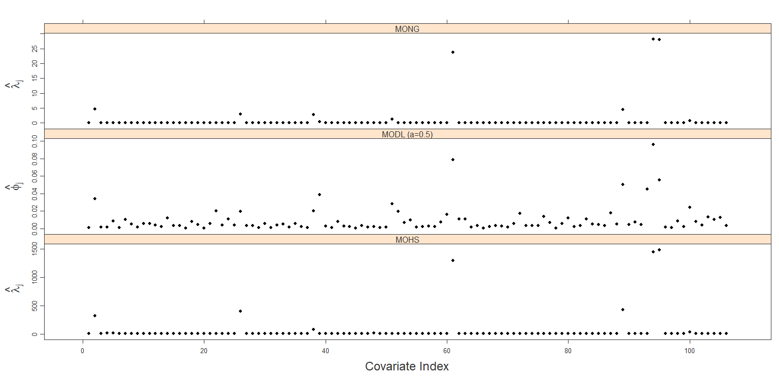 Figure 1
| Models | MSPE | SSE | ||
|---|---|---|---|---|
| All | 0 | =0 | ||
| MONG | 1.028 | 0.097 | 0.095 | 0.002 |
| MODL | 1.029 | 0.098 | 0.089 | 0.009 |
| MODL | 1.032 | 0.125 | 0.112 | 0.013 |
| MOHS | 1.030 | 0.113 | 0.099 | 0.014 |
| Naive NG | 1.040 | 0.205 | 0.167 | 0.038 |
| Naive DL | 1.036 | 0.176 | 0.104 | 0.073 |
| Naive DL | 1.079 | 0.564 | 0.547 | 0.016 |
| Naive Horseshoe | 1.040 | 0.203 | 0.111 | 0.092 |
| No shrinkage | 1.059 | 0.416 | 0.080 | 0.337 |
| Selection prior | 1.028 | 0.134 | 0.134 | 0.000 |
| MBSP model | 1.029 | 0.104 | 0.092 | 0.012 |
| Models | MSPE | SSE | ||
|---|---|---|---|---|
| All | ||||
| MONG | 0.976 | 0.113 | 0.095 | 0.028 |
| MODL | 0.976 | 0.118 | 0.085 | 0.033 |
| MODL | 0.978 | 0.127 | 0.097 | 0.030 |
| MOHS | 0.978 | 0.132 | 0.098 | 0.034 |
| Naive NG | 0.978 | 0.131 | 0.091 | 0.040 |
| Naive DL | 0.980 | 0.158 | 0.083 | 0.075 |
| Naive DL | 0.994 | 0.283 | 0.251 | 0.032 |
| Naive Horseshoe | 0.982 | 0.177 | 0.083 | 0.094 |
| No shrinkage | 1.005 | 0.416 | 0.080 | 0.336 |
| Selection prior | 0.979 | 0.139 | 0.090 | 0.050 |
| MBSP model | 0.978 | 0.146 | 0.080 | 0.066 |
| Model | MSPE | DIC | ||
|---|---|---|---|---|
| MONG | 0.833 | 15580 | 370 | 16321 |
| MODL | 0.814 | 14077 | 1299 | 16676 |
| MOHS | 0.841 | 15683 | 318 | 16320 |
| Naive NG | 0.987 | 16594 | 148 | 16890 |
| Naive DL | 0.907 | 13990 | 1430 | 16851 |
| Naive DL | 0.872 | 15117 | 733 | 16584 |
| Naive HS | 0.864 | 14706 | 827 | 16361 |
| No shrinkage | 0.971 | 13453 | 2131 | 17716 |
| Selection prior | 0.845 | 17425 | 257 | 17940 |
Peer Reviews
No public reviews on file for this paper yet. If you reviewed it on a platform where reviews are public (OpenReview, ICLR, NeurIPS, ICML), you can paste yours below so the community can read it here.
Videos
No videos yet. Explain this paper in a talk, walkthrough, or lecture? Add one.
**Bayesian Variable Selection for Multi-Outcome Models Through Shared Shrinkage
**
Debamita Kundu, Riten Mitra, Jeremy T. Gaskins
Department of Bioinformatics and Biostatistics, University of Louisville, Louisville, KY 40202, USA
Abstract
Variable selection over a potentially large set of covariates in a linear model is quite popular. In the Bayesian context, common prior choices can lead to a posterior expectation of the regression coefficients that is a sparse (or nearly sparse) vector with a few non-zero components, those covariates that are most important. This article extends the “global-local” shrinkage idea to a scenario where one wishes to model multiple response variables simultaneously. Here, we have developed a variable selection method for a -outcome model (multivariate regression) that identifies the most important covariates across all outcomes. The prior for all regression coefficients is a mean zero normal with coefficient-specific variance term that consists of a predictor-specific factor (shared local shrinkage parameter) and a model-specific factor (global shrinkage term) that differs in each model. The performance of our modeling approach is evaluated through simulation studies and a data example.
Keywords: Global-local shrinkage prior, Multi-outcome model, Multivariate regression, Shrinkage, Variable selection
1 Introduction
In the context of high-dimensional data, it is critical to correctly identify a set of variables that significantly influences the responses and play an important role in prediction. Consider a set of potential regressors and a single response variable . In order to increase the precision of statistical estimates and prediction, we often consider a model of the form
[TABLE]
where many of the are exactly zero, so that only the set of regressors impact the response .
In the Bayesian context there are numerous approaches to the problem of variable selection. Mitchell and Beauchamp, (1988) proposed the “spike and slab” approach by considering a mixture prior distribution for the regressor coefficient: a zero component (spike) and a disperse component (slab). Specifically, indicator variables were used to differentiate the important regressors from the rest. When the indicator assumes the value 0, the prior for the corresponding regressor coefficient is set to follow a Gaussian with low variance. This is the zero component (spike). Otherwise it follows a Gaussian with high variance, representing the disperse component (slab). For this setup, George and McCulloch, (1993) suggested stochastic search variable selection (SSVS) for identifying a “promising” subset. This framework was later extended to incorporate several non-conjugate and conjugate priors for prior specification (George and McCulloch,, 1997). Subsequently, a related class of variable selection priors that put positive mass at 0 are based on Reversible Jump (RJ) sampling techniques (Green and Hastie,, 2009). However, these selection methods require updating each regression coefficient conditionally on all others and tend to be computationally slow and display poor mixing when used for a large number of variables.
Hence, shrinkage priors have gained popularity recently as a computationally faster alternative. Rather than using a mixture prior that can set the coefficient exactly to zero, the shrinkage approach employs priors designed to pull small signals aggressively towards zero. Many of the commonly used shrinkage models fall within the global-local (GL) shrinkage framework defined by Polson and Scott, (2010). In the usual multiple regression setting where the regression coefficient vector is believed to be sparse, the typical GL shrinkage prior for the vector would be
[TABLE]
[TABLE]
In this model controls global shrinkage towards the origin, and are the local shrinkage parameters that allows deviation in the degree of shrinkage between predictors. The typical recommendation is that should have heavy tails to avoid over-shrinking large signals, and should have substantial mass near zero. The Normal-gamma prior (Griffin and Brown,, 2010), the Dirichlet-Laplace prior (Bhattacharya et al.,, 2015) and the horseshoe prior (Carvalho et al.,, 2010) are three popular methods in this framework. A review and comparison of various variable selection methods including the shrinkage methods can be found in O’Hara and Sillanpää, (2009).
Although much of the literature focuses on the situation of multiple regression with a single response variable , the problem of variable selection when simultaneously analyzing multiple responses (multivariate regression) is much less explored. For example, multiple outcomes measuring different aspects of a patient’s health (blood pressure, glucose, etc.) may be modeled using a potentially large set of risk factor predictors. In many cases, each outcome is analyzed separately with variable selection performed unique to each outcome, but this will be inefficient if each model has the same or similar set of relevant predictors. However, borrowing strength across regression coefficients can boost the power of detecting true signals, especially if the responses share similar predictors and there is reason to believe that they exert similar influences on the responses. The gain in performance can be substantial for low to moderate sample sizes and complex noise structures. Instead of applying variable selection separately for each outcome, Brown et al., (1998, 1999) propose two approaches based on finding a common set of predictors for all models by extending the George and McCulloch,’s selection model (1993; 1997). However, by requiring predictors to affect either all outcomes or none of them, their models are often overly restrictive. Hence, in this work we focus on developing a more flexible variable selection method that encourages the inclusion of similar sets of predictors in each of the models by extending the GL shrinkage framework. Recently, Bai and Ghosh, (2018) independently explored a similar setup and proposed their Mutlivariate Bayesian Model with Shrinkage Priors (MBSP). We will discuss differences that distinguish our work in later sections. In a frequentist setting, Turlach et al., (2005) proposed a LASSO-based approach with penalties based on the maximum absolute coefficient across all outcomes for each predictor.
The layout of this manuscript is as follows. In section 2, we describe a general strategy for GL shrinkage in multivariate regression. and explore details when paired with the 3 common GL models, Normal-gamma, Dirichlet-Laplace, and horseshoe, as well as relevant posterior consistency results. Section 3 discusses posterior sampling for each of these models, and Section 4 considers simulation studies to explore the performance of our model. In Section 5 we analyze a real data set based on the yeast cell cycle data (Chun and Keleş,, 2010), and we conclude with a brief discussion in Section 6.
2 Multi-outcome Regression Coefficient Shrinkage Model
2.1 General Strategy
Consider a multi-outcome (multivariate) model with outcomes/responses, covariates and independent observations. We write the multivariate regression model in the following form,
[TABLE]
where , the row of the matrix , consists of the responses for the th observation and is the row of the model matrix which contains the predictor variables for this observation. The matrix of regression coefficients is believed to be sparse. Further, as each row of corresponds to the regression coefficients of predictor on each of the responses, we expect similar sparsity across the row. is the residual matrix. Under the normality assumption, each row of the residual matrix follows a distribution independently. For simplicity, we ignore the intercept terms for right now. Note also that throughout we assume that the columns of and have been standardized. This gives a multivariate normal distribution for the vector of responses for patient , .
Variable selection is induced through the choice of prior on the matrix. Our approach is to extend the global-local shrinkage framework to jointly model multiple responses. The general idea of our method is to share information about the importance of a covariate across all response models through a local-shrinkage parameter and use a response-specific global shrinkage parameter to allow for different scalings of the regression coefficients in the different response models. Following the usual GL framework, our prior for the coefficient matrix comes from the following general hierarchy,
[TABLE]
The choices of the local distribution and the global distribution can be borrowed from any of the common global-local models. In particular, we focus on the utility of this approach under the following three choices: the Normal-gamma prior (Griffin and Brown,, 2010), the horseshoe prior (Carvalho et al.,, 2010), and the Dirichlet-Laplace prior (Bhattacharya et al.,, 2015). The value of the local parameter will encourage similar levels of shrinkage/sparsity for all coefficients of the predictor. Following the usual GL shrinkage rules, we choose the local distribution to have heavy tails and to have substantial mass near zero (Polson and Scott,, 2010). A large allows coefficients far from zero, whereas a small will ensure all coefficients for predictor are aggresively shrunk toward zero. Note that if there is only a single response , then our approach is exactly equivalent to the usual global-local framework. Finally, note that the general framework specifies the distributions and for the global and local parameters on the scales of the standard deviation of . In some cases, it may be more natural for and/or to represent the distribution for the variance contributions and , respectively.
Despite similarities of our framework to that of Bai and Ghosh, (2018), there are several key differences between our approaches. First, their MBSP model specifies a common value for the global parameters across all models. Further, this parameter is a priori fixed based on asymptotic arguments. Conversely, we recognize that there may be variability in the global scale of the coefficients between response models, and we allows differing which are estimated from the data. Secondly, MBSP specifies the column covariance of to be proportional to , the residual covariance matrix. This choice facilitates additional conjugacy in their sampler, but we opt to allow the columns of to be independent (given the s) as a more intuitive choice. As will be shown in Section 3, we are able to retain a high degree of conjugacy and develop an efficient posterior sampler.
Having defined our general approach, we now focus on three versions of our methodology by using common shrinkage models.
2.2 Multi-outcome Normal-gamma Model
First, we apply the Normal-gamma shrinkage prior from Griffin and Brown, (2010) to our method. We refer this model as the Multi-outcome Normal-gamma Model . This yields the following hierarchy:
[TABLE]
In , comes from a distribution such that the prior mean is 1 and variance is . Hence, small values of will induce greater variability within the s and more shrinkage. The tail of thickens with increasing . A common special case involves setting which provides the Bayesian LASSO (Park and Casella,, 2008). For the prior distribution of , we consider a half-Cauchy distribution with density . The intuition behind considering half-Cauchy prior for global shrinkage parameter is its non-zero density near the origin with thick tails in the extremes. We recommend setting the scale parameter of this half-Cauchy to to provide a reasonably dispersed distribution for the s, and this choice has performed well in empirical studies. For the hyper-parameter we consider an exponential density with mean 2 to encourage slightly thicker tails in than the Bayesian LASSO.
2.3 Multi-outcome Horseshoe Model
The horseshoe prior is one of the most appealing and commonly used shrinkage priors in the literature. It became popular due to its infinitely tall spike in the density near the origin that shrinks almost everything towards zero and its flat, Cauchy-like tails that allow some parameters to escape from shrinkage. The conventional horseshoe prior places half-Cauchy priors on both the local and global contributions to the standard deviation. The Multi-outcome Horseshoe Model is defined by the following hierarchy:
[TABLE]
In its usual form, the model is not conjugate, making implementation in a standard Gibbs sampling scheme difficult and time-consuming. However, Makalic and Schmidt, (2016) proposed an efficient, conditionally conjugate sampling algorithm for fast updating by introducing data augmentation variables from an inverse gamma distribution. Since the marginal distribution of from the hierarchy and is , we equivalently write this model as
[TABLE]
Note that we define to have density function .
In both the MONG and MOHS versions, we may use the parameters to judge the importance of a predictor across all responses. The larger the local parameter the less shrinkage in the regression coefficients and the greater the predictive power. Hence, the estimated can be used as a summary of the importance of predictor across all models. In both cases, we may compare this value relative to 1, the prior mean for in MONG and the prior median in MOHS.
2.4 Multi-outcome Dirichlet-Laplace Model
In a similar manner, we also define the Multi-outcome Dirichlet-Laplace Model . Like the previous GL methods, the DL model considers the dispersion of the coefficient to be a contribution of local and global scaling terms. However, the conditional distribution of the coefficient is Laplace (double exponential) instead of the usual normal distribution. While this may not technically fall in Polson and Scott, (2010)’s GL framework, it is clearly in the same spirit, and can be paired with our multi-outcome shrinkage framework. The proposed MODL model has the following specification
[TABLE]
where is concentration parameter of the Dirichlet distribution. In this model the local parameters sum to one, and smaller values of will lead to be dominated by a few components. Since the majority of the DE scales will be approximately zero, sparsity in the is achieved. As recommended by Bhattacharya et al., (2015), we considered or for our simulation and case study.
Similar to the HS model , we can introduce auxiliary variables to facilitate sampling. One may represent the as scale mixture of normals through with . Similar to using to evaluate predictor relevance in the MONG and MOHS models, in this MODL proposal we can compare the estimated s to their prior mean . Again, larger values indicate less shrinkage and greater predictor relevance across all outcomes.
Across all models for the regression coefficients the residual covariance matrix is given an inverse Wishart prior with degrees of freedom and the identity matrix as the prior scale matrix. This gives the prior mean for as the identity matrix. As is common, we recommend responses and predictors be centered and scaled prior to analysis.
2.5 Posterior Consistency
In this section, we present a result guaranteeing posterior consistency in our model structure. For this proof, we will assume that the residual covariance matrix is fixed and known. We first state the assumptions before proving our consistency result.
Assumptions:
- (A1)
The prior is continuous in over all of . 2. (A2)
The vector of covariates are uniformly bounded. That is, there exist such that for all . 3. (A3)
The smallest eigenvalue of the design matrix is asymptotically bounded away from zero. There exists such that , where refers to the smallest eigenvalue of the matrix .
Note that (A1) represents a much more general class of prior models than our GL shrinkage framework, although our proposal clearly falls within this assumption. Throughout, we use the Frobenius norm, . Note also that any deterministic functions of the design matrix depends on the sample size . To avoid cumbersome notation we typically suppress the dependence on and refer to it as simply .
First, we state our key theorem about posterior consistency.
Theorem 1**.**
Assume a fixed, positive definite and assumptions (A1)-(A3). Let be iid from model under the true parameter value . Then for any ,
[TABLE]
That is, the posterior distribution for almost surely collapses to the true value as .
This proof along with the associated lemmas appears in the Appendix. It builds upon Schwartz’s seminal proof (Schwartz,, 1965), in combination with results for regression models from Amewou-Atisso et al., (2003) and Choi and Schervish, (2007). The argument mainly relies on the existence of an uniformly exponentially consistent (UEC) sequence of tests and a prior positivity property. The latter in Schwartz’s original proof was simply the condition that the prior mass on all Kullback–Leibler (KL) neighborhoods of the true parameter is greater than zero. However, as we show in the Appendix, this KL framework must be modified into a multi-index version for its use in models with covariates. Both of these two conditions are derived as separate lemmas that can be combined to give posterior consistency. See the Appendix for full details.
An important feature of Theorem 1 is its flexible prior condition stated in (A1). This relaxation comes at a cost, mainly assumption (A2), which essentially bounds the entries of the design matrix. In contrast, Bai and Ghosh, (2018) assume upper and lower (asymptotic) bounds on the eigenvalues of the design matrix. However, the flexibility gained under our choice is significant, as we require no condition (except continuity) on the prior for . This is much more general than the assumptions made in the consistency theorems of Bai and Ghosh, (2018) and Armagan et al., (2013). Their choices require conditions on the prior with convoluted formulas involving and the eigenvalues of the design matrix, thus restricting the choice of prior on in ways that are not straightforward.
3 Posterior Computation
As with most modern Bayesian models, inference is performed by approximating the posterior through Markov chain Monte Carlo (MCMC) methods. We describe the necessary sampling steps for each of our three models below.
3.1 MONG Model
- (i)
Sample from , where and . Here, the prior covariance matrix of , and . Throughout, we let denote the Kronecker product. 2. (ii)
For , sample , where is the generalized inverse Gaussian distribution with density , . 3. (iii)
The posterior density of does not have a conjugate distribution. The conditional posterior sampling distribution of is given by
[TABLE]
For each , an adaptive Metropolis-Hastings (MH) step is applied to attempt an update to , based on algorithm 4 of Andrieu and Thoms, (2008) applied to . 4. (iv)
Similarly, does not have a conjugate sampling density. The conditional posterior density of is given by
[TABLE]
An adaptive MH step based on the Andrieu and Thoms, (2008) algorithm is also performed here. 5. (v)
is drawn from , where .
3.2 MOHS Model
Sampling steps for MOHS model are described below.
- (i)
Sampling distribution for is the same as in MONG step (i), except here. 2. (ii)
For , sample 3. (iii)
For , sample 4. (iv)
For , sample 5. (v)
For , sample 6. (vi)
Sample .
3.3 MODL Model
For the original DL specification, (Bhattacharya et al.,, 2015) propose a block sampler that involves marginalizations over different sets of parameters. Due to sharing s across multiple outcome models, this is no longer feasible in our MODL model , and we require (adaptive) Metropolis-Hasting to jointly sample the vector of local parameters. Sampling steps are as follows:
- (i)
First sample from . The conditional posterior distribution of is as in the case of NG prior except . 2. (ii)
For , sample (marginalizing over ) from a generalized inverse Gaussian distribution . 3. (iii)
The conditional posterior density of (marginalizing over ) is proportional to
[TABLE]
where resides in the -dimensional simplex. We have used an adaptive MH algorithm by extending algorithm 4 of Andrieu and Thoms, (2008) for sampling . We sample from distribution as described below:
- •
At the iteration, sample the proposed move by
[TABLE]
The is a positive tuning parameter that controls the dispersion of the proposal distribution. Note that this choice behaves similarly to a random walk with and . The variance of our candidate is inversely related to .
- •
Calculate the MH probability , where is the proposal distribution . With probability , we accept the proposed value , and otherwise, we retain the current .
- •
Updating the tuning parameter :
[TABLE]
where is the ideal acceptance probability and the step size is . 4. (iv)
Sample independently from . The Inverse Gaussian distribution is defined by the density function . 5. (v)
Sample .
4 Simulation Study
Here we implement simulation studies to evaluate the performance of our methodology. In addition to our MONG, MOHS, and MODL methods, we consider the following competitors:
- •
Naive Normal-gamma Model: To assess the utility of sharing the local parameters across all response variables, we consider an approach that fails to make use of this information by independently placing a NG prior on the vector of regression coefficients for each model . This naive model is unable to borrow strength across models to inform the shared level of sparsity. To that end, , where all are independent from . The rest of the model is unaffected.
- •
Naive Horseshoe Model: Similar to the naive NG model, we consider applying a horseshoe prior independently for each response. In this case, , with all independently from .
- •
Naive Dirichlet-Laplace Model: We also consider a naive version of DL prior. To that end, we let . Here, independent local shrinkage parameters are drawn for each response model : .
- •
No Shrinkage Model: As a baseline that does not favor any variable selection, we consider a basic conjugate prior model. For all , to provide minimal shrinkage towards zero.
- •
Selection Prior (Brown et al.,, 1998) Model: As noted in the introduction, this approach constrains each predictor to either be in the model of all responses or to be excluded from all.
- •
MBSP Model (Bai and Ghosh,, 2018): As previously noted, this approach is similar to our MOHS model where the global parameter is common across all responses and fixed by asymptotic arguments, rather than estimated from the data. The performance of this model is obtained using their available R package MBSP.
Data are generated from the multi-response linear regression model using a design matrix whose elements are independently drawn from a standard normal distribution. Then, rows of the response matrix are independently generated from , where if , and 1 otherwise. We consider predictors, response variables, and a sample size of . We generate 100 datasets, and for each dataset and model choice we run the MCMC chain for 90,000 iterations with a burn-in of 10,000 iterations. We measure predictive performance by computing the mean square prediction error (MSPE) using the posterior mean regression coefficients and an independently generated test data set. To assess the accuracy of the regression coefficient estimation, we consider the sum of square errors (SSE). To distinguish between error of over-shrinking relevant signals and under-shrinking non-signals, we partition this SSE into the SSE over the true non-zero s and the SSE for the s that are true zeros. These quantities are determined by the following formulas:
[TABLE]
where is the number of observations in the test dataset , and and denote respectively the response and design matrices for the test set. We consider two scenarios for choosing the true regression coefficient structure. First, we consider a simple sparse matrix (Table 1), where each covariate is either important for all responses or has no contribution to the mean of any response. Table 2 presents the results for this case.
Comparing each of our multi-outcome models to their respective naive versions, we find reduced MSPE in all cases. While the difference in MSPE between models are relatively minor, there are large improvements in the coefficient estimation. Our shared shrinkage models lead to reduction in total SSE of around when compared to the respective naive version. When looking at the two components of SSE, we see clear improvement in the estimation of the coefficients that are truly zero. That is, by sharing the local parameters across the outcome models, our model is able to better identify those coefficients that should be aggressively shrunk toward zero. Our proposed model also yields similar level of predictive performance with the selection prior approach (Brown et al.,, 1998), which is perfectly suited to this choice of .
We note that the model without shrinkage is not competitive due to its large SSE in the zero coefficients. Also the naive DL with performs poorly in estimating the non-zero coefficients. Setting provides a much stronger level of shrinkage than the case. For the naive DL model, we do see more shrinkage under than , but by sharing shrinkage information across multiple responses, our MODL model is able to find an acceptable balance in the amount of shrinkage under both choices of .
Next, we consider a situation that does not have the exact same sparse structure for each response model. There are two important considerations for such a choice. First, in light of our original motivation, we are interested in a more flexible model than those require the same subset of predictors for all responses. We wish to assess the performance of our model in such a case where there are variations in the relevant predictors across models. An alternative motivation is to understand the impact of misspecification for models that assume the exact same subset of relevant predictors across all outcomes. To that end, the new true coefficient matrix in Table 3 is created by perturbing so that the true model no longer has exact sparsity across all models. We switch three of the zero coefficients from to non-zero and also change three non-zero coefficients in to zero (as denoted in bold). This potentially represents a more realistic scenario where a small subset of predictors impact all responses, but there are some minor deviations from this general rule.
The results for this simulation settings are reported in the Table 4 and are generally similar to the previous analysis. As would be expected, the gap between the shared shrinkage and the naive approaches is somewhat narrowed, but the proposed approaches continue to show lower MSPE and lower SSE than their naive counterparts in all cases. Hence, even if there are some differences in which predictors are relevant across models, sharing shrinkage information through our common local parameter structure can continue to improve estimation. The selection prior approach and MBSP model also show similar prediction performance, although both have poorer performance in the coefficient estimation relative to our approach. Of particular note, the MBSP has fairly large SSE for the zero signals, indicating a lower level of shrinkage than our proposals. Our model estimate the global parameters from the data to adjust the amount of shrinkage, whereas MBSP fixes and is unable to correct for undershrinkage in this data.
In conclusion, our three multi-outcome models perform well in those simulation studies. Using in the MODL model may lead to overshrinking, so we typically prefer . While the differences between methods are relatively minor, MONG tends to perform best among our proposals.
5 Application
We now demonstrate our methodology with the yeast cell cycle data set (Spellman et al.,, 1998) from the spls package in R. The data was first analyzed by Chun and Keleş, (2010) and also by Bai and Ghosh, (2018). In this dataset, the response matrix contains gene expression data for genes from an factor based experiment. Each column of corresponds to mRNA levels measured at 7 minute intervals across 2 hours providing a total of responses. The covariate matrix contains the binding information for transcription factors (TFs). In molecular biology, transcription factors are a diverse family of proteins which are involved in the process of transcribing, DNA into RNA. Hence, it is of common interest to identify the most significant TFs that play an important role in gene regulations.
We applied our method to capture those TFs that affect the expression levels across all time points. We perform the analysis using our proposed MONG, MODL, and MOHS models, followed by the three naive models, the no shrinkage model, the selection model (Brown et al.,, 1998) and the MBSP model (Bai and Ghosh,, 2018). Due to over-shrinkage observed in the MODL model, we do not consider its performance here. For each case, we run a burn-in for 1000 iterations followed by another 30,000 iterations. We report the MSPE by performing cross validation on 50 data sets for each model to assess the predictive power of each method. For cross validation we randomly assign of observations to the training set to estimate , and then measured the MSPE using the remaining . We also analyze the full dataset and compute the deviance information criteria as a model comparison measure (Spiegelhalter et al.,, 2002). is calculated by , where is the deviance at the posterior expectation of the parameter values and is the effective number of parameters, and smaller s are favored. is calculated as . Table 5 shows the MSPE, the deviance at the posterior expectation of the parameter values , the effective number of parameters , and the deviance information criteria (DIC) of the yeast cycle data for each model.
The MODL choice yields the lowest prediction error among our models. Consistent with the simulation study, each of the multi-outcome approaches have smaller MSPE than their respective naive counterparts. The MONG and MOHS model also yield a lower mean square prediction error by slightly outperforming the selection prior model.
When using the competitor MBSP model, the prediction error is 0.786, scoring lowest among all approaches. It appears that for this particular data application, using a fixed value of performs slightly better than our methods which require estimating global parameters. However, as noted in the simulation study, this is not always the case, and worse performance may result. Finally, we note that the R package of MBSP model only produces model estimates and not the full set of posterior samples. So we were unable to compute DIC estimates for the MBSP model.
The DIC criteria favors the MONG and MOHS models. When considering the effective number of parameters, we see that these models estimate a much sparser regression coefficient matrix than MODL. When comparing DIC between the shared shrinkage and naive models, we again see that our proposals consistently dominate their counterparts that fail to share variable selection information between responses. The selection approach from Brown et al., (1998), which requires a common set of predictors for all models performs poorly with respect to DIC. This model places the majority of the posterior probability on models with only 2 or 3 predictors. This excessive sparsity leads to high prediction error, poor model fit, and large DIC.
Based on the results from fitting the full data set, we consider the use of the local parameters as a marker of variable importance. Figure 1 graphically displays these parameters for each of the multi-outcome models. Based on the MONG results, we would consider those covariates with as evidence of a strong effect across all response models. This criterion selects 8 important TFs: SWI5, SWI6, NDD1, ACE2, STE12, HIR1, GAT3, MBP1. The 8 predictors with the largest in the MOHS model corresponds to the same 8 TFs, indicating robustness in the predictor weights across the model variations. Consistent with its large indicating less sparsity, the MODL choice demonstrates much less separation between large and small and consequently less shrinkage/sparsity in the matrix. For this MODL case, distinguishing important predictors based on the value of the local parameters will not be effective.
6 Discussion
In this paper, we have proposed a general strategy of variable selection in the multivariate regression model by sharing common local parameters across all of the response variables. We have demonstrated our approach using the Normal-gamma, Dirichlet-Laplace and horseshoe priors. Based on the results from simulation studies and the analysis of data from an mRNA experiment, we have demonstrated the utility of our approach in comparison to alternatives. Our approaches are found to be superior in terms of both predictive performance and parameter estimation. In general, we recommend the use of the MONG version of our model as it displayed consistently strong behavior across all empirical experiments, although the MODL and MOHS also performed well.
Regarding computational comparisons between our methods, the MOHS model tends to run fastest as all of its sampling distributions are conditionally conjugate. While slightly slower, MONG has comparable computational time for a fixed number of iterations. However, the MODL model tends to be computationally slower due to the sampling of data augmentation parameters . Moreover, as noted in Section 3, the mixing in this algorithm tends to be slower due to the multivariate MH sampling of . While our adaptive step is generally effective here, further algorithmic improvements may be possible here in future research.
Appendix A Appendix
Here we provide details and the proof of the posterior consistency results from Section 2.5.
For our discussion we use the term multi-index to denote a model where the individual observations belong to a common multidimensional family but are indexed by possibly different parameters . The second subscript denotes a global parameter , which in our context is the (shared) matrix of regression coefficients. Thus, in our multivariate Gaussian regression we let be the -vector representing the mean of the responses.
Recall that the KL distance between two densities is defined as . For multi-index families, we extend the definition to have a notion KL distance for each . To that end, the KL distance between the global parameter and the true value for observation can be written as
[TABLE]
where and are parameter vectors indexing the densities for observation under parameters and . We also define as the variance analogue, i.e.,
[TABLE]
We first state our Lemma 1 which establishes a uniformly exponentially consistent (UEC) sequence of tests that will be required in the proof of Theorem 1. Here, we include the dependence on by letting and denote the response and design matrices for a sample of size .
Lemma 1**.**
For any , define . Let be the test statistic based on the critical region and . Further, assume condition (A3), and let be the largest eigenvalue of . Then, for the likelihood , we have the following:
, 2. 2.
**
Proof: Proof of this lemma follows as in Lemma 1 of Bai and Ghosh, (2018).
Next, we state and prove Lemma 2 which establishes the prior positivity condition.
Lemma 2**.**
Assume a fixed , the likelihood , (A1), and (A2). Then, for all , there exists a set with , such that for all
[TABLE]
Proof: A little algebra shows that
[TABLE]
Let , , and . Then, it follows that
[TABLE]
where . From the sub-multiplicativity of the Frobenius norm, is bounded by , which is bounded by using (A2). Clearly, . Thus, a set will clearly satisfy for all . By (A1) the continuous prior assigns positive probability to any such open neighborhood . Similar steps show that for all in , the s are bounded uniformly by a constant across all , proving convergence of .
We first introduce and sketch the proof of a more general theorem that establishes posterior consistency for a wide range of multi-index models.
Theorem 2**.**
Consider a multi-index model with global parameter and independent observations , with under the true global parameter value . Further assume the following two conditions:
There exist tests such that and that for all , . Here, and are constants not depending on the parameter of interest. 2. 2.
There exists a set with , such that for all ,
[TABLE]
Then, the posterior distribution for is consistent. That is, for any ,
[TABLE]
Proof: The proof of this theorem is a combination of arguments in Schwartz, (1965), Amewou-Atisso et al., (2003) and Choi and Schervish, (2007), and we omit the technical details. Briefly the argument is as follows. The posterior probability of interest, denoted by , can be written as a ratio of integrals of two likelihood ratios in the following way
[TABLE]
where is the -ball around and is the entire parameter space. The aim is to show converges to 0 a.s. under for all .
As shown in Schwartz, (1965), we may bound using the test statistic as
[TABLE]
where and . Following the arguments from Schwartz, (1965) (also used in Bai and Ghosh, (2018) and Armagan et al., (2013)), the first condition in Theorem 2 can be shown to imply a.s. Further, a.s., for a constant that may depend on auxiliary parameters (such as and the eigenvalues of the design matrix) but not on . Similarly, the second condition of the Theorem 2 can be shown to imply that for any constant , a.s. In combination, these imply that converges almost surely to zero under the true parameter , guaranteeing posterior consistency.
We note that the proof of this theorem has a general flavor in that it only requires a UEC sequence of tests and prior positivity. The first condition can be satisfied for several settings involving multivariate Gaussian likelihoods. The second condition is applicable to a variety of model specifications and holds simply when observations are independent but not identically distributed. Of note, condition 2 was proved in Schwartz, (1965) for single-index families and later adapted to multi-index families (Choi and Schervish,, 2007). For a proof of this, we refer the reader to the proof of part A.5 in Theorem 1 from Choi and Schervish, (2007).
Proof of Theorem 1: Results from Lemmas 1 and 2 are immediately obtained from assumptions (A1)–(A3), and these lemmas establish the two conditions required for Theorem 2. Hence, Theorem 1 is proved.
The reference list from the paper itself. Each links out to its DOI / PubMed record.
- 1Amewou-Atisso et al., (2003) Amewou-Atisso, M., Ghosal, S., Ghosh, J. K., and Ramamoorthi, R. (2003). Posterior consistency for semi-parametric regression problems. Bernoulli , 9(2):291–312.
- 2Andrieu and Thoms, (2008) Andrieu, C. and Thoms, J. (2008). A tutorial on adaptive MCMC. Statistics and Computing , 18(4):343–373.
- 3Armagan et al., (2013) Armagan, A., Dunson, D. B., Lee, J., Bajwa, W. U., and Strawn, N. (2013). Posterior consistency in linear models under shrinkage priors. Biometrika , 100(4):1011–1018.
- 4Bai and Ghosh, (2018) Bai, R. and Ghosh, M. (2018). High-dimensional multivariate posterior consistency under global–local shrinkage priors. Journal of Multivariate Analysis , 167:157–170.
- 5Bhattacharya et al., (2015) Bhattacharya, A., Pati, D., Pillai, N. S., and Dunson, D. B. (2015). Dirichlet–Laplace priors for optimal shrinkage. Journal of the American Statistical Association , 110(512):1479–1490. PMID: 27019543.
- 6Brown et al., (1999) Brown, B., Fearn, T., and Vannucci, M. (1999). The choice of variables in multivariate regression: A non-conjugate Bayesian decision theory approach. Biometrika , 86(3):635–648.
- 7Brown et al., (1998) Brown, P. J., Vannucci, M., and Fearn, T. (1998). Multivariate Bayesian variable selection and prediction. Journal of the Royal Statistical Society: Series B (Statistical Methodology) , 60(3):627–641.
- 8Carvalho et al., (2010) Carvalho, C. M., Polson, N. G., and Scott, J. G. (2010). The horseshoe estimator for sparse signals. Biometrika , 97(2):465–480.