Resurgent Extrapolation: Rebuilding a Function from Asymptotic Data. Painleve I
Ovidiu Costin, Gerald V. Dunne

TL;DR
This paper introduces a novel numerical method combining resurgent asymptotics, Borel summation, Pade approximants, and conformal mapping to accurately extrapolate functions from asymptotic data, demonstrated on Painleve I.
Contribution
It develops a general, elementary extrapolation technique that surpasses existing methods in precision, applicable to a broad class of problems including Painleve I.
Findings
High-precision extrapolation across the complex plane.
Outperforms state-of-the-art numerical integration methods.
Applicable without relying on Painleve integrability.
Abstract
Extrapolation is a generic problem in physics and mathematics: how to use asymptotic data in one parametric regime to learn about the behavior of a function in another parametric regime. For example: extending weak coupling expansions to strong coupling, or high temperature expansions to low temperature, or vice versa. Such extrapolations are particularly interesting in systems possessing dualities. Here we study numerical procedures for performing such an extrapolation, combining ideas from resurgent asymptotics with well-known techniques of Borel summation, Pade approximants and conformal mapping. We illustrate the method with the concrete example of the Painleve I equation, which has applications in many branches of physics and mathematics. Starting solely with a finite number of coefficients from asymptotic data at infinity on the positive real line, we obtain a high precision…
Click any figure to enlarge with its caption.
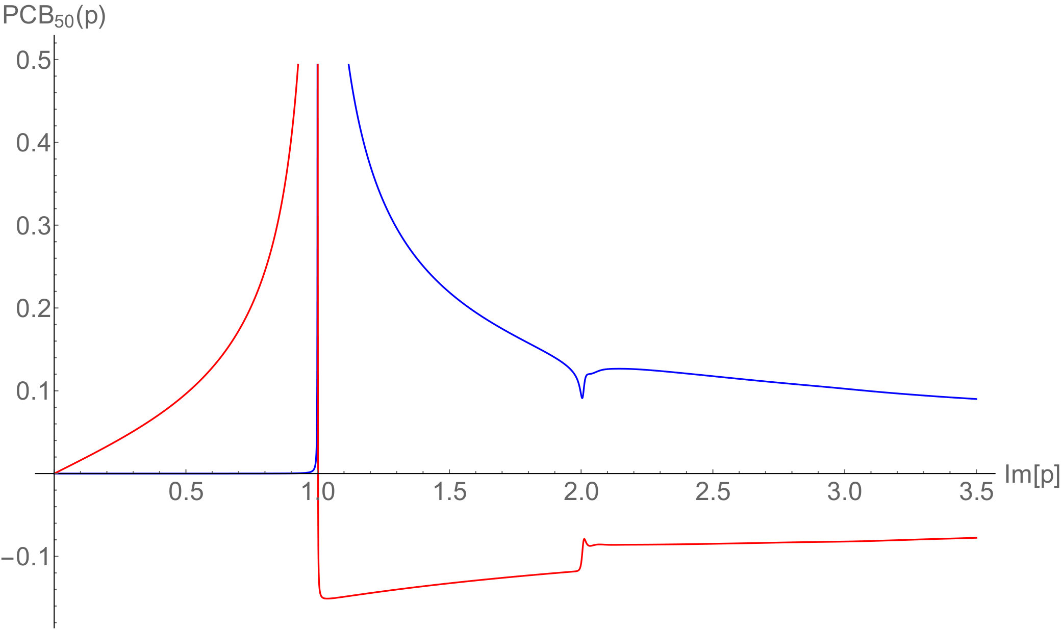 Figure 1
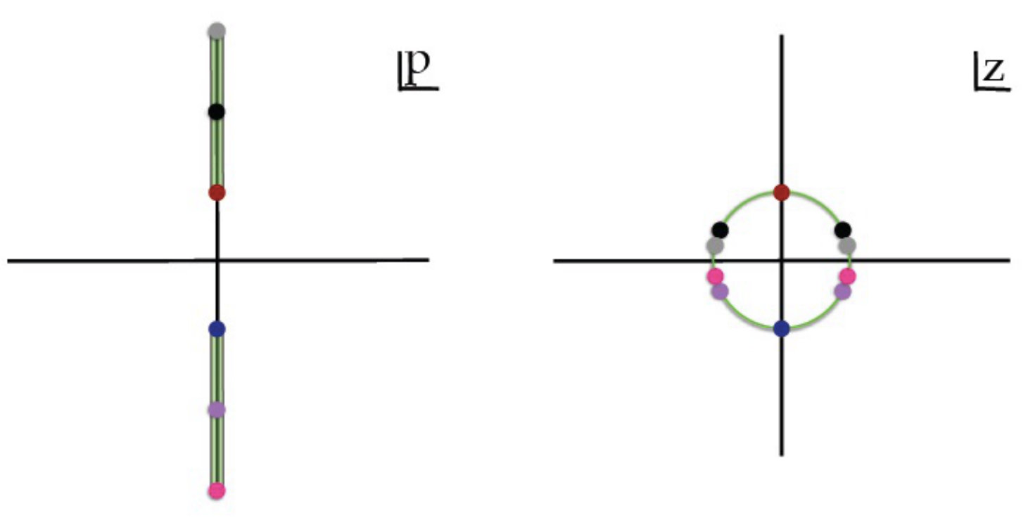 Figure 2
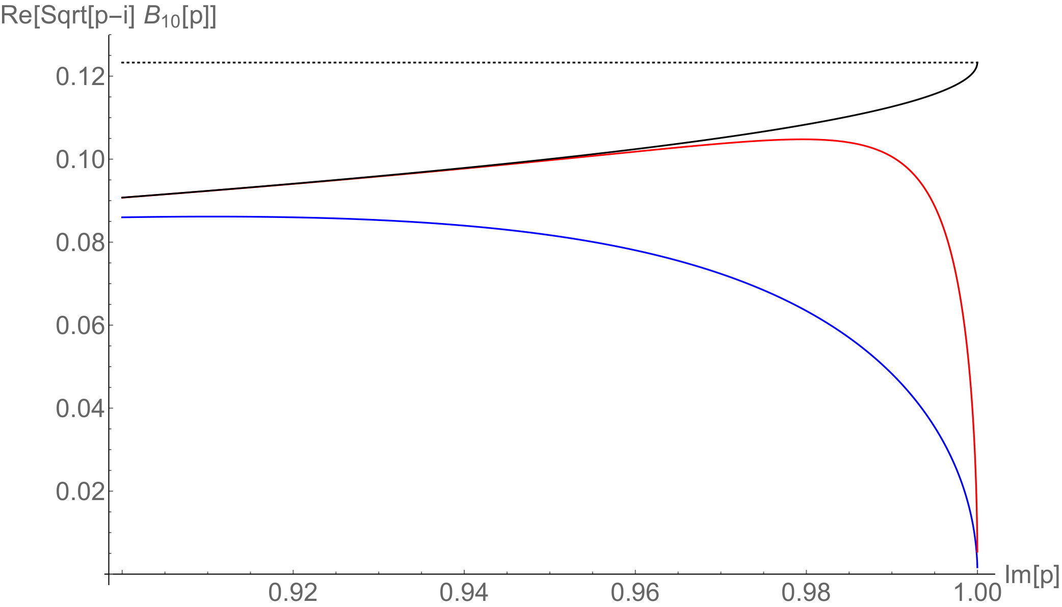 Figure 3
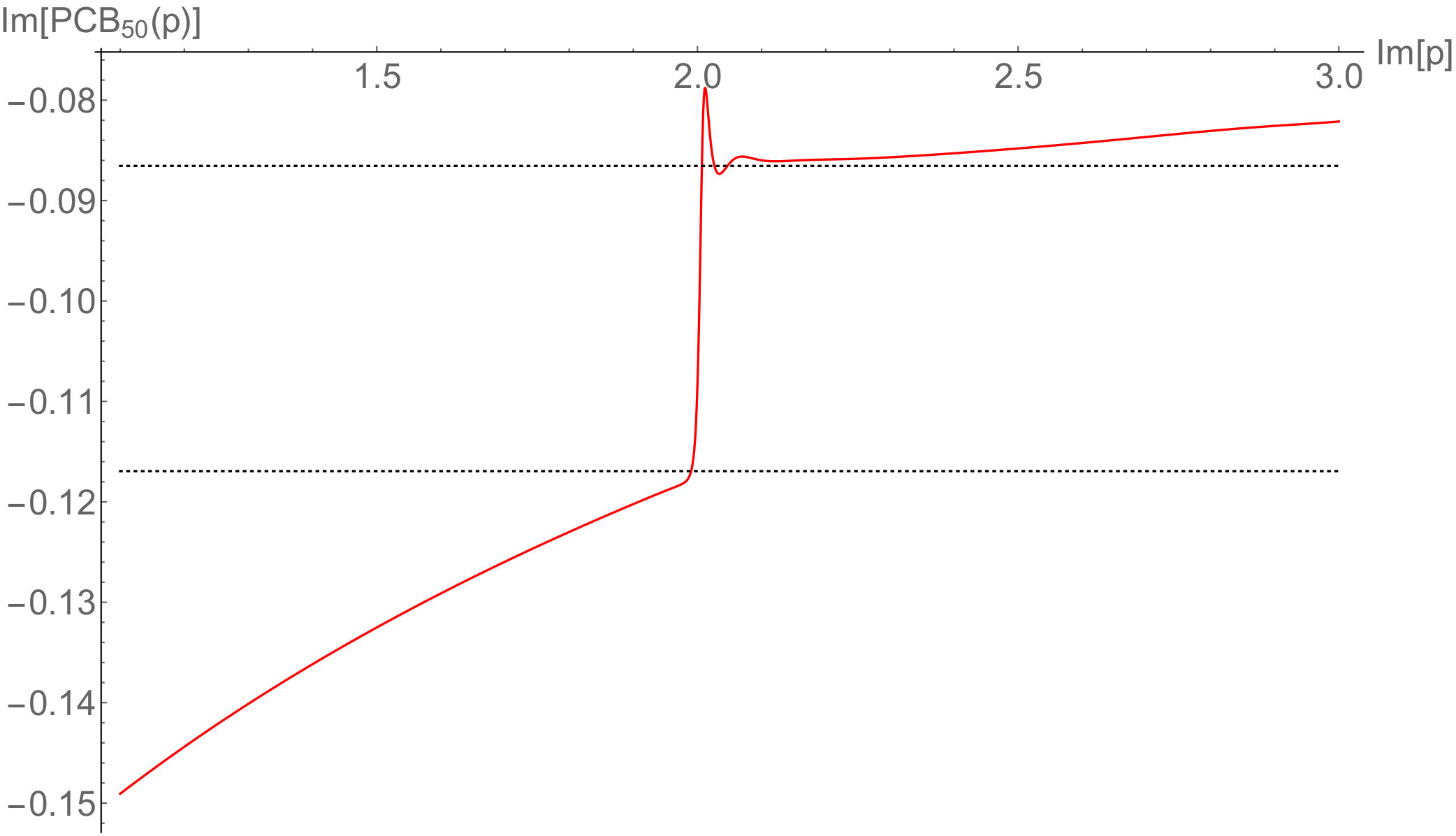 Figure 4
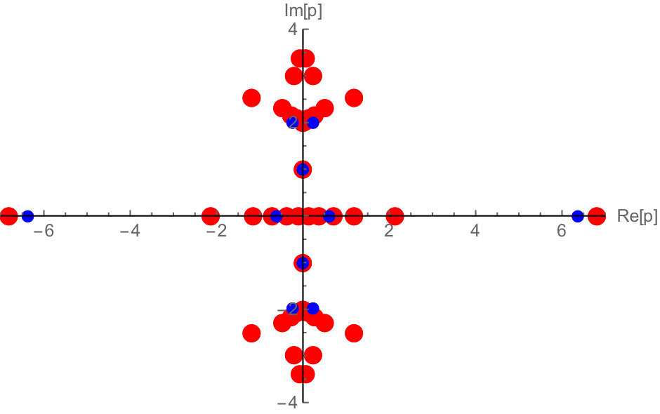 Figure 5
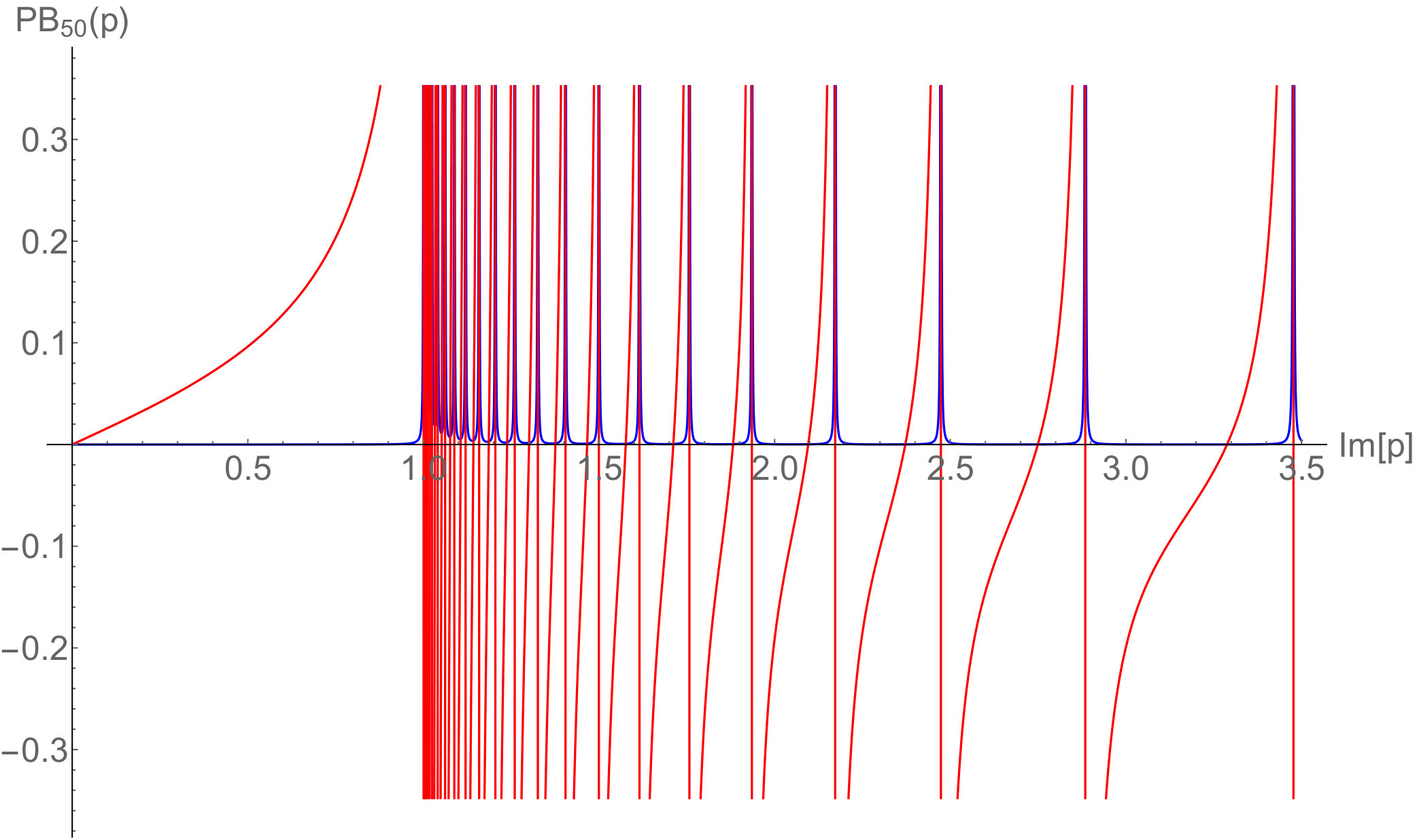 Figure 6
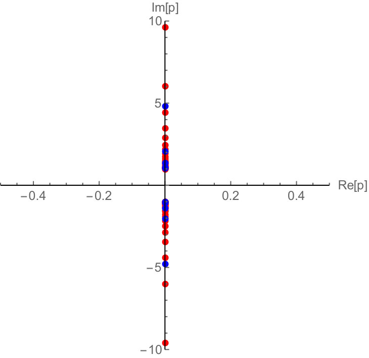 Figure 7
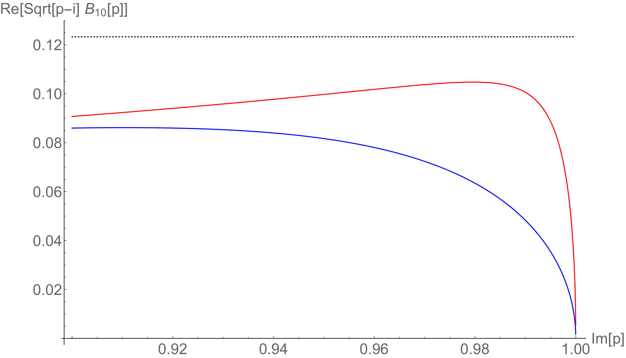 Figure 8
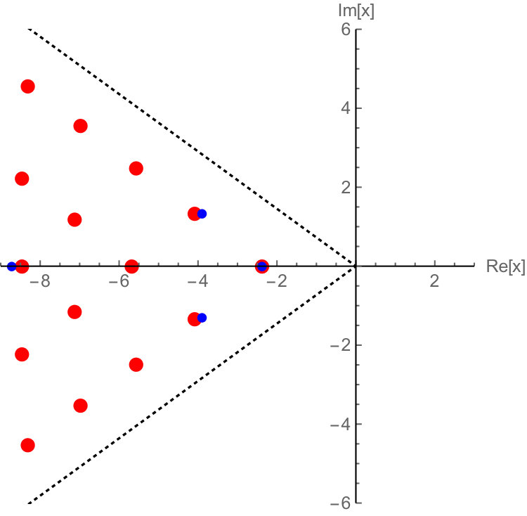 Figure 9
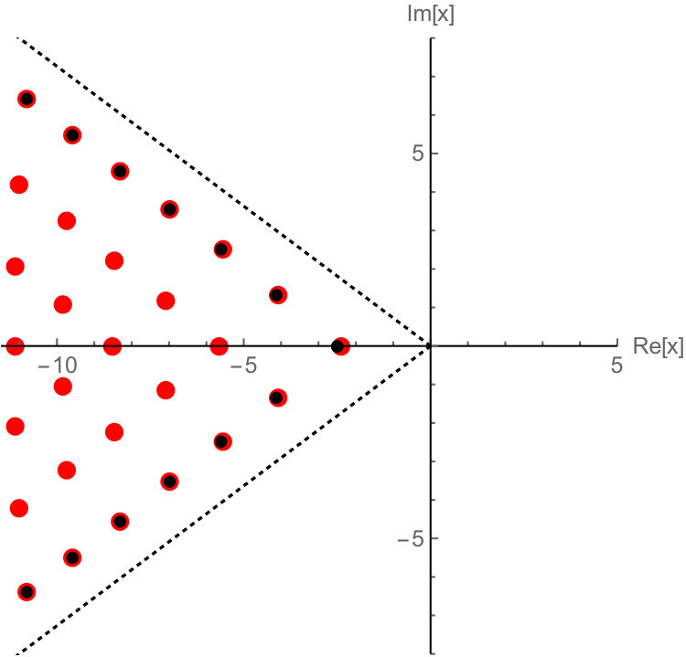 Figure 10
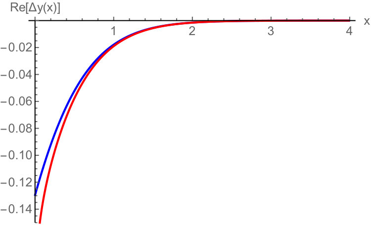 Figure 11
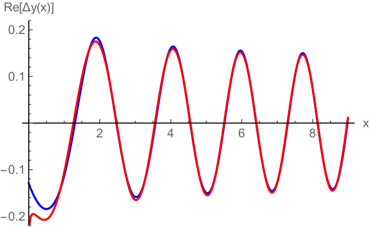 Figure 12
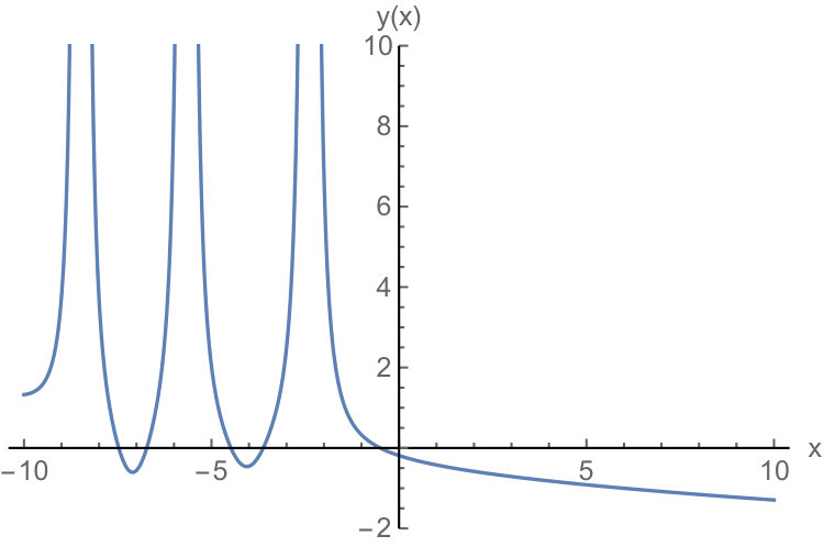 Figure 13
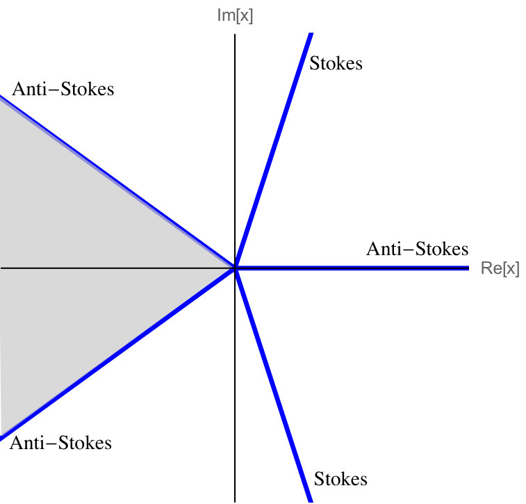 Figure 14
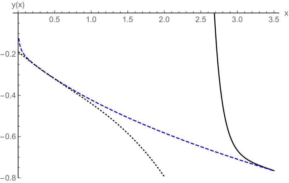 Figure 15
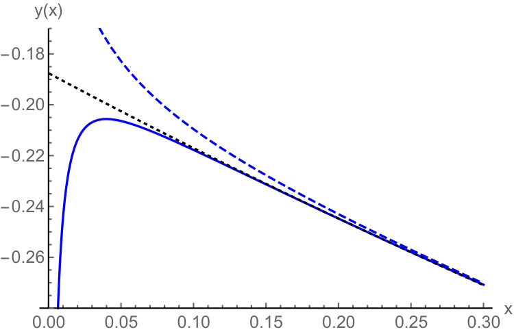 Figure 16
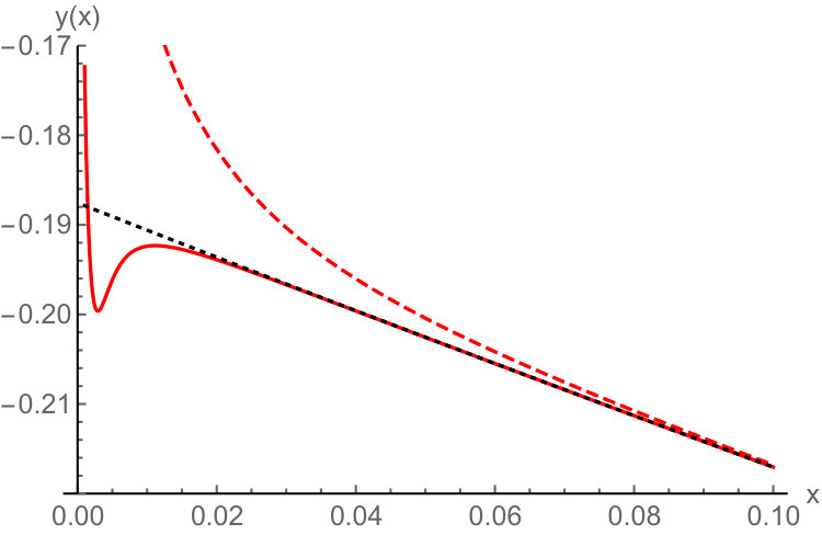 Figure 17
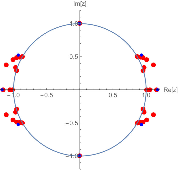 Figure 18
| pole label | pole location |
|---|---|
| 1 | -2.38416876956881663929914585244925489 |
| 2 | -4.07105552317228805393+1.33555121517567079952 i |
| 3 | -4.07105552317228805393-1.33555121517567079952 i |
| 4 | -5.57356521477+2.48916297098 i |
| 5 | -5.57356521477-2.48916297098 i |
| 6 | -5.664602914 |
| pole label | second expansion constant |
|---|---|
| 1 | -0.0621357392261776408964901416401 |
| 2 | -0.1491925267759824-0.0650559915206451 i |
| 3 | -0.1491925267759824+0.0650559915206451 i |
| 4 | -0.2485278-0.1390038 i |
| 5 | -0.2485278+0.1390038 i |
| 6 | -0.238327 |
Peer Reviews
No public reviews on file for this paper yet. If you reviewed it on a platform where reviews are public (OpenReview, ICLR, NeurIPS, ICML), you can paste yours below so the community can read it here.
Videos
No videos yet. Explain this paper in a talk, walkthrough, or lecture? Add one.
Resurgent Extrapolation: Rebuilding a Function from Asymptotic Data. Painlevé I
Ovidiu Costin1 and Gerald V. Dunne2
1 Department of Mathematics, The Ohio State University, Columbus, OH 43210
2Department of Physics, University of Connecticut, Storrs, CT 06269
Abstract
Extrapolation is a generic problem in physics and mathematics: how to use asymptotic data in one parametric regime to learn about the behavior of a function in another parametric regime. For example: extending weak coupling expansions to strong coupling, or high temperature expansions to low temperature, or vice versa. Such extrapolations are particularly interesting in systems possessing dualities. Here we study numerical procedures for performing such an extrapolation, combining ideas from resurgent asymptotics with well-known techniques of Borel summation, Padé approximants and conformal mapping. We illustrate the method with the concrete example of the Painlevé I equation, which has applications in many branches of physics and mathematics. Starting solely with a finite number of coefficients from asymptotic data at infinity on the positive real line, we obtain a high precision extrapolation of the function throughout the complex plane, even across the phase transition into the pole region. The precision far exceeds that of state-of-the-art numerical integration methods along the real axis. The methods used are both elementary and general, not relying on Painlevé integrability properties, and so are applicable to a wide class of extrapolation problems.
I Introduction
Since exact solutions are rare in physics, asymptotic analysis is a common and powerful method for studying physical systems at extreme values of the relevant parameters, such as couplings, or masses, or temperature, or density, etc. For non-trivial physical systems, it is usually only possible to generate a finite number of terms in such an expansion. This raises the important question: how much information about the function being computed is encoded in this finite set of terms, generated in one particular asymptotic region? One class of such questions is the ”central connection problem”: how can one extrapolate from strong coupling to weak coupling, or high temperature to low temperature, or high density to low density? This may enable access to the more difficult regime of intermediate values (neither small nor large) of coupling, or temperature, or density. Another class of questions involves extrapolation of the physical parameter from real values to complex values, or vice versa, a paradigm of which is the Lee-Yang-Fisher characterization of phase transitions in terms of complex zeros of the physical partition function lee-yang ; fisher-zeros . Motivated by these considerations, in this paper we study numerical methods to extrapolate finite-order perturbative expansions obtained in one parametric regime, at infinity in our chosen variable, down to zero and then throughout the entire complex plane. Extrapolation is of course a well-studied problem fisher-series ; carl-book ; zinn-qft ; kleinert ; caliceti , and our new contribution is to demonstrate how and why ideas from resurgent asymptotics dingle ; ecalle ; costin-book ; sauzin ; Aniceto:2013fka ; Dorigoni:2014hea ; gokce significantly improve the numerical reach of such extrapolations. A subsequent paper cd-2 uses resurgent asymptotics to provide precise analytic estimates of the amount of information that can be extracted from a given number of terms, also based on the precision to which these terms are known. An intuitive explanation of why resurgence provides an advantage is that resurgent functions have an orderly structure in the Borel plane, which suggests that it may be possible to characterize or parametrize a resurgent function with a relatively small number of coefficients, if the extrapolation method is able to encode the resurgent structure in an efficient way. In this sense, our motivation also includes the possibility to extend conventional numerical algorithms to incorporate resurgent structure explicitly.
In this paper, we study the extrapolation of a particular concrete example, the Painlevé I equation. This choice is made for several reasons: (i) the Painlevé non-linear differential equations have many interesting applications in physics and mathematics clarkson ; mccoy-wu ; mason ; gromak ; fokas ; forrester-book ; tracy-widom ; bonelli , with the Painlevé I equation being of particular interest for matrix models and 2d quantum gravity DiFrancesco:1993cyw ; Fokas:1990wb ; silvestrov ; david ; marino-matrix ; (ii) the Painlevé I solutions have non-trivial analytic structure in the complex plane costin-odes ; costin-dmj ; costin-costin-inventiones ; costin-costin-huang ; boutroux ; kapaev ; kitaev ; joshi ; takei ; dubrovin ; novokshenov ; Garoufalidis:2010ya ; Aniceto:2011nu ; costin-huang-tanveer ; Lisovyy:2016qig ; Iwaki:2015xnr , which illustrates extrapolation from large to small parameter, and also Stokes phase transitions in the complex plane; (iii) the known analytic structure of Painlevé solutions permits high-precision diagnostic tests of the quality of our extrapolations. We stress that even though the Painlevé equations are of course very special, since they are integrable in the sense of Painlevé ince , the methods we use do not rely on this integrability. The class of resurgent problems is much larger than that of integrable problems, and indeed resurgence applies to all “natural problems” ecalle , for example those based on differential, or difference, or integral, equations, and so resurgent extrapolation methods are expected to have broad applicability in physics.
Section II explains how to generate our input ”perturbative data” for the Painlevé I equation, and outlines the goals of our extrapolation. Section III reviews the well-known ideas of Borel summation, Padé approximants and conformal mapping applied to extrapolation along the real axis, as applied to Painlevé I. We show that conformal mapping in the Borel plane significantly improves Padé-Borel extrapolation, and in Section IV we argue that this is because the conformal mapping reveals and encodes the underlying resurgent structure of the function being computed. In Section V we introduce a re-expansion method, based on Padé analysis in the physical plane, using our high-precision extrapolation along the real axis, which yields an extrapolation throughout the complex plane, crossing the phase transition into the tritronqueé pole region. Remarkably, only a modest amount of starting ”perturbative data” is required in order to obtain non-trivial information about this phase transition and the structure of the pole region, which we confirm by comparing with known connection formulae and asymptotic estimates of pole locations.
II Painlevé I Equation: “Perturbative” Asymptotic Input Data
The Painlevé I equation (referred to below as PI) in standard form reads nist-painleve ; joshi ; dubrovin :
[TABLE]
Seeking a smooth real solution at large positive leads to an asymptotic expansion of the form
[TABLE]
where , and with this choice of normalization all the expansion coefficients are rational numbers [see (7)]. We define the natural ”Écalle time” variable
[TABLE]
It is convenient to extract the overall square root behavior and define the function by
[TABLE]
In terms of the PI equation (1) becomes:
[TABLE]
where the overdot symbol denotes . The asymptotic expansion (2) for becomes a asymptotic expansion for :
[TABLE]
where the are the same numerical coefficients as in (2). Our strategy will be to analyze the function , and then use it to reconstruct the physical PI solution via the definitions (3)-(4).
The rational expansion coefficients in (2) and (6) are generated from the recursion relation
[TABLE]
We take a certain number, , of these coefficients as our input “perturbative data”:
[TABLE]
Our goal is to learn as much as possible about the function , starting solely from the perturbative input data (8). The Painlevé I equation (1) is used in our analysis to generate the input data [i.e., the coefficients in (8)], and later as a diagnostic tool to test the level of precision of the resulting extrapolation.
We have the following specific technical goals:
Extrapolation of the formal ”perturbative” expansion at in (2), starting with a finite number of terms, along the real axis all the way down to . This is the classical central connection problem for PI, for which there is no known closed-form solution. This is an analogue of determining strong-coupling behavior from weak-coupling asymptotics, or vice versa. 2. 2.
Extrapolation of the function into the complex plane, once again starting just from the formal ”perturbative” expansion at in (2), with a finite number of terms. At this stage, resurgent asymptotics begins to play a crucial role, both in terms of increased numerical precision, and also in terms of how much of the complex plane can be explored accurately. 3. 3.
As a first step of the extrapolation into the complex plane, we show that the perturbative large data in (8) permits a remarkably high-precision extraction of the PI Stokes constant, which is known analytically from isomonodromy methods fokas ; kapaev and also from resurgent asymptotics costin-costin-inventiones ; costin-costin-huang . This enables probing of Stokes transitions, and access to higher Riemann sheets, purely from the asymptotic data on the positive real line. This is an analogue of determining non-perturbative effects from perturbative data. 4. 4.
Exploration of the transition into the PI pole region. It is well known that while the general solution to PI has poles throughout the complex plane, distributed asymptotically according to those of an associated Weierstrass elliptic function boutroux ; kapaev ; kitaev ; joshi , the formal expansion (2) defines Boutroux’s tritronquée solution to PI, which has poles in the complex plane only in a wedge region of opening angle centered on the negative real axis dubrovin ; costin-huang-tanveer . We seek to explore this pole region numerically, mapping out its distribution and properties, once again starting just from the formal ”perturbative” expansion at in (2), with a finite number of input coefficients. This is an analogue of probing a phase transition using perturbative expansion data generated from a point well away from the transition region. The behavior of the PI function changes radically as one crosses into the pole region, and its asymptotic trans-series expansion undergoes a dramatic rearrangement: the formal expansion (2) is completely different from the form of the function in the pole region: see Eq. (34). We seek to learn as much as possible about this transition from the finite perturbative input data in (8).
In our numerical extrapolation procedure we combine and compare several standard methods, such as Borel summation, Padé approximants and conformal mapping fisher-series ; carl-book ; zinn-qft ; kleinert ; caliceti . We incorporate ideas from resurgent asymptotics, with the goal of developing new extrapolation methods of increased precision and enlarged region of validity. Resurgence explains why conformal mapping is such a powerful step in this analysis. The resurgence of the Painlevé I equation is well established by general theorems and explicit computations Garoufalidis:2010ya ; Aniceto:2011nu ; costin-huang-tanveer ; costin-costin-inventiones ; costin-costin-huang ; marino-matrix ; costin-odes ; costin-dmj ; Iwaki:2015xnr , and here our numerical analysis provides further numerical evidence of these features.
III Extrapolation Along the Real Axis
In this Section we extrapolate the PI solution , starting with a finite number of terms in its formal asymptotic expansion (2) at , along the positive real axis down to , using various combinations of standard techniques, combined with some new improvements motivated by resurgent asymptotics. We compare the increased level of precision as the extrapolation method is refined. We perform our extrapolation directly on the formal asymptotic expansion (6) of the function defined in (4), and then map back to the physical PI solution using the definitions (2)–(4).
III.1 Borel Transform
The first observation is that the perturbative coefficients in (2) and (6), generated from the recursion formula (7), alternate in sign and grow factorially fast in magnitude. The alternating sign property is directly correlated with the choice of overall sign in (2) kapaev ; joshi ; novokshenov . With just 10 perturbative coefficients , straightforward Richardson extrapolation carl-book identifies the leading rate of growth as
[TABLE]
with the overall coefficient correct to 4 digits. Using 50 input coefficients permits a high-precision numerical identification of the overall coefficient, as well as extraction of subleading corrections:
[TABLE]
One can verify that the coefficients of the subleading corrections coincide with the low order coefficients of the expansion about the first exponential term in the trans-series expansion of the solution, as implied by general results of resurgent asymptotics dingle ; ecalle ; berry-howls ; sauzin ; costin-book ; Aniceto:2013fka ; Dorigoni:2014hea ; gokce .
The factorial growth in (9)-(10) implies that the expansions (2) and (6) are formal divergent series, and therefore a natural next step is to define the Borel transform carl-book ; costin-book as the inverse Laplace transform of :
[TABLE]
The formal series for in (6) is recovered by the Laplace transform:
[TABLE]
Thus, the task of extrapolating and analytically continuing the function [and therefore also the Painlevé solution ] along the real axis, and into the complex plane, becomes the problem of understanding the singularity structure and analytic continuation of the Borel transform in the complex -plane, the Borel plane. The pragmatic question is:
How much can we learn about the Borel function from just a finite number of perturbative coefficients of the small expansion defined in (11)?
III.2 Padé Analysis of the Borel Transform
The Borel transform series (11) has a finite radius of convergence, equal to 1, in the Borel plane. This follows from the large-order growth in (9), and can also be seen from a simple ratio test fisher-series . It is also encoded in the distribution of poles of a Padé approximation to the Borel transform: see Fig. 1, which indicates singularities at . Given coefficients in a truncated Borel transform
[TABLE]
and noting that it is a polynomial of degree , we form the off-diagonal Padé approximant graffi-simon ; baker ; pade ; carl-book
[TABLE]
where and are polynomials of degree and , respectively. This Padé approximant step is completely algorithmic, and is indeed a built-in function in Mathematica and Maple. The Padé-Borel poles are shown in Fig. 1, for , and for . These poles are interlaced by the associated Padé zeros. Padé approximants represent a branch cut by a string of interlaced poles and zeros, so the Padé-Borel transform suggests the existence of branch cuts along the imaginary axes, with branch points at .
As a side-comment, we note that we have found that it is more numerically stable, especially when dealing with larger values of , to convert the Padé approximant to its partial fraction decomposition:
[TABLE]
where the sum is over the Padé poles , the zeros of , with associated residues .
Since the Padé approximant is a rational function of , the partial fraction expression in (15) is in principle equivalent to the Padé expression in (14), but the increased numerical stability of (15) arises because the Padé expression at large order tends to have very large coefficients in both numerator and denominator, thereby causing instabilities due to massive cancellations. In contrast, the residues and poles in the partial fraction expression (15) are much smaller in magnitude, and so the evaluation is more stable. This is a typical instability of Padé approximants. The resulting improved numerical stability of the partial fraction form can be important for subsequent numerical integrations over , such as the Laplace transform integral in (12), required for returning to the original functions and in the physical and planes.
The Padé-Borel approximant in (14)-(15) is simple to compute, and it provides a significant extrapolation down the positive real line of the asymptotic expansion (2) of the PI solution . This is illustrated in Fig. 2, in which we plot the extrapolation obtained starting with terms. As a diagnostic comparison, we also plot [black dotted curve] the first four terms of the Taylor expansion of at the origin, using the initial conditions at the origin for the PI tritronquée solution joshi : . Fig. 2 strongly suggests that the Padé-Borel extrapolation approaches the tritronquée solution as , while the ”raw” Borel extrapolation begins to diverge from this behavior at . So, just 10 terms at are required for the Padé-Borel extrapolation to extrapolate accurately down to . In the next Section we show that by combining the Padé-Borel method with conformal mapping we obtain a dramatic improvement on this already impressive precision of the Padé-Borel extrapolation.
Having determined the location of the leading singularities, the next step is to determine the nature of these singularities. There are several complementary ways to do this. A simple method is to use Darboux’s theorem, which relates the nature of singularities to the large-order growth of coefficients of expansions about some other point henrici ; guttmann . The large-order growth in (9) implies that the leading singularities at are square root singularities:
[TABLE]
for some constant . This can also be extracted from the distribution of the interlacing Padé poles and zeros, but the Darboux analysis is simpler. Furthermore, invoking resurgence, the constant in (16) is directly related to the Painlevé I Stokes constant: . In Fig. 3 we plot the approach to the leading singularities, at , of the Padé-Borel approximation (14) to the Borel function, for . Fig. 3 displays rough numerical evidence for the approach to half the known Stokes constant for PI, marked as a horizontal dotted line. The Padé-Borel transform (14) is much better near the singularity than the raw Borel transform (13), but the behavior very close to the singularity still deviates from this resurgent expectation. With more input coefficients (larger ) the curves approach closer to the Stokes value, but the deviation persists close to the singularity. This will be probed to significantly higher precision in the next Section, in which we introduce more powerful tools than just Padé-Borel. Compare, for example, with Fig. 7.
III.3 Conformal Mapping of the Borel Plane
To refine our numerical exploration of the properties of the Borel transform function , we define a conformal map from the doubly-cut Borel plane into the unit disc in the plane:
[TABLE]
See Fig. 4. This maps the cuts along the imaginary axis in the Borel plane to the unit circle in the complex plane. The leading singularity at is mapped to . The resurgent second singularity at , on either side of the cut, is mapped to . Similarly, the resurgently repeated singularities at , map to points on the unit circle at , which approach as . Thus the point at infinity in the plane maps to . Conformal mapping combined with Borel transforms is a well-known technique in physical applications kleinert ; caliceti ; thooft ; kazakov ; zinn-qft , and here we quantify its improvement over the Padé-Borel transform discussed in the previous section, and we also use resurgent asymptotics to explain why such a significant improvement occurs.
We define a Padé-Conformal-Borel transform by the following algorithmic steps:
For a given number of input coefficients, we evaluate the truncated Borel transform in (13) at the conformally mapped location, :
[TABLE]
By construction, this function is analytic inside the unit disc in the -plane. 2. 2.
Re-expand about to the same order as the original Borel transform in [i.e., to ], and then construct a Padé approximant of the resulting truncated Taylor expansion, in the plane:
[TABLE] 3. 3.
Invert the conformal map, evaluating the -plane Padé approximant (19) at :
[TABLE]
These steps of conformal mapping, followed by re-expansion and Padé approximation, and inverting the conformal map, yield our global approximation (20) to the Borel transform function in the original Borel plane, which we call the “Padé-Conformal-Borel transform”. We stress that these steps are purely algorithmic, and furthermore they do not rely on any special integrability properties of the Painlevé I equation. In the next Sections we illustrate the numerical advantages of this conformal mapping procedure.
III.4 Increased Precision from the Padé-Conformal-Borel Transform
The first indication of higher precision using the Padé-Conformal-Borel transform, compared to the Padé-Borel transform, comes from performing the numerical inverse Borel transform integration in (12) to reconstruct the function , and hence the Painlevé I solution in the original plane using (3)-(4). This leads to the numerical evaluation of an extrapolation of the PI solution along the positive axis, using as input terms of its asymptotic expansion (2) at :
[TABLE]
Here we can replace the Borel transform function by either its Padé-Borel or Padé-Conformal-Borel approximation, defined in (14) or (20) respectively. Figs. 5 and 6 compare the reconstructed function using the Padé-Borel transform [dashed curves], and using the Padé-Conformal-Borel transform [solid curves], for and , respectively. For reference, the dotted black line shows the (convergent) expansion of at the origin, using the approximate tritronquée initial values joshi : and . Figs. 5 and 6 show that both Borel transforms, and , lead to remarkably precise extrapolations from down to very small values of , even though the extrapolations are based on just 10 or 50 input coefficients from the asymptotic expansion at . However, we observe that in both cases the Padé-Conformal-Borel transform leads to a higher precision extrapolation at small . In Section V we show how to obtain even better precision all the way to , and also into the negative region and the complex plane.
IV Extrapolation into the Complex Plane: Resurgence
In this Section we discuss how and why the Padé-Conformal-Borel transform in (20) provides a much more precise representation of the true Borel transform function than the Padé-Borel transform in (14). The source of this improvement is the resurgent structure underlying the original asymptotic expansion, which is encoded more precisely by the Padé-Conformal-Borel transform. While the two Borel functions and are very similar along the positive real axis, important differences arise in the complex plane, especially as one approaches the singularity lines on the imaginary axis (see, for example, Figs. 10, 11, and 12, below). This affects the precision with which the contour of the Laplace transform in (21) can be deformed, thereby restricting the region of the complex plane into which the Painlevé I function can be analytically continued with precision.
IV.1 Precision Evaluation of the Painlevé I Stokes Constant
Invoking resurgence of the PI function , the behavior of the Borel transform function near its first singularities at determines the Painlevé I Stokes constant, and therefore governs the associated exponential corrections. This can be used as a precise numerical test of resurgence. Recall from Fig. 3 that the Padé-Borel function shows hints of the expected square root singularity behavior near the first singularity, but deviates as approaches very close to . After conformal mapping, the Padé-Conformal-Borel transform is dramatically more precise in the vicinity of these first singularities, even with just input coefficients, as shown in Fig. 7. In fact, starting with just coefficients, the behavior of the Padé-Conformal-Borel transform near the leading singularity determines the Stokes constant to 4 digits of precision. And with digits we obtain 23 digits of precision. By contrast, probing the Padé-Borel transform near its first singularities allows just 1 digit of precision, at best. This is a dramatic improvement, which translates into a significant enlargement of the region of the complex plane in the physical variable that can be accurately probed using the inverse Borel transform (21).
IV.2 Resurgent Structure of Poles of the Padé-Conformal-Borel Transform
The underlying reason for the remarkable improvement of the Padé-Conformal-Borel transform is that the conformal map reveals the resurgent structure in the Borel plane, which is hidden in the pole structure of the Padé-Borel transform shown in Fig. 1. The conformal map separates and resolves the sub-structure of the Borel singularities, showing the repetition of singularities at integer multiples of the first singularities, as expected for a resurgent solution to a non-linear differential equation such as the Painlevé I equation (1) ecalle ; costin-dmj ; costin-book ; costin-odes ; costin-costin-inventiones ; Aniceto:2013fka ; Dorigoni:2014hea ; sauzin ; gokce .
To see this, consider the poles in the conformally mapped plane of the Padé-Conformal-Borel function defined in (19). These are shown in Fig. 8, for and . These poles display the resurgent structure of the problem. The poles at are the conformal map images of the leading square root branch points at in the Borel plane. Significantly, the conformal map has converted these branch cut singularities to simple poles, with residue proportional to the PI Stokes constant. Furthermore, these leading poles have been separated from the other singularities. This separation of the singularities according to their resurgent structure is a key factor in the improved precision of the subsequent numerical evaluations. Further observations concerning the plane poles of the Padé-Conformal-Borel function are:
There are no poles inside the unit disc in the plane, since for any the function is analytic inside the unit disc, by construction111In general, Padé may produce spurious poles, for example with anomalously small residues; these can be filtered if necessary trefethen , but we did not encounter this situation in this problem.. The poles appear on or outside the boundary of the unit disc. 2. 2.
The poles on the boundary of the unit disc in the plane are the conformal map images of plane singularities on the cuts along the imaginary axis. 3. 3.
The leading square-root singularities at have been conformally mapped to simple poles at , whose residue determines the Stokes constant with remarkable precision. (Note that if the leading singularity were not of square root form, the conformal map would not map it to a pole; however, mapping to a pole can be achieved by suitable re-definition and convolution transformations. See the discussion in the Conclusions.) 4. 4.
The poles accumulating at are the conformal map images of singularities accumulating (from either side of the cuts) at in the plane. We also see an indication of poles accumulating at , which are the conformal map images of singularities at in the plane. With higher values of , further plane singularities at higher integer multiples of are resolved. 5. 5.
The poles outside the unit disc in the plane correspond to information about the Borel transform on higher Riemann sheets, arising from analytic continuation across the plane cuts. This information can be used for further numerical refinement.
This resurgent structure of singularities can also be seen in the Borel plane. Fig. 9 shows the separation of the Borel singularities in the plane after conformal mapping. Fig. 9 displays the inverse conformal maps of the plane poles in Fig. 8. With terms [red dots] we see clearly the accumulation of singularities at , in addition to an indication of singularities at . It is straightforward to generate more perturbative input coefficients (i.e. larger ), to reveal even higher singularities. Contrast this with Fig. 1, showing the poles of the Padé-Borel transform, before the conformal map, which shows no resurgent structure of repeated singularities.
This is not just a qualitative indication of the higher-order resurgent structure: the conformally mapped Borel transform also encodes quantitative information about the resurgent singularities. For example, comparing Figs. 3 and 7, we see that the coefficient of the leading singularity can be resolved by the Padé-Conformal-Borel function , but not by the Padé-Borel function . Turning to the higher resurgent singularities, at integer multiplies of , we contrast the behavior along the edge of the plane cut shown in Fig. 10 [for the Padé-Conformal-Borel function ] with that shown in Fig. 11 [for the Padé-Borel function ]. The Padé-Conformal-Borel function resolves the first two singularities (with a hint of the third when zoomed-in), while the Padé-Borel function does not resolve any of the higher resurgent singularities. Fig. 12 shows a close-up of the imaginary part of the Padé-Conformal-Borel function along the imaginary axis, in which we see clearly the resurgent jump at . Furthermore, the magnitude of this jump coincides with that of the expected logarithmic behavior222The singularity is logarithmic because it is the inverse Laplace transform of the term costin-odes ; costin-dmj . at the second singularity:
[TABLE]
V Extrapolation into the Physical Complex Plane: The Origin and the Pole Region
V.1 Re-expansion Method and Precision Extrapolation to the Origin and Beyond
The fact that the Padé-Conformal-Borel transform encodes the resurgent structure of the Borel transform, even along the most difficult directions along the cuts on the imaginary axis in the Borel plane, suggests that the Laplace transform in (21) should be able to extrapolate the physical PI function throughout a much larger region of the complex plane than is possible with the Padé-Borel transform. In this Section we explore this complex extrapolation, first all the way down to , then onto the negative real axis, and then into the full complex plane. While this can be achieved by numerical contour integration, a much simpler and significantly more accurate method is the following two-step procedure.
Use the Padé-Conformal-Borel method to extrapolate from the asymptotic expansion (2) down to some small value on the positive real axis, at which point the PI equation is satisfied to very high precision. As an illustration, we choose . We extrapolate the function from along the real axis down to , and evaluate and by straightforward numerical Borel integration:
[TABLE]
Using the relation (4) between and , this yields extremely precise values for both and . This precision is quantified below. 2. 2.
Generate a Padé approximant of the PI solution in the physical plane, expanded about . This Padé approximant can be generated using the PI equation, expressing all higher derivatives in terms of and , in much the same way as the original perturbative coefficients were generated by expanding about . This step is algorithmic, but requires as input extremely precise values values of and . But this is exactly what our first step of Padé-Conformal-Borel extrapolation has produced.
To quantify the precision of the first step, we measure how well the extrapolated function satisfies the PI equation. Analogous to (23)–(24), we compute as a numerical integral, , which yields a value for . The precision at is then measured by the degree to which the PI equation (1) is satisfied. For example, using the Padé-Conformal-Borel transform to extrapolate down to , starting with just terms of the asymptotic expansion at , we satisfy the PI equation at to 12 decimal places, and with terms it is satisfied to decimal places. Had we used instead the Padé-Borel transform function , we still obtain impressive precision: 10 decimal places for , and 22 decimal places for :
[TABLE]
The precision increases as , in agreement with analytic estimates cd-2 .
This space Padé approximation provides a simple analytic continuation of into the complex plane. For example, we can evaluate directly at the origin. We thereby obtain very precise values for the tritronquée initial conditions at the origin. With terms and Padé-Conformal-Borel input we obtain
[TABLE]
and the PI equation is satisfied to 8 digit precision at the origin. With terms and Padé-Conformal-Borel input we obtain
[TABLE]
and the PI equation is satisfied to 64 digit precision at the origin. Padé-Borel input also leads to precise values at the origin, but with lower precision. This level of precision should be compared with roughly 14 digits of precision for and obtained for Painlevé equations by the best current boundary-value, initial-value and Fredholm determinant numerical methods that operate along the positive real axis fornberg ; bornemann . The ultimate reason for the remarkable improvement in precision is that our extrapolation method incorporates the resurgent structure of the function, which encodes global information about the function throughout the entire complex plane, not just along the positive real axis.
As a further application, we can further continue the reconstructed function along the negative real axis, where the PI tritronquée solution is known to have poles. Fig. 13 shows in this region, with input coefficients, with the first three (double) poles clearly visible. Even with input coefficients we accurately resolve the first pole on the negative axis. The extrapolated function goes directly across the phase transition into this pole region, which we explore in further detail in the next section.
V.2 Stokes Transition: Mapping the Tritronquée Pole Region
In this Section we cross the Stokes transitions in the physical variable, at , and map the tritronquée complex pole region. The Dubrovin conjecture dubrovin states that for the tritronquée solution to PI, which has the asymptotic expansion (2) at joshi ; kitaev ; kapaev , the only poles lie in the wedge region: . This conjecture has been proved in costin-huang-tanveer , and has been confirmed by several numerical analyses novokshenov ; bornemann ; fornberg . Here we use our resurgent extrapolation to give another high precision confirmation of this conjecture, combined with an analysis of the fine structure of the pole region.
Fig. 14 shows the poles of our analytically continued solution , obtained by combining the Padé-Conformal-Borel extrapolation with a Padé expansion at , using just [blue dots], or [red dots], coefficients as input data. We stress that given the input coefficients from (8), the rest of the computation is entirely algorithmic. We find it quite remarkable that with just 10 terms of the asymptotic expansion at , the first three poles in the tritronquée pole region can be seen with reasonable precision. With 50 terms, we resolve the first 21 poles with a high degree of precision. It is a simple matter to work with even higher values of , if further poles and/or higher precision are desired. See Fig. 15.
We see from Fig. 14 that the poles do indeed lie within the expected wedge, a numerical confirmation of the Dubrovin conjecture dubrovin . To probe the tritronquée poles more precisely, we compare them with the locations predicted by the trans-asymptotic analysis of costin-costin-inventiones ; costin-costin-huang . An asymptotic expression for the outer layer of poles in the tritronquée wedge is costin-costin-inventiones ; costin-costin-huang :
[TABLE]
and , where is proportional to the Stokes constant: . In Fig. 15 we compare the trans-asymptotic estimate in (31) with the numerical poles obtained from our Padé-Conformal-Borel procedure, starting with coefficients at . The agreement with the asymptotics is remarkable, even all the way down to for the pole closest to the origin. Asymptotic formulas for successive layers of lines of poles can be derived straightforwardly from recursion relations for adiabatic invariants costin-costin-inventiones ; costin-costin-huang .
We comment that in a very interesting paper novokshenov , Novokshenov has made a Padé expansion of the PI solution directly at the origin in the physical variable, which can be “tuned” to the tritronquée solution by adjusting the initial values and according to the requirement that the resulting Padé approximant has no poles outside the tritronquée pole region wedge . To ensure that no poles leak outside of this region, this requires an extremely delicate search procedure, profoundly sensitive to the initial values and ; and therefore a very efficient Padé algorithm was developed in novokshenov . By contrast, in our -space Padé re-expansion method (see Sec. V.1), the initial values and are automatically fixed by our high-precision Padé-Conformal-Borel extrapolation, and no search is needed at all.
V.3 Stokes Wedges and Tritronquée Connection Formulas
In this Section we plot our extrapolated PI solution , from Sec. V.1, along the Stokes and anti-Stokes lines for the tritronquée solution. These are the most interesting and nontrivial directions in the complex plane, describing the transition boundaries between the five different Stokes wedges.
Recall that the PI equation is invariant under rotation of the coordinate by , and the function by boutroux ; kapaev ; kitaev ; dubrovin ; novokshenov ; Garoufalidis:2010ya ; joshi ; takei , and the asymptotics (2) of the tritronquée solution defines the set of Stokes and anti-Stokes lines, with , as shown in Fig. 16. Our perturbative input (8), from which we have developed our extrapolation of the PI solution throughout the complex plane, was obtained from the large asymptotics along one particular direction: the anti-Stokes line along the positive real axis. The behavior of along the other Stokes and anti-Stokes lines is very different. As a precise diagnostic check of the quality of our extrapolation into the complex plane, we can test the known analytic connection formulas of the PI tritronquée solution, which relate the rotated tritronquée solutions along the Stokes and anti-Stokes lines boutroux ; kapaev ; kitaev ; Garoufalidis:2010ya .
For example, the tritronquée solution along the positive axis, and along the anti-Stokes line , at the edge of the pole region, are related by the following exact connection formula, exhibiting oscillatory behavior with a coefficient depending on the Stokes constant kapaev ; kitaev ; Garoufalidis:2010ya :
[TABLE]
Fig. 17 shows this combination using our extrapolated function , displaying the oscillatory behavior of (32), capturing accurately both the period and the amplitude. On the other hand, the tritronquée solution along the Stokes lines are related by the following exact connection formula, exhibiting exponentially decaying behavior, also with a coefficient depending on the Stokes constant kapaev ; kitaev ; Garoufalidis:2010ya :
[TABLE]
Fig. 18 shows this combination using our extrapolated function , displaying the correct exponentially decaying behavior of (33).
V.4 Fine Structure of the Tritronquée Poles
The general PI solution is known to be meromorphic throughout the complex plane boutroux ; gromak ; fokas , and to have poles throughout the complex plane, in all five Stokes wedges. Indeed, in the vicinity of a moveable pole, the general PI solution has a Laurent expansion of the following form
[TABLE]
All further coefficients of this Laurent expansion are expressed as polynomials in the two parameters and . Thus, any PI solution is completely determined by two constants, and , in the vicinity of any one of its poles. The tritronquée is special in the sense that it has poles only in one Stokes wedge dubrovin ; costin-huang-tanveer (see Sec. V.2). Since our re-expansion method produces the most precise values for the pole closest to the origin, it is natural to use this first pole, and its associated expansion constant , to characterize the tritronquée solution to PI. In fact, since there is nothing special about for the PI equation, the data is a much more natural way to characterize the tritronquée solution than giving and at the origin. High precision values for the first pole and the associated expansion constant are:
[TABLE]
These agree with previously quoted values joshi , although those values were given to significantly lower precision.
To quantify the precision of the tritronquée values in (35), we expand our extrapolated Padé function about its pole closest to the origin, , and compare the terms of the expansion with the known general form (34):
[TABLE]
We observe that the coefficient of the leading pole term equals 1 to 36 decimal places, and the next two terms vanish to 34 and 33 decimal places. The quadratic term coefficient agrees with to 31 decimal places, and the coefficient of the term equals to 31 decimal places. Furthermore, the coefficient of the term vanishes to 30 decimal places. Thus we estimate the precision of the constant as the coefficient of the term to 30 decimal places. As a further check, we note that the coefficients of the next two terms in the expansion agree with their exact values, and , to 29 and 28 decimal places, respectively.
In Tables I and II we record our results for the first 6 poles, , and the associated expansion constants, , obtained from our numerical extrapolation, based on input coefficients. The number of digits shown for each pole is determined by the method described above for , applied to each pole . The precision degrades quickly for the poles further from the origin, but this can be improved by taking larger , and also by combining with trans-asymptotic estimates such as (31), which become much more precise for the poles further from the origin. In this paper we have not implemented these refinements, but we quote these initial values because of their relevance to the quantum mechanical spectral problem for cubic oscillators, and because only very low order values exist in the literature for the first two real poles, and masoero . A more detailed numerical study of the tritronquée pole values is left for future work. This is motivated by results connecting poles of PI solutions to spectral properties of cubic oscillators masoero ; bender ; novokshenov2 , in analogy to results relating pole behavior of Painlevé III solutions with the spectrum of the Mathieu equation novokshenov-mathieu ; lukyanov ; gorsky , and pole behavior of Painlevé VI solutions to spectral properties of an associated Heun equation litvinov ; gd .
VI Conclusions
We have studied the numerical extrapolation of the solution to the Painlevé I equation (1), starting from a finite number of terms in the asymptotic expansion at . Combining standard methods of Borel transforms, Padé approximants, and conformal mapping, together with aspects of resurgent asymptotics, we obtain a surprisingly precise extrapolation throughout the complex plane. Our initial asymptotic expansion (2) generates the tritronquée solution to PI, and we tested the precision of our extrapolation by comparing it with known analytic properties such as exact connection formulae and trans-asymptotic pole expressions. The extrapolated function crosses smoothly across the non-linear Stokes transitions into the pole region. Both Padé-Borel and the conformally mapped Padé-Conformal-Borel extrapolations produce high quality extrapolations, but the latter is more accurate in a larger range of the complex plane. The ultimate reason for this is that the conformal map resolves more efficiently the underlying regularity of the resurgent structure in the Borel plane. The resurgent extrapolation method is very general, not relying on the integrability of the Painlevé I equation, and should be applicable to the much broader class of resurgent problems in physics. Several extensions and refinements of the resurgent extrapolation method are possible, which may become more relevant in other problems where fewer perturbative coefficients can be generated, and/or if these coefficients are generated with limited precision. We list some of these refinements here, and further details will be given in subsequent papers.
Duality Bootstrap: the expansion of as maps directly to the behavior of the Borel transform, and correspondingly the behavior of as maps directly to the behavior of the Borel transform. In certain cases the problem may be one of interpolation, in which some knowledge about both and is known, but one wants to interpolate between these two expansions in a way that accurately describes intermediate values of . In this case, the duality between large and small , and small and large can be used to develop an iterative ”bootstrap” procedure. In the case of PI, our extrapolation method already produced sufficient numerical precision, but in other problems this duality bootstrap can be a powerful additional tool.
Singularity Tuning: as mentioned in Sec. IV.2, the leading Borel singularity for PI is of square root character [see (16)], and is mapped to a pole by the conformal map (17). In other problems, where the leading singularity is not a square-root branch point, one can apply ramified re-definitions of the expansion parameter and Borel variable in order to engineer a leading pole after conformal mapping. This facilitates the resurgent separation of the singularities, resulting in improved precision.
Higher Riemann sheets: we observed numerically that the Padé-Conformal-Borel produces singularities on higher Riemann sheets. These singularities could be used for further higher precision tests of resurgence, and also for a systematic numerical investigation of Écalle’s medianization ecalle ; sauzin .
Continued Fractions, Orthogonal Polynomials and Padé Approximants: there is a deep connection between Padé, continued fractions, orthogonal polynomials and conformal mapping, which we discuss in detail in cd-2 , but we comment briefly on the basic ideas here. The outcome of this connection is that one can derive analytic estimates of the precision that can be obtained by Padé-Borel and Padé-Conformal-Borel with input coefficients. Resurgence appears in these extrapolations due to the fact that given terms of an expansion, Padé can predict the next term with exponential precision. Analytic continued fractions wall , in one of the most useful normalizations, are rational functions of the form
[TABLE]
where are monomials, . Given a power series, the constants and are uniquely determined by requiring that the Maclaurin series of coincides with the given series to the highest possible order allowed by the total degree of . It follows that is in fact a way of rewriting a near-diagonal Padé approximant , deg()deg(). This is an important representation of Padé approximants for a number of reasons, including the fact that the are much smaller than the Padé coefficients, and that the often have asymptotic expansions at large , which give analytic information about the series. For Painlevé I we calculated , and observed empirically that, for large , . A straightforward induction argument shows that the polynomials and satisfy two-step recurrence relations wall , which can therefore be associated with orthogonal polynomials. Then the asymptotics of follows from Szegö asymptotics of orthogonal polynomials szego . We can then estimate the successive error as , for some independent of , where the conformally mapped variable from (17) arises from solving the asymptotic recursion formulas. A deep result of Damanik and Simon characterizes the asymptotics , with small enough damanik . This can be used to show that the accuracy in of a Padé-Borel approximant with terms is , roughly the same as that of the conformally mapped Taylor series in the unit disk. In particular, if and , then ; and thus standard Padé-Borel approximants diverge everywhere on the cuts. On the other hand, for small , meaning that, well inside the unit disk, Padé-Borel gives an accuracy improvement over the Taylor series. And, away from the cuts, for large and , a standard Borel-Padé approximation has accuracy , which translates to accuracy in the physical domain . And the improvement of the conformally mapped Padé-Conformal-Borel transform in (20) over the Padé-Borel transform in (14) also scales like . Further details and applications will appear in cd-2 .
Resurgent Numerical Analysis: our results suggest that it may also be fruitful to incorporate some ideas of resurgence into the sophisticated numerical analysis methods of bornemann ; fornberg .
This material is based upon work supported by the U.S. Department of Energy, Office of Science, Office of High Energy Physics under Award Number DE-SC0010339 (GD), and by the National Science Foundation under Award Number DMS 1515755 (OC). Both authors thank the KITP at Santa Barbara for its hospitality during the Fall 2017 program “Resurgent Asymptotics in Physics and Mathematics” where much of this work was begun. Research at KITP is supported by the National Science Foundation under Grant No. NSF PHY-1125915. We thank A. Its, P. Nevai, and C. Bender for helpful discussions, comments and correspondence.
The reference list from the paper itself. Each links out to its DOI / PubMed record.
- 1(1) C. N. Yang and T. D. Lee, “Statistical theory of equations of state and phase transitions. 1. Theory of condensation,” Phys. Rev. 87 , 404 (1952); T. D. Lee and C. N. Yang, “Statistical theory of equations of state and phase transitions. 2. Lattice gas and Ising model,” Phys. Rev. 87 , 410 (1952).
- 2(2) M. E. Fisher, “The Nature of Critical Points”, pp. 1-159 in Lectures in Theoretical Physics , Vol. VII C, (Univ. of Colorado Press, 1965); M. E. Fisher, “Yang-Lee Edge Singularity and phi 3 Field Theory,” Phys. Rev. Lett. 40 , 1610 (1978).
- 3(3) M. E. Fisher, “The theory of equilibrium critical phenomena”, Rep. Prog. Phys. 30 , 615 (1967).
- 4(4) C. M. Bender and S. A. Orszag, Advanced Mathematical Methods for Scientists and Engineers: Asymptotic Methods and Perturbation Theory , (Springer, 1999).
- 5(5) J. Zinn-Justin, Quantum field theory and critical phenomena , Int. Ser. Monogr. Phys. 113 , 1 (2002).
- 6(6) H. Kleinert and V. Schulte-Frohlinde, Critical properties of phi 4-theories , (World Scientific, 2001).
- 7(7) E. Caliceti, M. Meyer-Hermann, P. Ribeca, A. Surzhykov and U. D. Jentschura, “From useful algorithms for slowly convergent series to physical predictions based on divergent perturbative expansions,” Phys. Rept. 446 , 1 (2007), ar Xiv:0707.1596 .
- 8(8) R. B. Dingle, Asymptotic expansions: their derivation and interpretation , (Academic Press, 1973).